


Abstract
A novel method is presented for predicting the common secondary structures and alignment of two homologous RNA sequences by sampling the ‘structural alignment’ space, i.e. the joint space of their alignments and common secondary structures. The structural alignment space is sampled according to a pseudo-Boltzmann distribution based on a pseudo-free energy change that combines base pairing probabilities from a thermodynamic model and alignment probabilities from a hidden Markov model. By virtue of the implicit comparative analysis between the two sequences, the method offers an improvement over single sequence sampling of the Boltzmann ensemble. A cluster analysis shows that the samples obtained from joint sampling of the structural alignment space cluster more closely than samples generated by the single sequence method. On average, the representative (centroid) structure and alignment of the most populated cluster in the sample of structures and alignments generated by joint sampling are more accurate than single sequence sampling and alignment based on sequence alone, respectively. The ‘best’ centroid structure that is closest to the known structure among all the centroids is, on average, more accurate than structure predictions of other methods. Additionally, cluster analysis identifies, on average, a few clusters, whose centroids can be presented as alternative candidates. The source code for the proposed method can be downloaded at http://rna.urmc.rochester.edu.
INTRODUCTION
With the recent discovery of new classes of functional RNA sequences, there is an increased need for tools to predict and analyze RNA structure and function (1). Often a first step in understanding the mechanism of action of an RNA is the determination of secondary structure, i.e. the set of canonical base pairs in the structure. When a large number of homologous sequences are available, comparative analysis, where the structure common to all sequences is determined, is an accurate method for predicting structure (2,3). Alternatively, with only one available sequence, the structure can be predicted either by free energy minimization using the set of stabilities fit to experiments (4–6) or with probabilistic methods using the set of sequences with known structure (7–9). For cases where there is a small set of sequences, but too few for comparative analysis, a set of algorithms have been developed to predict a secondary structure by combining comparative analysis with either free energy minimization (10–12) or probabilistic analysis (13,14).
The first widely used programs for predicting secondary structures by free energy minimization found the lowest free energy structure (15), a single best guess for the structure and a set of low free energy structures to serve as alternative hypotheses for the structure (16,17). It was then shown that all structures within a small free energy increment above the lowest free energy structure could be generated (18). The number of low free energy structures increases exponentially with both the length of the sequence and with the free energy increment, making it infeasible to study the folding ensemble by generating low free energy structures. Subsequently, Ding and Lawrence presented a method (19) for stochastic sampling from the ensemble, where the probability of sampling a structure is the probability of finding that structure in the Boltzmann ensemble. Using stochastic sampling, a relatively small number of sampled structures could be used to generate an understanding of the ensemble folding behavior.
A useful method for understanding the folding space of RNA molecules is to organize the structures into distinct classes and to compute representatives for the set of most likely classes. This methodology is powerful because of the following reason. Even though the complete folding ensemble is large, ∼1.8N structures for an RNA sequence of length N (20), a relatively small selection of the most likely distinct classes represents the statistics of features commonly found in the ensemble and provide useful alternate hypotheses for the secondary structure class. The classes of secondary structures may be defined a priori, an approach that is typified by RNAshapes (21–23), or they may be determined a posteriori by clustering predicted structures, an approach exemplified by the stochastic sampling method developed by Ding and Lawrence (19).
The performance of methods in the either of these categories can potentially be improved by utilizing multiple homologous sequences for the determination of the structure classes. Within the RNAshapes framework, this is accomplished by RNAcast (22,23), which computes the abstract shapes (21) of multiple RNA sequences within a specified energy threshold of the minimum free energy for each sequence and then finds the optimal consensus shape that is common to all the sequences. The structures for each sequence are predicted as the representative structure, referred to as ‘shrep’, of the consensus shape for each sequence. For the stochastic sampling methodology, on the other hand, extensions of the technique to multiple sequences have received limited attention. Although a heuristic iterative sampling methodology has been proposed in RNA Sampler (24), a true stochastic sampling framework has not been previously developed due to the difficulty in computing the corresponding partition function for the multiple homolog scenario.
In this article, a novel method for stochastic sampling of the space of the structural alignments of two homologous RNA sequences for the purpose of predicting common secondary structures and alignment for the two sequences is described and benchmarked. The structural alignment space is the joint space of common secondary structures and sequence alignments of the RNA sequences and the method is therefore called ‘joint sampling’. This work is enabled by and uses the previously reported PARTS algorithm (25), which developed a formal mathematical characterization of the structural alignment space of two sequences (25,26) and provided an algorithm for calculating the partition function over this space of structural alignments. Because stochastic sampling is accomplished here from a rigorous partition function, common structures and alignments are sampled according to their probability of occurring in the ensemble of structural alignments. The joint sampling method described here provides more accurate structure prediction compared with both single sequence sampling (27) and with multiple sequence methods, RNAcast (23) and RNA Sampler (24). Joint sampling also offers advantages for the alignment of sequences. The alignments obtained via joint sampling can be grouped into clusters and centroids of these clusters can provide estimates of the alignment. This methodology has the advantage that it accounts for the conserved secondary structure in estimating the sequence alignment as compared with alternatives based on sequence data alone. Results obtained with the proposed method support this hypothesis. Alignment cluster centroids provide a more accurate estimate of the alignment than a sequence alignment hidden Markov model.
The joint sampling algorithm is presented in the Methods section. The performance of the joint sampling is compared with other methods in terms of structure and alignment prediction accuracy in the Results section. Finally, a discussion of the advantages of joint sampling over single sequence sampling and the limitations of joint sampling is presented in the Discussion section.
METHODS
Figure 1 shows the steps for prediction of common secondary structures and alignment of two RNA sequences utilizing the joint sampling of the structural alignment space. First, a sample of structural alignments of the sequences is obtained via the joint sampling method. The set of structures and alignments in the sample of structural alignments are then clustered individually. The common structures and the alignment of the two sequences are predicted as the centroids of the corresponding clusters identified in the clustering process. This section describes the joint sampling method and the method employed for clustering of structures and alignments.
Figure 1.

Block diagram showing processing steps of samples of structures and alignments obtained from the joint sampling of structural alignment space.
A structural alignment 𝒮 of two RNA sequences x1 and x2 of lengths N1 and N2 refers to a joint representation of common secondary structures and the alignment of the sequences. Given 𝒮all, the set of all structural alignments between the sequences and a probability distribution P(𝒮) over the space of structural alignments, joint sampling seeks to determine a representative sample of structural alignments according to the distribution P(𝒮).
Structural alignment space and partition function
This work uses the space 𝒮all of structural alignments and the corresponding pseudo-Boltzmann distribution that is considered in the PARTS algorithm (25). The corresponding formal definition of a structural alignment can be found in (25,26). The key idea is illustrated in Figure 2, which shows an example structural alignment between two tRNA sequences RD0260 from ‘phage T5 virus’ and RD0500 from Haloferax volcanii (28). Each of the colors in Figure 2 indicates a corresponding matched helical region (25) between the two structures and the corresponding regions in the secondary structures and the alignment. The commonality of the secondary structures is ensured by requiring that all base pairs in the structures are included in the matched helical regions, which is equivalent to the requirement that the fifth-level abstract RNA shapes are identical (21) for the two structures. The probability of a structural alignment 𝒮 as defined by the pseudo-Boltzmann distribution of structural alignments (25):
| 1 |
where ΔG(𝒮) denotes the pseudo-free energy change of the structural alignment 𝒮. The ΔG(𝒮) combines scores for the common structures S1 and S2 for x1 and x2, respectively, and for alignment A in the structural alignment 𝒮. The commonality of structures is ensured by the fact that structural alignments are built with matched helical regions, which were rigorously defined previously (25). Specifically, in this work the pseudo-free energy change is computed as (25):
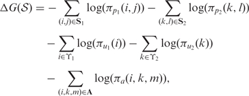 |
2 |
where S1 and S2 represent the sets of base pairs in the first and second sequences, respectively. ϒ1 and ϒ2 correspond to the sets of unpaired bases in structures of respective sequences. The πpq(r, s) is precomputed base pairing probability of nucleotides at indices r and s in sequence q, and πuq(r) is the precomputed unpairing probability of nucleotide at index r in sequence q. A denotes an alignment between the two sequences and πa(i, k, m) is the precomputed probability of alignment state m at alignment position (i, k). The m denotes an alignment state taking one of three values depending, respectively, on whether i and k are aligned, i is an insertion in sequence 1, or k is an insertion in sequence 2.
Figure 2.

Structural alignment of RD0260 and RD0500. Colored rectangles indicate the nucleotides in matched helical regions (25). (a) Common secondary structures. (b) Sequence alignment.
Efficient sampling of pseudo-Boltzmann distribution
Explicit enumeration of P(𝒮) over all possible structural alignments is computationally infeasible because the number of possible structural alignments is large even for pairs of relatively short sequences, e.g. tRNAs. Efficient sampling of the distribution P(𝒮) can be achieved via an iterative sampling algorithm, which builds a structural alignment from basic building blocks termed ‘structural alignment atoms’ (SAAs). The SAAs represent the irreducible elements of structural alignments. The decomposition of a structural alignment into SAAs is illustrated in Figure 3, which is described next in the context of joint sampling.
Figure 3.

Decomposition of a structural alignment of two hypothetical sequences into SAAs. (a) The structures of sequences x1 and x2. The bold lines represent the base pairing between nucleotides at corresponding indices. (b) The sequence alignment A between sequences. The aligned nucleotides are denoted by lines with double-headed arrows. A bold line in a sequence represents an insertion at the corresponding index in the other sequence. The dashed rectangles illustrate decomposition of the structural alignment into eight SAAs that are denoted by χn(i, j, k, l), n = 1, … , 8, such that each dashed rectangle encloses the nucleotide indices whose pairing and alignment are defined by the respective SAA. For the SAA χ3(2, 9, 3, 9), the internal and external SAAs are illustrated in (a) by the arrows on left and in (b) by grouping of corresponding SAAs.
A structural alignment 𝒮 can be decomposed into a set of SAAs {χ(i, j, k, l)}, where i and j denote nucleotide indices in x1 with i ≤ j, k and l denote nucleotide indices in x2 with k ≤ l. For each SAA χ(i, j, k, l), in the alignment A in 𝒮, the nucleotide indices (i − 1) and j of x1, are co-incident respectively, with nucleotide indices (k − 1) and l of x2. Two nucleotide positions (one from each of the two sequences) are said to be co-incident if they are either aligned, or if one nucleotide position (from one of the sequences) occurs in an insertion in that sequence that begins at a nucleotide position aligned with the second nucleotide position (from the other sequence) (10). The χ(i, j, k, l) represents one of following 11 possibilities of pairing and alignment of nucleotides at indices i, j, k and l:
Insertion of paired nucleotides at i and j.
Insertion of paired nucleotides at k and l.
Alignment of paired nucleotides at i and j to paired nucleotides at k and l, respectively.
Alignment of paired nucleotides at i and j to unpaired nucleotides at k and l, respectively.
Alignment of unpaired nucleotides at i and j to paired nucleotides at k and l, respectively.
Alignment of an unpaired nucleotide at i to an unpaired nucleotide at k.
Alignment of an unpaired nucleotide at j to an unpaired nucleotide at l.
Insertion of an unpaired nucleotide at i.
Insertion of an unpaired nucleotide at j.
Insertion of an unpaired nucleotide at k.
Insertion of an unpaired nucleotide at l.
The SAAs represent all the possible base pairing and sequence alignment interactions between co-incident nucleotides in a structural alignment of two sequences.
The requirement for four indices to specify an SAA stems from the fact that the decomposition of a structural alignment utilizing SAAs involves tracking two pairs of co-incident subsequence indices that progress from outside to inside in a manner similar to the Cocke–Younger–Kasami algorithm for stochastic context-free grammars (SCFGs) (29). In addition, the boundary conditions for co-incidence are handled appropriately in the decomposition. For example, when considering χ(i, j, k, l) for i = 1 and k = 1, the sequence indices i − 1 = 0 and k − 1 = 0 are assumed to be co-incident.
The iterative joint sampling algorithm builds a structural alignment progressively by probabilistically generating the current SAA, χ(i, j, k, l), according to the conditional distribution of SAAs in the pseudo-Boltzmann ensemble. The conditioning is predicated on the previously generated SAAs, 𝒮ext(i, j, k, l), which are referred to as the set of ‘external’ SAAs. Thus the process first generates the external-most SAA in the structural alignment, χ(1, N1, 1, N2), and subsequently generates the ‘internal’ SAAs. Given an SAA χ(i, j, k, l), the internal SAAs correspond to χ(i′, j′, k′, l′) such that i ≤ i′ < j′ ≤ j, k ≤ k′ < l′ ≤ l and external SAAs correspond to χ(i′, j′, k′, l′) such that i′ ≤ i, j ≤ j′, k′ ≤ k, l ≤ l′. The conditional probabilities, P(χ(i, j, k, l)|𝒮ext(i, j, k, l)), are obtained with the PARTS partition function calculation, which provides the necessary normalization of the probabilities. The partition function is obtained efficiently via dynamic programming and careful attention is paid in order to ensure that each structural alignment is considered once and only once. The normalizations are accessible in the arrays calculated by the PARTS algorithm, described previously (25). Details of the actual implementation are available in the Supplementary Material included with the article.
Figure 3 illustrates a decomposition of a structural alignment of two hypothetical sequences into SAAs. The dashed rectangles in Figure 3 illustrate the external to internal decomposition of the structural alignment into eight SAAs such that each dashed rectangle encloses the nucleotide indices whose pairing and alignment are defined by the respective SAA. The pairing and alignment of nucleotides as defined by each of eight SAAs is indicated below in the order, which they would be generated by the iterative sampling algorithm.
χ1(1, 10, 1, 11): paired nucleotides at 1 and 10 in x1 are aligned to unpaired nucleotides at 1 and 11 in x2, respectively.
χ2(2, 9, 2, 10): paired nucleotides at 2 and 10 in x2 are both inserted.
χ3(2, 9, 3, 9): paired nucleotides at 2 and 9 in x1 are aligned to paired nucleotides at 3 and 9 in x2, respectively
χ4(3, 8, 4, 8): paired nucleotides at 3 and 8 in x1 are aligned to paired nucleotides at 4 and 8 in x2, respectively
χ5(4, 8, 5, 8): unpaired nucleotide at 4 in x1 is aligned to unpaired nucleotide at 5 in x2.
χ6(5, 8, 6, 8): unpaired nucleotide at 5 in x1 is aligned to unpaired nucleotide at 6 in x2.
χ7(6, 8, 7, 8): unpaired nucleotide at 6 in x1 is aligned to unpaired nucleotide at 7 in x2.
χ8(7, 8, 8, 8): unpaired nucleotide at 7 in x1 is inserted.
The steps of iterative sampling are listed in Algorithm 1. The algorithm begins by computing the partition function and then by generating SAA χ(1, N1, 1, N2). Every consecutive iteration for generation of an SAA involves computation of the conditional probability distribution P(χ(i, j, k, l)|𝒮ext(i, j, k, l)), followed by sampling of the distribution to obtain an SAA χ(i, j, k, l). Then the indices i, j, k, l are updated based on the SAA χ(i, j, k, l) such that the indices point to nucleotides whose pairing and alignment states are not yet established. The structures, S1 and S2, and sequence alignment A are updated according to the pairing and alignment of nucleotides as defined by χ(i, j, k, l). Lastly, χ(i, j, k, l) is added to 𝒮ext. The algorithm terminates when the pairing and alignment of all the nucleotides in both sequences are defined by the SAAs generated. The structural alignment is formed by S1, S2 and A.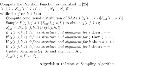
For ease of descriptions and understanding, Algorithm 1 represents the simplified scenarios of structural alignments with only singly branched structures. The generation of structural alignments with multi-branched structures proceeds similarly by replicating the sampling for each branch and accounting for branching in structures when conditional probability distribution of SAAs is sampled. The computational complexity of iterative sampling algorithm is O(N21 N22) in the general multi-branched case. The details of the iterative sampling algorithm are included in the Supplementary Material.
Clustering samples of structures and alignments
Given a sample of structural alignments generated by the iterative sampling algorithm, the sample sets of common secondary structures of each sequence and of sequence alignments are clustered individually using the ‘diana’ (30) algorithm from the R Statistical Computing Software Package (31). The ‘diana’ algorithm uses the base pair distance between structures or aligned position distance between sequence alignments while clustering a sample of structures or sequence alignments, respectively. For each sample, diana generates a ‘dendrogram’ that is used to obtain 20 different clusterings of the sample such that k-th clustering contains k-th clusters of the sample for 1 ≤ k ≤ 20. The optimal number of clusters kopt is determined as the number of clusters that maximizes ‘Calinski–Harabasz pseudo-f statistic’ (CH Index) (32). Secondary structure and alignment predictions are then obtained from the clustering corresponding to the optimal number of clusters for the sample of structures and alignments, respectively. This is the same clustering procedure used for single sequences by Ding et al. (27). The details of the computation of CH Index and cluster centroid structures are presented in the Supplementary Material.
Following the clustering, a representative structure or alignment, called the ‘cluster centroid’, is computed for each of the identified clusters using the method of Ding et al. (27). The centroid of a cluster is the structure or alignment, in the full ensemble of structures and alignments, that has the smallest average distance of base pairs or aligned positions, respectively, to all structures or alignments in the cluster. The centroid of the most populated cluster, the centroid of the sample set and the ‘best’ centroid that with the smallest distance to the known structure or alignment, serve as estimates of the structure or alignment and the accuracy of these estimates is evaluated. (Because the number of clusters is small, the best is representative of the performance when the cluster centroids are presented as alternate hypothesis for the structure or alignment). The sample of structures and alignments are also used to predict the probabilities of base pairing and alignment, which are employed as measures of confidence for the corresponding base pairing or nucleotide alignment in the centroid structures and alignments. The probabilities of base pairing and sequence alignment are estimated as the frequency of these events in the sample of structures and alignments.
Note that the distances between structures are in units of base pairs and the distances between alignments are in units of aligned positions. Because the distances in difference units are difficult to combine into a single meaningful distance between structural alignments, the samples of structures and alignments are clustered individually instead of clustering samples of structural alignments. The accuracy of structure or alignment prediction obtained through this individual clustering is also seen to be similar to that obtained by clustering structural alignments based on a naive distance function that sums up the distance in structures and alignments, despite their different units. It is worth noting that the independent clusterings of the sample of structures and the sample of alignments do not guarantee that a valid structural alignment will be produced.
Scoring predicted structures and alignments
The accuracy of predicted centroid structures and alignments are reported in terms of sensitivity and positive predictive value (PPV). The sensitivity is the fraction of known features correctly predicted. For structures, the features are base pairs and, for alignments, the features are aligned positions. The PPV is the fraction of predicted features that appear in the known structure or alignment. The number of correctly predicted base pairs is determined by counting the base pairs that match base pairs in the known structure with up to one nucleotide ‘slippage’ in one index (33,10). A base pair between nucleotides at indices i, j, therefore, is considered correctly predicted if there is a base pair in the known structure between nucleotides at indices i, j or i + 1, j or i, j + 1 or i − 1, j or i, j − 1. Average sensitivities and PPVs are the means of the sensitivities and the PPVs obtained for the individual predictions over the chosen dataset, respectively.
RESULTS
The performance of the joint sampling was compared with:
The single sequence sampling method that samples the Boltzmann Distribution of structures of an RNA sequence (19) as implemented in the RNAstructure software package (4). The default options were used to run RNAstructure single sequence sampling.
RNA Sampler (24), which is a method for predicting common structures of multiple RNA sequences based on iterative sampling of conserved helical regions in structures of all sequences. RNA Sampler was used with default options.
RNAcast (22), which computes all the consensus shapes for multiple RNA sequences. RNAcast is used to compute all the consensus shreps (21) (shape representatives) with energies at most 40% above the energy of minimum free energy structures of the sequences (command line option ‘-c 40’). A 40% threshold was used because the method could not find consensus shapes for some of the sequences with threshold values <40%.
The maximum a posteriori (MAP) structure prediction by the PARTS algorithm (25).
The alignment prediction accuracy of joint sampling is compared with a sequence alignment hidden Markov model (10), and MAP alignment prediction from the PARTS algorithm. All methods are evaluated on datasets containing 2000 randomly chosen pairs of tRNA sequences from the Sprinzl tRNA Database (28), 2000 randomly chosen 5S rRNA sequences from the 5S Ribosomal RNA Database (34) and 40 randomly chosen pairs of RNase P sequences from the RNase P Database (35). The dataset is the same dataset that was utilized in benchmarking experiments performed in a previous paper (25), so results are directly comparable with previous benchmarks on Dynalign (10), FOLDALIGN (12), StemLoc (13), Consan (14), LocARNA (36) and single sequence structure prediction based on free energy minimization (4). The cluster analysis was performed on the generated sample of structures and sequence alignments obtained by generating 1000 samples via joint sampling.
The first benchmarks test the hypothesis that the structure space is significantly reduced by joint sampling as opposed to single sequence sampling due to the implicit comparative analysis in joint sampling. The average base pair distance between structures within a cluster is plotted against the number of clusters in Figure 4. For the number of clusters, k, in the plot, the average base pair distance between structures within the same cluster is computed for k = 1–20. The resulting average base pair distance value is a measure of dissimilarity of structures within same cluster for a given number of total clusters. Figure 4 shows that the dissimilarity of structures within a cluster is significantly lower for clusters generated by joint sampling as compared with clusters obtained by the single sequence sampling.
Figure 4.

Average within cluster base pair distance for clusters of sampled structures. (a) tRNA. (b) 5S rRNA. (c) RNase P.
Table 1 shows the structure prediction accuracy of joint sampling and single sequence sampling for ensemble centroids, largest cluster centroids, the best scoring centroid; prediction accuracy of shrep of minimum rank consensus shapes and accuracy of shrep that has lowest distance to known structure, i.e. best shrep, predicted by RNAcast; and structures predicted by RNA Sampler. Consistent with what was previously observed with single sequence sampling (27), the largest cluster centroid structure is more accurate, on average, than the PARTS MAP algorithm for the 5S rRNA dataset and it is marginally more accurate for the RNase P dataset in both sensitivity and PPV. On the tRNA dataset, the joint sampling is, on average, less accurate than the PARTS MAP algorithm. The largest cluster centroids from joint sampling are, on average, more accurate than the largest centroids from single sequence sampling and the minimum rank consensus shape representative structures computed by RNAcast. The biggest cluster centroid structures predicted by joint sampling are more accurate than structures predicted by RNA Sampler for the 5S rRNA and RNase P datasets and the methods have comparable accuracy over the tRNA dataset.
Table 1.
Prediction accuracy of structures generated by joint sampling and cluster analysis; single sequence sampling and cluster analysis; structures predicted by RNAcast and RNA Sampler; and structures in minimum pseudo-free energy structural alignment computed by PARTS MAP algorithm for tRNA, 5S rRNA and RNase P datasets
| Joint sampling |
Single sampling |
RNAcast |
PARTS | |||||||||||||||||
|---|---|---|---|---|---|---|---|---|---|---|---|---|---|---|---|---|---|---|---|---|
| Biggest cluster |
Ensemble |
Best cluster |
Biggest cluster |
Ensemble |
Best cluster |
Minimum rank |
Best shrep |
RNA sampler |
MAP |
|||||||||||
| Sensitivity | PPV | Sensitivity | PPV | Sensitivity | PPV | Sensitivity | PPV | Sensitivity | PPV | Sensitivity | PPV | Sensitivity | PPV | Sensitivity | PPV | Sensitivity | PPV | Sensitivity | PPV | |
| tRNA | 0.808 | 0.862 | 0.806 | 0.866 | 0.835 | 0.895 | 0.716 | 0.683 | 0.699 | 0.716 | 0.857 | 0.874 | 0.660 | 0.631 | 0.866 | 0.844 | 0.824 | 0.849 | 0.825 | 0.874 |
| 5S rRNA | 0.737 | 0.766 | 0.736 | 0.768 | 0.754 | 0.791 | 0.642 | 0.609 | 0.619 | 0.636 | 0.748 | 0.739 | 0.693 | 0.648 | 0.786 | 0.751 | 0.664 | 0.753 | 0.690 | 0.742 |
| RNase P | 0.631 | 0.746 | 0.630 | 0.748 | 0.640 | 0.761 | 0.613 | 0.644 | 0.600 | 0.681 | 0.667 | 0.735 | N/A | N/A | N/A | N/A | 0.462 | 0.602 | 0.627 | 0.746 |
| Overall accuracy | 0.725 | 0.791 | 0.724 | 0.794 | 0.743 | 0.816 | 0.657 | 0.645 | 0.639 | 0.678 | 0.757 | 0.783 | N/A | N/A | N/A | N/A | 0.650 | 0.735 | 0.714 | 0.787 |
The joint sampling and single sequence sampling algorithms were used to generate 1000 structures of tRNA and rRNA sequences and 5000 structures for RNase P dataset. Biggest cluster, accuracy of centroid structure of biggest cluster generated by cluster analysis; Ensemble, the centroid structure of the whole sample set, Best cluster, accuracy of cluster centroid that has the smallest base pair distance to the known structure; Minimum rank, accuracy of shape representative in the minimum rank consensus shape computed by RNAcast; Best shrep, accuracy of the shrep (shape representative) that has the smallest distance to known structure among all shreps predicted by RNAcast within 40% energy interval above energy of minimum free energy for the corresponding sequence; PARTS MAP, accuracy of structures in the minimum pseudo-free energy structural alignment computed by PARTS algorithm; Overall accuracy, the average accuracy of the methods over all the datasets; N/A, cases where RNAcast required more memory than available on the system. The experiments are performed on a system with 8 GB of main memory running Fedora Core 5.
The effect of the sample size in stochastic sampling was investigated by generating 10 different samples of 1000 structures for all sequences in the tRNA dataset by the proposed joint sampling method and evaluating the variability in the average accuracy of the biggest cluster centroid structures in each sample. Over the 10 different stochastic sampling instantiations, the biggest cluster centroid had an average sensitivity of 0.808 and a standard deviation of 1.84 × 10⁻⁴. The corresponding PPV numbers were 0.862 and 1.87 × 10⁻⁴, respectively. The low standard deviations indicate that the chosen sample size is adequate and the stochastic nature of the sampling introduces the negligible variability in the reported numerical results.
The ensemble centroid structure, a representative structure for the whole sample, is marginally higher in PPV and lower in sensitivity as compared to the biggest cluster centroid structures for both joint sampling and single sequence sampling. This is an expected result because the ensemble centroid structure contains the base pairs that are found in most structures within the sample, therefore, the ensemble centroid tends to include fewer base pairs that are more likely to be correctly predicted than cluster centroids (37).
The best cluster centroid, which represents the most accurate possible prediction from among all of the identified clusters, is more accurate than MAP structure prediction of PARTS and comparable with the best cluster centroid structure of single sequence sampling for all three datasets. It is also comparable with the accuracy of the best shape representative among all the shapes computed by RNAcast on tRNA and 5S rRNA datasets. This structure, however, can only be determined by knowing the actual structure. The average number of clusters identified for each dataset is shown in Table 2 for the sampling methods (averaged over the number of clusters determined for each sequence). It can be seen that the clustering methods provide a relatively small number of clusters and therefore a small number of alternatives for predicted structures. Furthermore, the number of clusters generated by stochastic sampling is also smaller than the average number of consensus shapes computed by RNAcast, which is also included in Table 2.
Table 2.
Average number of clusters of structures identified by the cluster analysis for joint and single sequence sampling methods and number of consensus shapes computed by RNAcast over tRNA, 5S rRNA and RNase P datasets
| tRNA | 5S rRNA | RNase P | |
|---|---|---|---|
| Joint sampling | 6.86 | 4.05 | 3.21 |
| Single sampling | 4.62 | 4.04 | 2.85 |
| RNAcast | 9.15 | 78.31 | N/A |
Table 3 shows the alignment prediction accuracy for the joint sampling, for the lowest pseudo-free energy structural alignment estimate as computed by PARTS MAP algorithm (25), and the most likely alignment that is predicted by the alignment hidden Markov model. The biggest cluster centroid alignment is more accurate compared with the sequence alignment computed by the hidden Markov model and the sequence alignment predicted by PARTS. The ensemble centroid alignment has the same sensitivity as the largest cluster centroid and slightly higher PPV. The best cluster centroid is the most accurate compared with all other methods; note again that the best is chosen from a relatively small set of candidate centroids.
Table 3.
Prediction accuracies of alignments generated by joint sampling and cluster analysis, the alignments in the minimum pseudo-free energy structural alignment as predicted by PARTS MAP algorithm (denoted by ‘PARTS MAP’) and the ML sequence alignment computed by sequence alignment hidden Markov model (denoted by ‘pHMM’)
| Biggest cluster |
Ensemble |
Best cluster |
PARTS MAP |
pHMM |
||||||
|---|---|---|---|---|---|---|---|---|---|---|
| Sensitivity | PPV | Sensitivity | PPV | Sensitivity | PPV | Sensitivity | PPV | Sensitivity | PPV | |
| tRNA | 0.857 | 0.856 | 0.857 | 0.858 | 0.881 | 0.881 | 0.843 | 0.847 | 0.794 | 0.787 |
| 5S rRNA | 0.940 | 0.946 | 0.940 | 0.947 | 0.951 | 0.957 | 0.925 | 0.932 | 0.906 | 0.902 |
| RNase P | 0.744 | 0.720 | 0.744 | 0.721 | 0.753 | 0.729 | 0.743 | 0.705 | 0.743 | 0.703 |
| Overall | 0.847 | 0.841 | 0.847 | 0.842 | 0.862 | 0.856 | 0.837 | 0.828 | 0.814 | 0.797 |
The sequence families are denoted on the rows and prediction accuracy of Biggest cluster centroid, Ensemble centroid, Best cluster centroid, PARTS MAP and pHMM (pairwise hidden Markov model) are denoted on columns.
Figure 5 shows the plot of PPV versus sensitivity of base pairs whose estimated probabilities, obtained by joint sampling or the single sequence sampling, are higher than a chosen threshold. The threshold is incremented from 0.0 to 1.0 in steps of 0.001 to obtain a corresponding plot in each case. In each plot, the top-right corner corresponds to perfect prediction of base pairs, i.e. both sensitivity and PPV of 100%. The plots for joint sampling are closer to the top-right corner than plots for single sequence sampling. The sensitivity and PPV of base pairs with estimated posterior probability of base pairing greater than 0.50 is marked in Figure 5 with a diamond on each curve in the plots. Points on the plots lying to the left of the diamonds correspond to threshold probabilities >0.50 and points lying to the right of the diamonds corresponds to the threshold <0.50. The base pairings predicted in the former region are guaranteed to form valid secondary structures whereas in the latter region the predicted base pairs may not necessarily form valid structures because a threshold <0.50 may predict that a single nucleotide index pairs with two different positions.
Figure 5.

Plot of sensitivity versus PPV of paired bases with estimated pairing probability (by joint and single sequence sampling methods) greater than a probability threshold while threshold probability ranges from 0.0 to 1.0. The diamonds on each curve denote the sensitivity and PPV values when the threshold probability is 0.50. (a) tRNA. (b) 5S rRNA. (c) RNase P.
Figure 6 shows the plot of PPV versus sensitivity of aligned positions obtained in a manner analogous to Figure 5. For a threshold ranging form 0.0 to 1.0, the aligned positions predicted with a probability higher than the threshold are used to compute PPV and sensitivity resulting in a corresponding point on the PPV versus sensitivity plot. As threshold is swept over the range in increments of 0.001, the sequence of points creates a corresponding curve. The tRNA, 5S rRNA and RNase P datasets are used in this process and sequence pairs in tRNA and 5S rRNA datasets are stratified with respect to sequence similarity between 20% and 100%. (The RNase P dataset was not large enough to allow similar stratification). The plots in Figure 6 show that estimates of posterior probabilities of aligned positions obtained via joint sampling are more accurate than those obtained from the hidden Markov model. This is because, when predicting sequence alignment, joint sampling uses the information in the commonality of structures (in addition to sequence data) and is therefore more accurate than the hidden Markov model which uses sequence data alone. In Figure 6, as in Figure 5, the markers indicate the point at which the threshold is 0.5. Therefore, points to the right of the diamonds may not correspond to valid sequence alignments.
Figure 6.

Sensitivity versus PPV of aligned nucleotide positions with posterior probability of alignment (as computed by joint sampling and pHMM methods) greater than a threshold probability while threshold probability ranges from 0.0 to 1.0 for (a) tRNA, (b) 5S rRNA, and (c) RNase P datasets. The sequence pairs in tRNA and 5S rRNA datasets are stratified by sequence similarity ranging from 20% to 100% and corresponding results are plotted in (a) and (b). The average pairwise identity for tRNA dataset is 0.496, 5S rRNA dataset is 0.641 and RNase P dataset is 0.528. A marker on a curve denotes the accuracy of aligned positions when threshold probability is 0.50.
Table 4 shows the maximum, minimum and average runtime for each method over the timing datasets. The run time requirements for each method increase with increasing average length of the dataset: lowest for tRNAs (average length 77.1 nt), higher for 5S rRNAs (average length 119.4 nt) and the highest for RNase P dataset (average length 345.9 nt). The results indicate that joint sampling requires considerably longer run time than other methods. It is worth noting that RNAcast required more memory than the 8 GB on the test system while running timing experiments over RNase P dataset. Therefore the entries in Table 4 for RNAcast are set to ‘N/A’ for RNase P dataset.
Table 4.
Run time statistics of four methods over 100 random tRNA pairs, 100 random 5S rRNA pairs and 40 RNase P pairs.
| tRNA |
5S rRNA |
RNase P |
|||||||
|---|---|---|---|---|---|---|---|---|---|
| Min | Max | Avg | Min | Max | Avg | Min | Max | Avg | |
| Joint sampling | 1.17 | 58.59 | 10.81 | 3.05 | 30.34 | 8.52 | 165 | 62 970 | 7597.4 |
| Single sampling | 0.24 | 0.73 | 0.352 | 0.50 | 1.59 | 1.00 | 5.59 | 27.68 | 12.47 |
| RNAcast | 0.04 | 0.29 | 0.121 | 0.41 | 3.43 | 1.67 | N/A | N/A | N/A |
| RNA sampler | 0.20 | 1.21 | 0.629 | 0.77 | 3.05 | 1.58 | 27.43 | 145.78 | 65.21 |
Min, minimum running time; Max, maximum running time; Avg, average running time in seconds.
DISCUSSION
The centroid of the most populated cluster for structures and sequence alignments computed from samples generated by joint sampling are on average more accurate than those of single sequence sampling and ML sequence alignments computed by the hidden Markov model, respectively. This result shows that utilizing the common structure constraints to decrease the search space improves the quality of the generated samples of structures and alignments. An example illustrating the advantage of using joint sampling over single sequence sampling is shown in Figure 7 for tRNA sequences RI8560 from Lupinus luteus and RK5230 from Codium fragile. The figure shows the centroids of the most populated clusters computed from a sample of 1000 structures generated by single sequence sampling separately for each sequence and from a sample of 1000 common structures of the sequences generated by joint sampling. For both sequences, the computed centroids for joint sampling are substantially more accurate in terms of sensitivity and PPV than the centroids for single sequence sampling. This illustrates that joint sampling benefits from the implicit comparative analysis between the two sequences in the (joint) stochastic sampling process.
Figure 7.

The biggest cluster centroid structures of tRNA sequences RI8560 and RK5230 computed from sample of 1000 structures generated by single sequence sampling and joint sampling. (a) Known structures of each sequence. (b) Centroid of the most populated cluster for single sequence sampling. (c) Centroids of the most populated cluster for joint sampling of the sequences. The sensitivity and PPV of each centroid is shown by “Sens” and “PPV” respectively below the structure.
The average accuracy of the most populated cluster centroid structures predicted by joint sampling is comparable with the accuracy of MAP structure estimations from the PARTS algorithm. Furthermore, the centroid sequence alignments predicted by joint sampling are marginally better than the MAP sequence alignment estimates from the PARTS algorithm. The comparable performance of joint sampling and the PARTS algorithm can be explained by the fact that both methods work on exactly the same search space for estimating common structures and sequence alignments.
As shown in the Results section, the centroid structure of the best cluster is on average comparable with the single sequence sampling method and is more accurate than the other methods. Although it is not possible to determine the best cluster in a structure prediction problem without more information, the user can be presented with all of the cluster centroids because there are on average only a few total identified clusters, as shown in Table 2. The alternative structures provided by the set of cluster centroids could prove especially useful when additional experimental data are available to choose the correct conformation. A number of low-resolution structure mapping methods are available in (38–41).
The performance of joint sampling is affected by the factors related to the partition function computations underlying the joint sampling. The precomputed probabilities of pairing, unpairing and alignment in the pseudo-free energy formulations are assumed to be independent of each other in order to decrease computational complexity. This assumption is fundamentally not true, but is shown by the quality of results to be at least reasonable with current computing constraints. In particular, it is observed that the independence approximation has detrimental effects on prediction of base pairs or alignment positions that are close to each other in the structure or alignment, respectively. For example, it is known that partition function computations utilizing pseudo-free energy tends to overestimate the probabilities of base pairs in long helices because of this approximation (25). To alleviate the effects of dependence, the computation of pseudo-free energy can be reformulated utilizing the conditional probabilities of base pairs as explained in (42) instead of posterior probabilities of base pairs. The reformulation, however, would significantly increase the complexity of the partition function computations in the PARTS algorithm and complexity of the joint sampling and is therefore deferred to future work.
Another limitation of joint sampling is that the partition function is computed over structural alignment space of two sequences, which limits the number of sequences that joint sampling can handle. Although the accuracy benchmarking is performed with pairs of sequences as input, RNA Sampler and RNAcast can use more than two sequences for common structure prediction, thereby improving the accuracy of these methods. The extension of joint sampling to multiple sequences requires computation of a partition function over the structural alignment space of multiple sequences, which is challenging because of high computation and memory complexity. Heuristic methods that progressively use pairwise computations for more than two sequences (29) may, however, be developed based on the proposed joint sampling method.
Finally, it is worth noting that the sensitivities and PPV's predicted are all <90% for all of the methods benchmarked, including the best cluster method which, represents the most optimistic result from a small number of alternatives. For RNase P, the sensitivity is limited by the fact that ∼14% of the base pairs lie in pseudoknots, which are not included in the predictions. Several other factors also contribute to the limited accuracy observed over other RNA families. In particular, the thermodynamic models are known to have limited accuracy because of non-nearest neighbor effects and because they are based on a limited number of experiments. Further refinements of the models from either knowledge-based approaches (6) or further experiments are likely to yield improved structure prediction accuracies (43–45).
SUPPLEMENTARY DATA
Supplementary Data is available at NAR Online.
FUNDING
National Institutes of Health (grant HG004002 to D.H.M., in part). University of Rochester; National Institutes of Health. Funding for open access charge: Open Access publication charges for this article were provided by the University of Rochester and by the National Institutes of Health.
Conflict of interest statement. None declared.
Supplementary Material
REFERENCES
- 1.Mattick JS, Makunin IV. Non-coding RNA. Hum. Mol. Genet. 2006;15:17–29. doi: 10.1093/hmg/ddl046. [DOI] [PubMed] [Google Scholar]
- 2.Pace NR, Thomas BC, Woese CR. The RNA World. 2nd. New York: Cold Spring Harbor Laboratory Press; 1999. Probing RNA structure, function and history by comparative analysis; pp. 113–141. [Google Scholar]
- 3.Gutell RR, Lee JC, Cannone JJ. The accuracy of ribosomal RNA comparative structure models. Curr. Opin. in Struct. Biol. 2002;12:301–310. doi: 10.1016/s0959-440x(02)00339-1. [DOI] [PubMed] [Google Scholar]
- 4.Mathews DH, Disney MD, Childs JL, Schroeder SJ, Zuker M, Turner DH. Incorporating chemical modification constraints into a dynamic programming algorithm for prediction of RNA secondary structure. Proc. Natl Acad. Sci. USA. 2004;101:7287–7292. doi: 10.1073/pnas.0401799101. [DOI] [PMC free article] [PubMed] [Google Scholar]
- 5.Xia T, SantaLucia JJ, Kierzek R, Schroeder SJ, Jiao X, Cox C, Turner DH. Thermodynamic parameters for an expanded nearest-neighbor model for formation of RNA duplexes with Watson-Crick pairs. Biochemistry. 1998;37:14719–14735. doi: 10.1021/bi9809425. [DOI] [PubMed] [Google Scholar]
- 6.Andronescu M, Condon A, Hoos H, Mathews D, Murphy K. Efficient parameter estimation for RNA secondary structure prediction. Bioinformatics. 2007;23:19–28. doi: 10.1093/bioinformatics/btm223. [DOI] [PubMed] [Google Scholar]
- 7.Dowell RD, Eddy SR. Evaluation of several lightweight stochastic context-free grammars for RNA secondary structure prediction. BMC Bioinformatics. 2004;5 doi: 10.1186/1471-2105-5-71. Article No. 71. [DOI] [PMC free article] [PubMed] [Google Scholar]
- 8.Do C, Woods D, Batzoglou S. CONTRAfold: RNA secondary structure prediction without energy-based models. Bioinformatics. 2006;22:90–98. doi: 10.1093/bioinformatics/btl246. [DOI] [PubMed] [Google Scholar]
- 9.Parisien M, Major F. The MC-Fold and MC-Sym pipeline infers RNA structure from sequence data. Nature. 2008;452:51–55. doi: 10.1038/nature06684. [DOI] [PubMed] [Google Scholar]
- 10.Harmanci AO, Sharma G, Mathews DH. Efficient pairwise RNA structure prediction using probabilistic alignment constraints in dynalign. BMC Bioinformatics. 2007;8 doi: 10.1186/1471-2105-8-130. Article No. 130. [DOI] [PMC free article] [PubMed] [Google Scholar]
- 11.Havgaard JH, Lyngso RB, Stormo GD, Gorodkin J. Pairwise local structural alignment of RNA sequences with sequence similarity less than 40% Bioinformatics. 2005;21:1815–1824. doi: 10.1093/bioinformatics/bti279. [DOI] [PubMed] [Google Scholar]
- 12.Havgaard JH, Torarinsson E, Gorodkin J. Fast pairwise structural RNA alignments by pruning of the dynamical programming matrix. PLoS Comput. Biol. 2007;3:1896–1908. doi: 10.1371/journal.pcbi.0030193. [DOI] [PMC free article] [PubMed] [Google Scholar]
- 13.Holmes I. Accelerated probabilistic inference of RNA structure evolution. BMC Bioinformatics. 2005;6 doi: 10.1186/1471-2105-6-73. Article No. 73. [DOI] [PMC free article] [PubMed] [Google Scholar]
- 14.Dowell RD, Eddy SR. Efficient pairwise RNA structure prediction and alignment using sequence alignment constraints. BMC Bioinformatics. 2006;7 doi: 10.1186/1471-2105-7-400. Article No. 400. [DOI] [PMC free article] [PubMed] [Google Scholar]
- 15.Zuker M, Stiegler P. Optimal computer folding of large RNA sequences using thermodynamic and auxiliary information. Nucleic Acids Res. 1980;9:133–148. doi: 10.1093/nar/9.1.133. [DOI] [PMC free article] [PubMed] [Google Scholar]
- 16.Zuker M. On finding all suboptimal foldings of an RNA molecule. Science. 1989;244:48–52. doi: 10.1126/science.2468181. [DOI] [PubMed] [Google Scholar]
- 17.Steger G, Hoffman H, Förtsch J, Gross HJ, Randles JW, Sänger H, Riesner D. Conformational transitions in viroids and virusoids: comparison of results from energy minimization algorithm and from experimental data. J. Biomol. Struct. Dyn. 1984;2:543–571. doi: 10.1080/07391102.1984.10507591. [DOI] [PubMed] [Google Scholar]
- 18.Wuchty S, Fontana W, Hofacker IL, Schuster P. Complete suboptimal folding of RNA and the stability of secondary structures. Biopolymers. 1999;49:145–165. doi: 10.1002/(SICI)1097-0282(199902)49:2<145::AID-BIP4>3.0.CO;2-G. [DOI] [PubMed] [Google Scholar]
- 19.Ding Y, Lawrence CE. A statistical sampling algorithm for RNA secondary structure prediction. Nucleic Acids Res. 2003;31:7280–7301. doi: 10.1093/nar/gkg938. [DOI] [PMC free article] [PubMed] [Google Scholar]
- 20.Zuker M, Sankoff D. RNA secondary structures and their prediction. B. Math. Biol. 1984;46:591–621. [Google Scholar]
- 21.Giegerich R, Voß B, Rehmsmeier M. Abstract shapes of RNA. Nucleic Acids Res. 2004;32:4834–4851. doi: 10.1093/nar/gkh779. [DOI] [PMC free article] [PubMed] [Google Scholar]
- 22.Reeder J, Giegerich R. Consensus shapes: an alternative to the sankoff algorithm for rna consensus structure prediction. Bioinformatics. 2005;21:3516–3523. doi: 10.1093/bioinformatics/bti577. [DOI] [PubMed] [Google Scholar]
- 23.Steffen P, Voß B, Rehmsmeier M, Giegerich R. RNAshapes: an integrated RNA analysis package based on abstract shapes. Bioinformatics. 2006;22:500–503. doi: 10.1093/bioinformatics/btk010. [DOI] [PubMed] [Google Scholar]
- 24.Xu X, Ji Y, Stormo GD. RNA Sampler: a new sampling based algorithm for common RNA secondary structure prediction and structural alignment. Bioinformatics. 2007;23:1883–1891. doi: 10.1093/bioinformatics/btm272. [DOI] [PubMed] [Google Scholar]
- 25.Harmanci AO, Sharma G, Mathews DH. PARTS: Probabilistic alignment for RNA joinT secondary structure prediction. Nucleic Acids Res. 2008;36:2406–2417. doi: 10.1093/nar/gkn043. [DOI] [PMC free article] [PubMed] [Google Scholar]
- 26.Harmanci AO, Sharma G, Mathews DH. Proceedings of the IEEE International Conference on Acoustics Speech and Sig. Proc. Las Vegas: Nevada; 2008. Probabilistic Structural Alignment of RNA Sequences; pp. 645–648. [Google Scholar]
- 27.Ding Y, Chan CY, Lawrence CE. RNA secondary structure prediction by centroids in a Boltzmann weighted ensemble. RNA. 2005;11:1157–1166. doi: 10.1261/rna.2500605. [DOI] [PMC free article] [PubMed] [Google Scholar]
- 28.Sprinzl M, Horn C, Brown M, Ioudovitch A, Steinberg S. Compilation of tRNA sequences and sequences of tRNA genes. Nucleic Acids Res. 1998;26:148–153. doi: 10.1093/nar/26.1.148. [DOI] [PMC free article] [PubMed] [Google Scholar]
- 29.Durbin R, Eddy S, Krogh A, Mitchison G. Biological Sequence Analysis: Probabilistic Models of Proteins and Nucleic Acids. Cambridge, UK: Cambridge University Press; 1999. [Google Scholar]
- 30.Kaufman L, Rousseeuw PJ. Finding Groups in Data; An Introduction to Cluster Analysis. New York, NY: Wiley; 2005. [Google Scholar]
- 31.R: A Language and Environment for Statistical Computing. Vienna, Austria: 2008. R Development Core Team. [Google Scholar]
- 32.Calinski R, Harabasz J. A dendrite method for cluster analysis. Commun. Stat. 1974;3:1–27. [Google Scholar]
- 33.Mathews DH, Sabina J, Zuker M, Turner DH. Expanded sequence dependence of thermodynamic parameters provides improved prediction of RNA secondary structure. J. Mol. Biol. 1999;288:911–940. doi: 10.1006/jmbi.1999.2700. [DOI] [PubMed] [Google Scholar]
- 34.Szymanski M, Barciszewska MZ, Barciszewski J, Erdmann VA. 5S ribosomal RNA database Y2K. Nucleic Acids Res. 2000;28:166–167. doi: 10.1093/nar/28.1.166. [DOI] [PMC free article] [PubMed] [Google Scholar]
- 35.Brown J. The Ribonuclease P database. Nucleic Acids Res. 1999;27:314. doi: 10.1093/nar/27.1.314. [DOI] [PMC free article] [PubMed] [Google Scholar]
- 36.Will S, Reiche K, Hofacker IL, Stadler PF, Backofen R. Inferring noncoding RNA families and classes by means of genome-scale structure-based clustering. PLoS Comput. Biol. 2007;3:680–691. doi: 10.1371/journal.pcbi.0030065. [DOI] [PMC free article] [PubMed] [Google Scholar]
- 37.Mathews DH. Using an RNA secondary structure partition function to determine confidence in base pairs predicted by free energy minimization. RNA. 2004;10:1178–1190. doi: 10.1261/rna.7650904. [DOI] [PMC free article] [PubMed] [Google Scholar]
- 38.Ehresmann C, Baudin F, Mougel M, Romby P, Ebel J, Ehresmann B. Probing the structure of RNAs in solution. Nucleic Acids Res. 1987;15:9109–9128. doi: 10.1093/nar/15.22.9109. [DOI] [PMC free article] [PubMed] [Google Scholar]
- 39.Kierzek E, Kierzek R, Moss WN, Christensen SM, Eickbush TH, Turner DH. Isoenergetic penta- and hexanucleotide microarray probing and chemical mapping provide a secondary structure model for an RNA element orchestrating R2 retrotransposon protein function. Nucleic Acids Res. 2008;36:1770–1782. doi: 10.1093/nar/gkm1085. [DOI] [PMC free article] [PubMed] [Google Scholar]
- 40.Hart JM, Kennedy SD, Mathews DH, Turner DH. NMR-assisted prediction of RNA secondary structure: identification of a probable pseudoknot in the coding region of an R2 retrotransposon. J. Am. Chem. Soc. 2008;130:10233–10239. doi: 10.1021/ja8026696. [DOI] [PMC free article] [PubMed] [Google Scholar]
- 41.Deigan KE, Li TW, Mathews DH, Weeks KM. Accurate SHAPE-directed RNA structure determination. Proc. Natl Acad. Sci. USA. 2009;106:97–102. doi: 10.1073/pnas.0806929106. [DOI] [PMC free article] [PubMed] [Google Scholar]
- 42.Bompfünewerer A, Backofen R, Bernhart S, Hertel J, Hofacker I, Stadler P, Will S. Variations on RNA folding and alignment: Lessons from Benasque. J. Math. Biology. 2008;56:129–144. doi: 10.1007/s00285-007-0107-5. [DOI] [PubMed] [Google Scholar]
- 43.Chen G, Znosko BM, Kennedy SD, Krugh TR, Turner DH. Solution structure of an RNA internal loop with three consecutive sheared GA pairs. Biochemistry. 2005;44:2845–2856. doi: 10.1021/bi048079y. [DOI] [PubMed] [Google Scholar]
- 44.Clanton-Arrowood K, McGurk J, Schroeder S. 3′ Terminal nucleotides determine thermodynamic stabilities of mismatches at the ends of RNA helices. Biochemistry. 2008;47:13418–13427. doi: 10.1021/bi801594k. [DOI] [PubMed] [Google Scholar]
- 45.Chen G, Turner DH. Consecutive GA pairs stabilize medium-size RNA internal loops. Biochemistry. 2006;45:4025–4043. doi: 10.1021/bi052060t. [DOI] [PMC free article] [PubMed] [Google Scholar]
Associated Data
This section collects any data citations, data availability statements, or supplementary materials included in this article.