Comparison of a phased experimental approach and a single randomized clinical trial for developing multicomponent behavioral interventions

Abstract

Background

Many interventions in today’s health sciences are multicomponent, and often one or more of the components are behavioral. Two approaches to building behavioral interventions empirically can be identified. The more typically used approach, labeled here the classical approach, consists of constructing a likely best intervention a priori, and then evaluating the intervention in a standard randomized controlled trial (RCT). By contrast, the emergent phased experimental approach involves programmatic phases of empirical research and discovery aimed at identifying individual intervention component effects and the best combination of components and levels.

Purpose

The purpose of this article is to provide a head-to-head comparison between the classical and phased experimental approaches and thereby highlight the relative advantages and disadvantages of these approaches when they are used to select program components and levels so as to arrive at the most potent intervention.

Methods

A computer simulation was performed in which the classical and phased experimental approaches to intervention development were applied to the same randomly generated data.

Results

The phased experimental approach resulted in better mean intervention outcomes when the intervention effect size was medium or large, whereas the classical approach resulted in better mean intervention outcomes when the effect size was small. The phased experimental approach led to identification of the correct set of intervention components and levels at a higher rate than the classical approach across all conditions.

Limitations

Some potentially important factors were not varied in the simulation, for example the underlying structural model and the number of intervention components.

Conclusions

The phased experimental approach merits serious consideration, because it has the potential to enable intervention scientists to develop more efficacious behavioral interventions.

Background

In today’s health sciences multicomponent [1] or complex [2, 3] or multifaceted [4] interventions are increasingly common, and it is also increasingly common for one, several, or even all of the components to be behavioral. For example, depression may be treated with a combination of pharmacotherapy and talk therapy [4, 5]; cardiovascular disease may be prevented or treated with a combination of medication, exercise, and diet [6]; a smoking cessation program may include both behavioral and pharmacological components [7]. Multicomponent behavioral interventions are used in prevention and treatment in many other health domains, including HIV/AIDS [8], obesity [9], diabetes [10], alcohol dependence [11], and gerontology [1].

In this article we describe the use of a computer simulation to contrast and explicate the relative advantages and disadvantages of two different general approaches for empirically building and evaluating multicomponent behavioral interventions. For purposes of this article, we will label the more established of the two approaches classical and the more emergent approach phased experimental. The classical approach, currently the dominant one in intervention science (e.g. [12–15]), consists of constructing a likely best intervention package based primarily on prior empirical research, readings of the literature, theory and clinical experience. This intervention is then evaluated in a standard randomized clinical trial (RCT). In the course of the RCT data are collected not only on the outcomes of primary interest but also on other variables so as to enable quasi-experimental, nonexperimental and post-hoc analyses (e.g. [1, 16–18]) aimed at shedding light on what worked well and what might need improvement. Examples of such analyses include regressing outcomes on naturally occurring variation in participation, compliance, or implementation fidelity. Conclusions drawn from the results of these analyses provide the basis for revisions that produce a refined version of the intervention.

The classical approach relies heavily on the RCT, which is the generally accepted method of determining the efficacy or effectiveness of an intervention. Although the RCT grew out of the need to evaluate single-component interventions, it has been widely applied to multicomponent interventions as well. However, as has been noted by numerous authors (e.g. [1–3, 19, 20]) multicomponent interventions present some challenges that are outside the scope of assessment of overall treatment efficacy/effectiveness, and therefore are not well addressed by the RCT alone. One challenge is to build the most potent intervention out of a finite set of intervention components by identifying the best combination of components. Another challenge is to build efficient interventions made up of components that contribute enough toward intervention efficacy/effectiveness to justify whatever expenditures of time, money, or other resources they demand. Both of these challenges require determining not only that an intervention as a package has a detectable effect, but whether and how much each component under consideration is likely to contribute to that effect.

In response to these challenges, phased experimental approaches to intervention development have begun to emerge. Phased experimental approaches include additional evidentiary steps along with the RCT as part of the process of building and evaluating multicomponent interventions. Examples of the innovative use of phased experimental approaches include Fagerlin et al. [21] in medical decision making, Nair et al. [13] in breast cancer prevention, Strecher et al. [22] in smoking cessation, and the COMBINE trial in alcohol dependence treatment [23].

The Medical Research Council of the United Kingdom [2, 3] outlined a general approach that includes programmatic phases of empirical research and discovery leading up to and informing a RCT. Building on this idea, Collins et al. [19] have suggested two evidentiary phases to precede and inform a RCT. The first phase, called screening, consists of randomized experimentation designed to obtain estimates of the effects of individual components and selected interactions between components. The resulting experimental evidence provides the basis for preliminary decisions about which components to select for inclusion. A second phase of additional experimentation, called refining, is used to identify the best level of one or more components, to investigate interactions between components, and to resolve any other remaining questions. Full and fractional factorial experiments (e.g. [24–28]) along with dose-response experiments in which subjects are randomized to ethically appropriate doses of the intervention components are important tools in this approach. Information on cost and burden can be collected in the course of experimentation and included when decisions are made concerning choices of components and/or levels. Conclusions drawn from the results of the screening and refining phases form the basis for specification of an intervention that consists of a set of active components implemented at levels selected to maximize efficacy, effectiveness, and/or cost-effectiveness.

Even though the screening and refining studies precede a RCT of the “optimized” multicomponent intervention vs. control, they are not pilot studies by most widely accepted definitions (e.g. [29–31]). According to these definitions, a pilot study is typically conducted to assess the feasibility (of recruitment, intervention delivery, data collection) of a full-blown RCT; indeed pilot studies may be conducted with little regard for statistical power and may not even involve randomization. By contrast, screening and refining studies as described by Collins et al. [19, 20] are adequately powered randomized trials intended to assist in refining and optimizing multicomponent interventions and may themselves be preceded by pilot studies to assess feasibility.

Purpose

As intervention scientists consider whether to adopt a classical or a phased experimental approach in their research, it would be helpful to have some information about the expected relative performance of the two approaches. The purpose of this article is to provide a head-to-head comparison between the classical and phased experimental approaches and thereby highlight the relative advantages and disadvantages of these approaches when they are used to select program components and levels so as to arrive at the most efficacious intervention. Although it is impractical to compare the two approaches directly in real-life empirical studies, it is possible to compare them by means of a computer simulation. This article describes a simulation that addresses the following questions: (1) Which approach, the classical or the phased experimental, was better at identifying (a) more efficacious interventions? (b) the correct set of intervention components and levels? (c) the best setting of a component with several possible settings? (d) the active components that should be included? (e) the inactive components that should be excluded? (2) What was the impact of overall intervention effect size on the absolute and relative performance of the two approaches? We also briefly summarize the results of additional simulations performed to assess the generalizability of the results.

Methods

Overview of the Simulation

In this simulation the behavioral scientist intends to build and evaluate a multicomponent (multivariable with components as predictors) behavioral intervention. Based on existing literature, prior study results and clinical experience, the scientist has identified five intervention components, denoted A1–A5, each of which is hypothesized to have a positive effect on an outcome variable Y. Components A2–A5 can be either included in the intervention or not included, thus they can assume only two levels. A1 can assume three levels: low, medium, or high.

In building and evaluating the behavioral intervention the scientist has access to N=1200 subjects. We chose N=1200 because it is not uncommon for behavioral intervention trials to have sample sizes at least this large; examples include Strecher et al. [22], which had N=1866 subjects; Strecher, Shiffman, and West [32], which had N=3971 subjects; and Rush et al. [33], which had N=1421 subjects. (Below we summarize the results of additional simulations using smaller and larger sample sizes.)

Data sets were generated using a procedure (described below) designed to reflect some of the complexity that can occur in real intervention studies. Both the classical approach and the phased experimental approach were separately applied to each generated data set. The goal of each approach was to arrive at the most efficacious intervention, expressed in terms of an outcome variable Y. The classical approach consisted of selecting components and dosages a priori and performing a two-group RCT using all available subjects. This was followed by post-hoc analyses. By contrast, the phased experimental approach began with an initial screening experiment for preliminary selection of components, based on a portion of the sample. This was followed by a set of refining experiments to finalize selection of components and dosages, based on the remaining portion of the sample.

Data Generation Model

The hypothetical data generation model used in this simulation study was inspired by the conceptual model used in a large behavioral intervention trial called Fast Track (CPPRG, 1992). This data generation model was designed to be only partially consistent with the behavioral scientist’s hypotheses described above, in order to mimic the commonly occurring real-life situation in which some of an investigator’s hypotheses are true and some are false. Although the investigator hypothesized that all five intervention components would have a positive effect on the outcome, in the data generation model the only active intervention components were A1, A2, and A4. In addition, the relation between A1 and Y was curvilinear such that the medium level of A1 was associated with higher values of Y. Thus the optimal configuration of intervention components is A1 included in the intervention and set to the medium level; A2 and A4 included; and A3 and A5 not included.

Additional complexity was introduced in the data generation model in three different ways to reflect circumstances that frequently occur in real-world intervention settings. First, to represent the amount of each component actually received by (rather than assigned to) participants, adherence variables Ad1–Ad5 were modeled for each of the five components A1–A5. Adherence was modeled as 100% for A2 (i.e., Ad2=A2) and partial for the remaining components (0≤Ad≤A). (See Appendix A for details.)

Second, to mimic the confounding that can result when post-hoc analyses use non-randomized comparisons, unknown participant characteristics that can affect both adherence and the outcome were included. In a real-life setting, there are likely to be many such confounding variables. For simplicity, they were modeled here by a single unobserved binary variable Type, with Type = 1 representing participants likely to register a higher value of Y, and Type = 0 representing participants likely to register a lower value of Y. In addition to its relation with Y, Type is positively associated with the level of adherence (except Ad2 which is always 100%) so that participants are more likely to adhere and hence receive more treatment if Type = 1. Thus, Type causes a spurious positive correlation between the levels of adherence (except Ad2) and Y, which in turn makes the estimates of component effects based on non-randomized post-hoc analyses positively biased.

Third, when participants are offered multiple behavioral intervention components of varying attractiveness, some may adhere closely to the more attractive components and reduce their adherence to the others. This has a deleterious effect if some of the less attractive components are more efficacious. To mimic this, a negative interaction was modeled between A4 and A5, such that A5 induced a reduced adherence to A4. This means that all else being equal, an intervention that included both A4 and A5 is less efficacious than one that included A4 without A5. This phenomenon is called subadditivity.

Figure 1 is a pictorial representation of the data generation model, details of which are provided in Appendix A. Figure 1 is a directed acyclic graph [34]; the presence of an arrow from one variable to another indicates that the former variable may have a causal effect on the latter variable. A square represents an observed variable, and a circle represents an unknown, and hence unobserved, variable. The absence of an arrow indicates conditional independence; for example, given the variable Ad1, Y is independent of A1. In Figure 1 all relations have a positive (if any) dependency except the A5 to Ad4 relation, which is labeled with a minus sign. To maintain simplicity and clarity of exposition no other population heterogeneity was built into the simulation. Thus in the following analyses it would not be useful to control for observed participant characteristics or other observed pretreatment variables.

Figure 1.

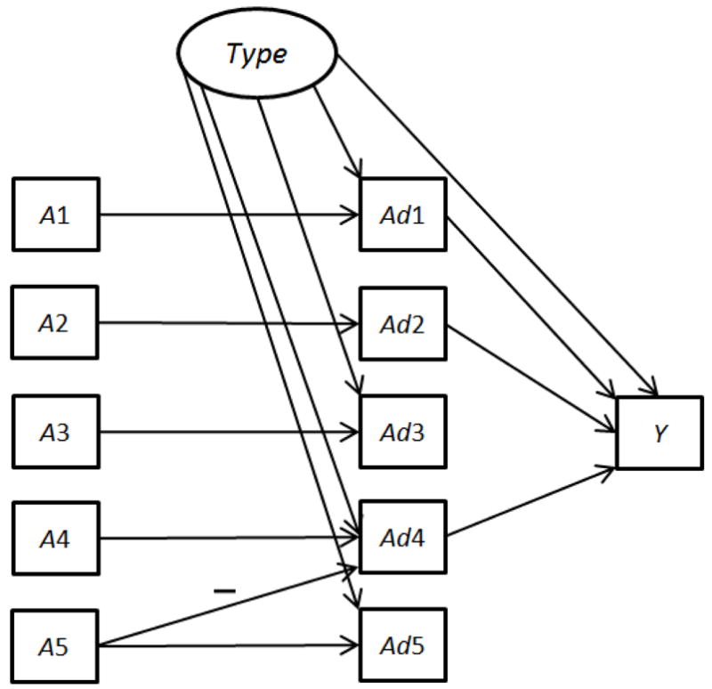
Data generation model for simulation.

Averaging over the distribution of Type and Ad1–Ad5 produces the marginal linear model

$$E[Y\mid A1,\dots ,A5]=c_0+c_{1}A1+c_{11}A{1}^2+c_{2}A2+c_{4}A4+c_{45}A4A5$$ (1)

Furthermore the variance of Y given A1,…, A5 is a function of the components A1,…, A5, that is, the variance is nonconstant (see Appendix A).

Experimental conditions

In the simulation there were three effect size conditions for the interventions, corresponding to Cohen’s [35] benchmark values for standardized effect sizes of small (d=.2), medium (d=.5) and large (d=.8). Effect sizes were defined in terms of the ideal intervention as a whole, in other words, for the two-group comparison of the best treatment combination (A1 set to medium, A2 and A4 included, A3 and A5 not included) versus a control group. Active main effects were roughly equal in magnitude, and the effect corresponding to the active interaction (A4A5) was roughly half the size of the main effects.¹ All other intervention component main effects and interactions were set to 0. Across all three effect size conditions, the effect of Type was set equal to d=0.9. For each of the three effect size conditions, 1000 simulated data sets of N=1200 random experimental subjects were generated. Each generated data set was used twice: once for the classical approach, and once for the experimental approach. All the results presented in Tables 1–3 are averages based on the 1000 simulated data sets.

Table 1.

Mean Intervention Outcome under Classical and Phased Experimental Approaches, Averaged over 1000 Simulated Datasets

Effect Size	E(Y)Classical (standard error)	E(Y)Phased Experimental (standard error)	Difference (standard error)	Maximum Possible E(Y)
Small	1.72 (.00)	1.69 (.01)	.03 (.01)	1.99
Medium	2.35 (.01)	2.58 (.01)	−.23 (.02)	2.99
Large	3.01 (.02)	3.75 (.01)	−.74 (.02)	4.00

Table 3.

Accuracy of Component Selection under Classical and Phased Experimental Approaches (Percentage of Data Sets)

Effect Size	Classical	Phased Experimental
Correct Combination of Components/Levels Identified
Small	1.9	7.5
Medium	3.7	24.3
Large	5.5	52.0
All Active Components Identified
Small	48.5	14.5
Medium	48.4	37.3
Large	48.2	73.5
All Inactive Components Identified
Small	20.0	45.7
Medium	19.5	61.0
Large	19.2	68.5

Operationalization of the classical and phased experimental approaches

This section contains a brief overview of the operationalizations of the classical and phased experimental approaches. A detailed description of the phased experimental approach can be found in Appendix B.

The classical approach

The classical approach employed all N=1200 experimental subjects in a single RCT of the multi-component treatment vs. control, followed by post hoc analysis. The treatment group was given an intervention consisting of A1 set to “high” and all of the other components included; the control group was given an intervention with A1 set to “low” and none of the other components included. Because only homogeneous subpopulations were considered in this simulation study (see the data generation model above), there were no pretreatment variables to be controlled. As is traditional, a two-group comparison was performed for the overall efficacy of the intervention. However, regardless of the outcome of this comparison, decisions about whether individual components should be retained in the intervention were based on post-hoc dose-response analyses (with the levels of adherence Ad1,…, Ad5 as doses) on the treatment group of subjects as follows:

Step 1: Identify components with sufficient variation in dose to enable dose-response analyses

Received dose (adherence) could vary between 0 and 2 for A1 and between 0 and 1 for A3–A5 (adherence was always 100 percent for A2, so there was no variation). Any components for which naturally occurring variation in dose was greater than an arbitrary threshold of 0.01 were considered to have sufficient variation to enable dose-response analyses. Any components with variation in dose less than 0.01 could not be examined further, and were automatically included in the final intervention.

Step 2: Multiple regression

The outcome Y was regressed on the following variables: doses of all components with sufficient variation in dose; two-way interactions between them; and, if Ad1 was included in the regression, a quadratic term for Ad1 (an implicit assumption here is that the scientist knows that A1 has more than two levels).

Step 3: Select components and levels

The estimated regression function was evaluated at each combination of levels of the components that had sufficient variation in dose (by plugging in possible values of A’s in place of Ad’s, e.g., 0, 1, or 2 for Ad1, and 0 or 1 for Ad3–Ad5). The level combination that produced the largest predicted value of Y was identified.

Step 4: Final intervention

The final intervention identified by the classical approach consisted of (a) the low-variation components identified in Step 1, each set to 1 (2 in the case of A1), plus (b) the configuration of components and levels identified in Step 3.

The phased experimental approach

The phased experimental approach used the same N=1200 subjects as the classical approach, but employed N=800 subjects in an initial screening phase of experimentation and reserved N=400 for a subsequent refining phase.

In the screening phase, a factorial experiment involving all five components was conducted, with only the low and the high levels of A1 included. To conserve resources, a 16-condition balanced fractional factorial design was used instead of a 32-condition complete factorial. (See Appendix B for a technical discussion about the particular choice of fraction and the rationale behind it.) This experiment was used to identify significant main effects and 2-way interactions.

Intervention components were selected based on the results of the screening phase using the following decision rules: First, any component with a significant main effect and not involved in a significant interaction was selected for inclusion in the intervention. A main effect was deemed significant if it possessed one of the three largest positive t-statistics or if the associated t-test was significant at the .10 level and positive. (The decision rule to take the three largest was arbitrary to an extent; below we summarize the results of additional simulations that varied this decision rule.) Interactions were deemed significant if the associated t-test was significant at the .10 level. Next, any components involved in significant two-component interactions were examined further. The combination of the two components that produced the highest marginal cell mean on Y was selected for inclusion. (This procedure is described in more detail in Appendix B.)

In this study the purpose of the refining phase was to determine the optimal value of A1. Therefore, if A1 and all its interactions were insignificant, the refining phase was not conducted. Otherwise, additional experimentation to revise the selected level for A1 was conducted as follows: (a) If the main effect of A1 was significant but no interactions were significant, the refining experiment was a two-group comparison of level 2 of A1 against level 1 of A1. In this experiment the remaining components were set at the levels indicated by the screening phase. The results of this experiment yielded the best level for A1. (b) If there were one or two significant interactions involving A1, a factorial experiment was conducted crossing A1 with the components involved in the interactions, with the remaining components set to the levels indicated by the screening phase. These results yielded the best levels for A1 and for the components that interacted with A1. (More detail appears in Appendix B.)

Evaluation of outcomes of each approach

Because in this simulation the true data generation model is known, it is possible to use this model to evaluate the performance of the classical and phased experimental approaches. After the final intervention was determined using either the classical or phased experimental approach, the data generation model was used to compute the expectation of the distribution of Y that would be obtained if the intervention were applied to all subjects in the population. These expectations, E(Y)_classical and E(Y)_{phased experimental}, were the outcome variables used to evaluate the performance of each approach. In real life this step would instead consist of conducting a large RCT comparing the final intervention to an appropriate control group (this is called the confirming phase of the phased experimental approach – see [19, 20, 24]).

Results

As was described above, the classical approach and the phased experimental approach each identifies a final multicomponent intervention for every simulated data set. The two final multicomponent interventions are then evaluated using the known data generation model. All the results presented in Tables 1–3 are averaged over the 1000 simulated data sets.

Table 1 shows the mean outcome of the classical and phased experimental approaches, the mean difference between them, and standard errors. For reference, the maximum possible mean outcome value is included. Table 1 shows that in the small effect size condition E(Y)_classical was approximately two percent larger than E(Y)_{phased experimental}, indicating that in this condition the average intervention outcome was slightly better for the classical approach. In the medium and large effect size conditions the average intervention outcome was about 10 and 25 percent larger, respectively, for the phased experimental approach. The difference between the classical and phased experimental approaches is significant at the 0.05 level in every condition.

Table 2 shows the percent of data sets in which each approach “won” by identifying an intervention that yielded a larger value of the outcome E(Y). In the small effect size condition the classical approach was about 1.3 times more likely than the phased experimental approach to identify an intervention that yielded a larger E(Y). In the medium and large effect size conditions the effect was reversed, with the phased experimental approach about 1.9 and 5.1 times more likely, respectively, to identify an intervention that yielded a larger E(Y).

Table 2.

Comparison of Classical and Phased Experimental Approaches on E(Y) (Percentage of Data Sets)

Effect Size	E(Y)Classical Higher	E(Y)Phased Experimental Higher	Neither Higher (tied)
Small	54.2	40.8	5.0
Medium	32.3	62.4	5.3
Large	14.9	75.7	9.4

Table 3 depicts the accuracy with which each approach selected intervention components and levels for inclusion in the intervention or identified components for exclusion. The first section of the table shows the percent of data sets in which the correct configuration of components and levels was identified. As expected, this number increased for both approaches as effect size increased. In every condition the phased experimental approach was much more likely to identify the correct configuration. One reason for the better performance of the experimental approach is that it identified the medium level of A1 as optimal more frequently than the classical approach (in 61.3 vs. 11.8 percent of data sets in the small effect size condition, 90.7 vs. 31.0 percent in the medium effect size condition, and 98.3 vs. 40.6 percent in the large effect size condition). Another reason is that the experimental approach included the component A5 (which, as described above, produced a subadditive effect in presence of the active component A4) in the intervention much less frequently (in 25.4 vs. 57.6 percent of data sets in the small effect size condition, 11.5 vs. 57.2 percent in the medium effect size condition, and 6.5 vs. 56.9 percent in the large effect size condition).

The second section of Table 3 shows the percentage of data sets in which all active components were correctly selected, irrespective of whether inactive components were mistakenly selected, and irrespective of the selected level of A1. The classical approach outperformed the phased experimental approach on this criterion for the small and medium effect size conditions. For the phased experimental approach the performance improved dramatically (from 14.5 to 73.5 percent) as the effect size increased. However, the performance of the classical approach was fairly constant (ranging from 48.2 to 48.5 percent) across the effect size conditions.

The third section of Table 3 shows the percentage of data sets in which all inactive components were correctly excluded, irrespective of whether some active intervention components were incorrectly excluded. Across all three effect size conditions the performance of the phased experimental approach was better than the classical approach. Here too performance improved as effect size increased for the phased experimental approach, but not for the classical approach.

Other sample sizes and numbers of main effects retained

We conducted some additional simulations in order to investigate whether the results reported here held across variation along two dimensions. One was sample size. The other was the decision rule used in the phased experimental approach for selecting intervention components for inclusion based on main effects estimates. In a series of nine simulations we investigated three different sample sizes, N=600, N=1200, and N=2500; and three different decision rules: retention of the intervention components corresponding to the largest two, three, and four main effects.

The overall pattern of results was very consistent. In general the classical approach tended to produce a larger E(Y) than the phased experimental approach in conditions involving both a small effect size and a small sample size. The phased experimental approach tended to produce a larger E(Y) than the classical approach in the medium and large effect size conditions, even in the small sample size condition. The phased experimental approach tended to produce larger E(Y) than the classical approach when the decision rule called for retaining a larger number of main effects; in the conditions in which the four largest main effects were retained the phased experimental approach consistently produced the larger E(Y), even in the conditions involving both a small effect size and a small sample size. More details can be found in Appendix C.

Discussion

The simulation reported here compared one possible operationalization of the phased experimental approach to one possible operationalization of the classical approach. Which approach performed best depended upon which criterion was used to evaluate the approaches and also upon intervention effect size.

When the two approaches were evaluated in terms of overall intervention outcome, the classical approach performed better than the phased experimental approach when the intervention effect size was small, and the phased experimental approach performed better than the classical approach when the intervention effect size was medium or large. The phased experimental approach suffered somewhat from a lack of statistical power in the small effect size condition. One reason why the classical approach tended to be outperformed by the phased experimental approach in the medium and large effect size conditions is confounding by the unknown participant characteristic Type. Type introduced a positive bias that had an impact on the results of the classical approach primarily in two areas. First, this positive bias made the high level of A1 look better than the medium level in the post-hoc dose-response analysis. Second, the positive bias also masked the subadditive effect of A5 on A4 in the post-hoc analysis, sometimes leading to the incorrect inclusion of the component A5. Type had little or no impact on the results of the phased experimental approach because this approach depended primarily on estimates of main effects and interactions based on data from randomized experiments, which are much less likely to be biased by confounding than are post hoc non-experimental analyses [36].

When success at identifying the best combination of components and levels was the criterion, the phased experimental approach was the better of the two across all effect sizes. This is directly due to the greater impact of confounding on the classical approach as compared to the phased experimental approach. For example, confounding by Type made the classical approach more likely to lead to choose an incorrect level of A1, as mentioned above, even though a quadratic term was appropriately included in regression analyses.

When the two approaches were evaluated in terms of successfully including all of the active components, the classical approach performed better than the phased experimental approach in the small and medium effect size conditions, and the phased experimental approach performed better when effect sizes were large. The phased experimental approach detected active components at a higher rate as effect size increased, due to the corresponding increase in statistical power. By contrast, the classical approach detected active components at a relatively constant rate across increasing effect sizes. The primary reason for this is that in our operationalization of the classical approach the components with low variability in adherence were automatically included, irrespective of effect size. For example, the active component A2 was always included because the received dose, Ad2, was always equal to the assigned value of A2 (100% adherence).

The phased experimental approach outperformed the classical approach in all effect size conditions when the criterion was successfully identifying inactive or potentially counterproductive components that should be eliminated from the intervention. Again, this is attributable to the differential impact of confounding. Because Type is positively associated with both Y and Ad’s, it induced a positive bias in the non-experimental analyses that led the classical approach to a preference for including components over excluding them.

Choosing an approach to intervention building

Our results suggest that when medium or large intervention effect sizes are anticipated use of a phased experimental approach is likely to result in identifying a more potent intervention than the classical approach. When a small intervention effect is anticipated, the choice is less clear. Multicomponent interventions with small overall effect sizes may be made up of either (a) mostly inactive components with one or two components with relatively large effect sizes, or (b) fairly equally efficacious but weak components, which together produce a detectable aggregate effect even though no individual component has a detectable effect. In situation (a), the phased experimental approach may be helpful in identifying the inactive components. In situation (b), in order to perform well the phased experimental approach would need to be powered to detect the weak individual component effects. Here the classical approach may be a better choice.

One drawback of the classical approach is that all subjects in the treatment arm receive all the components, and so the main effects of all the components and their interactions of every order are confounded (aliased). In contrast, in the phased experimental approach if a fractional factorial design is used main effects and two-way interactions are confounded with only higher order interactions deemed negligible in size, and hence do not affect the results. If a full factorial design is used there is no confounding of main effects and interactions.

It is possible that some other variant of the classical method (e.g., dismantling experiments, see [12]) would have performed better than the approach used in the simulation reported here. However, as long as post hoc analyses on non-randomized data (e.g., adherence) are used, the performance of any version of the classical method will depend on the degree of confounding present in the data. In situations in which the degree of confounding is very low or nonexistent, the version of the classical approach we have used and other reasonable variants would probably perform as well as the phased experimental approach. Of course, in most cases the degree and nature of confounding is not under the investigator’s control and may be difficult to anticipate. Because the phased experimental approach is entirely based on randomization, it is much less vulnerable to confounding.

Although the phased experimental approach was better overall at identifying the best configuration of components and levels, the success rate ranged from a high of 52 percent to a low of about 7.5 percent. Thus there is plenty of room for improvement, particularly when effect sizes are small. It is possible that an augmented approach or even an entirely different approach could result in a higher success rate. One promising avenue for intervention refinement may lie in exploring ideas from engineering process control, as discussed in Rivera et al. [37].

Differences in resource requirements

One question that arises in considering the phased experimental approach is whether the additional experimentation required by this approach necessarily demands an increase in cost over the classical approach. The phased experimental approach calls for a design that can isolate the effects of individual components. In the screening phase this will usually be some variation of a factorial design, requiring implementation of numerous conditions, each of which represents a different version of the intervention. For example, a full factorial design involving k two-level components requires implementation of 2^k treatment conditions, which may be costly. By contrast, irrespective of the number of components studied the classical approach typically requires implementation of only two conditions, a treatment and a control.

Two important costs are experimental subjects and implementation of experimental conditions. In this simulation the phased experimental approach used exactly the same number of experimental subjects as the classical approach, suggesting that it is no more demanding with respect to sample size. When a factorial design is used, given a fixed number of subjects an investigator may test as many components as desired – the power to detect every main effect in this way is about the same as testing that component in a single-component 2-arm study with the same sample size. This means that factorial experiments make very efficient use of experimental subjects. Power and sample size considerations (e.g., for testing main effects) in a factorial setting can be found in Byar and Piantadosi [38], Byth and Gebski [39], Green et al. [40], and Montgomery et al. [41].

However, even when in the phased experimental approach the same number of subjects is used as in a comparable classical approach, there may be additional costs associated with implementing a wider variety of versions of the intervention and conducting follow-up experiments. It may also take more time to implement the phased experimental approach, and may require more training of intervention delivery staff. Although these logistics and costs associated with the phased experimental approach are a serious consideration, highly efficient fractional factorial designs offer a way to keep the number of experimental conditions manageable. Some assumptions about higher-order interactions being negligible are necessary in order to take advantage of the economy offered by a fractional factorial over a full factorial design. The particular fractional design used in the simulations reported here did not allow estimation of 3-way or higher order interactions; instead, it required the assumption that they are negligible in size. Many fractional factorial designs are available. If prior knowledge suggests that some 3-way interactions can be important, an investigator can choose a different fractional design that allows estimation of 3-way interactions (see [28]).

Even with a highly efficient design investigators in empirical settings sometimes have to make decisions based on results of past studies and auxiliary analysis performed on data from the current study. This is particularly true when numerous interactions are anticipated. An example of such an analysis can be found in Strecher et al. [22].

The short-term costs of building and evaluating an intervention must be weighed against long-range costs and benefits. Our results suggest that the phased experimental approach may help identify more efficient and streamlined interventions by identifying inactive components for elimination. As Allore et al. [1] noted, “Since each component of an intervention adds to the overall cost and complexity, being able to directly estimate component effects could greatly enhance efficiency by reducing the number of components introduced into clinical practice” (p. 14). Our results also suggest that under many circumstances the phased experimental approach may be likely to identify a more efficacious intervention than the classical approach. Thus, in some applications the long-range gains in terms of increased efficiency and public health benefits expected to result from the phased experimental approach may offset any additional up-front intervention development costs.

Limitations

This simulation was designed to take an initial look at the question of whether a phased experimental approach is a reasonable way to build interventions. It involved only a very small set of conditions out of the infinite number of possibilities that can occur in practice. There are a number of potentially important factors that were not varied in the simulation. A few of these are: the underlying structural model, which could be varied to include features such as more 2-way interactions, higher-order interactions, and the presence of mediating variables; the degree of confounding, here reflected by the variable Type; the number of components under consideration; the number of active vs. inactive components; other effect sizes besides the three used here; the impact of measurement noise on the outcome variable; the effect of complex data structures such as nesting (e.g. individuals within classrooms; patients within clinics); incorporating cost and burden in decisions about which components and levels should make up an intervention; and the operationalization of the classical approach used. Many other additional factors could be considered. Despite the limitations of this study and the need for additional research, we believe that the results of the simulation show clearly that the phased experimental approach is a promising alternative.

Conclusions

The classical approach is currently the most well-established approach to empirical development of behavioral interventions. However, an emergent strategy, labeled here the phased experimental approach, provides a systematic way of making evidence-based decisions about which components and which component levels should comprise an intervention. Comparison of the two approaches in real-world empirical settings is impractical. In the present article a simulation was presented that provides this comparison by modeling a plausible empirical scenario. The results suggested that the phased experimental approach merits serious consideration, because it has the potential to help intervention scientists to build more potent behavioral interventions. Possible exceptions to this are interventions with a small overall effect size, particularly those that are the cumulative effect of many weak components. More research is needed on methods to identify the optimal intervention, and thereby increase public health benefits.

References

- 1.Allore HG, et al. Experimental designs for multicomponent interventions among persons with multifactorial geriatric syndromes. Clinical Trials. 2005;2(1):13–21. doi: 10.1191/1740774505cn067oa. [DOI] [PubMed] [Google Scholar]
- 2.Campbell M, et al. Framework for design and evaluation of complex interventions to improve health. British Medical Journal. 2000;321:694–696. doi: 10.1136/bmj.321.7262.694. [DOI] [PMC free article] [PubMed] [Google Scholar]
- 3.Craig P, et al. Developing and evaluating complex interventions: The new Medical Research Council guidance. British Medical Journal. 2008;337:a1655. doi: 10.1136/bmj.a1655. [DOI] [PMC free article] [PubMed] [Google Scholar]
- 4.Williams JW, et al. Systematic review of multifaceted interventions to improve depression care. General Hospital Psychiatry. 2007;29:91–116. doi: 10.1016/j.genhosppsych.2006.12.003. [DOI] [PubMed] [Google Scholar]
- 5.Rush AJ, et al. Acute and longer-term outcomes in depressed outpatients who required one or several treatment steps: A STAR*D report. American Journal of Psychiatry. 2006;163(11):1905–1917. doi: 10.1176/ajp.2006.163.11.1905. [DOI] [PubMed] [Google Scholar]
- 6.Cuffe M. The patient with cardiovascular disease: treatment strategies for preventing major events. Clinical Cardiology. 2006;29:II4–12. doi: 10.1002/clc.4960291403. [DOI] [PubMed] [Google Scholar]
- 7.Cofta-Woerpel L, Wright KL, Wetter DW. Smoking cessation 3: multicomponent interventions. Behavioral Medicine. 2007;32:135–149. doi: 10.3200/BMED.32.4.135-149. [DOI] [PubMed] [Google Scholar]
- 8.Golin CE, et al. A 2-arm, randomized, controlled trial of a motivational interviewing-based intervention to improve adherence to antiretroviral therapy (ART) among patients failing or initiating ART. Journal of Acquired Immune Deficiency Syndrome. 2006;42:42–51. doi: 10.1097/01.qai.0000219771.97303.0a. [DOI] [PMC free article] [PubMed] [Google Scholar]
- 9.Bluford DA, Sherry B, Scanlon KS. Interventions to prevent or treat obesity in preschool children: A review of evaluated programs. Obesity. 2007;15:1356–1372. doi: 10.1038/oby.2007.163. [DOI] [PubMed] [Google Scholar]
- 10.Narayan KM, Kanaya AM, Gregg EW. Lifestyle intervention for the prevention of type 2 diabetes mellitus: putting theory to practice. Treatments in Endocrinology. 2003;2:315–320. doi: 10.2165/00024677-200302050-00003. [DOI] [PubMed] [Google Scholar]
- 11.COMBINE Study Research Group. Testing combined pharmacotherapies and behavioral interventions in alcohol dependence: Rationale and methods. Alcoholism: Clinical and Experimental Research. 2003;27:1107–1122. doi: 10.1097/00000374-200307000-00011. [DOI] [PubMed] [Google Scholar]
- 12.West SG, Aiken LS, Todd M. Probing the effects of individual components in multiple component prevention programs. American Journal of Community Psychology. 1993;21:571–605. doi: 10.1007/BF00942173. [DOI] [PubMed] [Google Scholar]
- 13.Wolchik SA, et al. The children of divorce intervention project: Outcome evaluation of an empirically based parenting program. American Journal of Community Psychology. 1993;21:293–331. doi: 10.1007/BF00941505. [DOI] [PubMed] [Google Scholar]
- 14.Conduct Problems Prevention Research Group. Initial impact of the Fast Track prevention trial for the prevention of conduct disorders: I. The high risk sample. Journal of Consulting and Clinical Psychology. 1999;67:631–647. [PMC free article] [PubMed] [Google Scholar]
- 15.Conduct Problems Prevention Research Group. Initial impact of the Fast Track prevention trial for the prevention of conduct disorders: II. Classroom effects. Journal of Consulting and Clinical Psychology. 1999;67:648–657. [PMC free article] [PubMed] [Google Scholar]
- 16.Riggs N, Elfenbaum P, Pentz M. Parent program component analysis in a drug abuse prevention trial. Journal of Adolescent Health. 2006;39:66–72. doi: 10.1016/j.jadohealth.2005.09.013. [DOI] [PubMed] [Google Scholar]
- 17.Tinetti ME, et al. A multifactorial intervention to reduce the risk of falling among elderly people living in the community. New England Journal of Medicine. 1994;331:821–827. doi: 10.1056/NEJM199409293311301. [DOI] [PubMed] [Google Scholar]
- 18.Tinetti ME, McAvay G, Claus EB. Does multiple risk factor reduction explain the reduction in fall rate in the Yale FICSIT trial? American Journal of Epidemiology. 1996;144:389–399. doi: 10.1093/oxfordjournals.aje.a008940. [DOI] [PubMed] [Google Scholar]
- 19.Collins LM, et al. A strategy for optimizing and evaluating behavioral interventions. Annals of Behavioral Medicine. 2005;30:65–73. doi: 10.1207/s15324796abm3001_8. [DOI] [PubMed] [Google Scholar]
- 20.Collins LM, Murphy SA, Strecher V. The Multiphase Optimization Strategy (MOST) and the Sequential Multiple Assignment Randomized Trial (SMART): New methods for more potent e-health interventions. American Journal of Preventive Medicine. 2007;32:S112–S118. doi: 10.1016/j.amepre.2007.01.022. [DOI] [PMC free article] [PubMed] [Google Scholar]
- 21.Fagerlin A, et al. Society for Medical Decision Making. Cambridge, MA: 2006. Decision aid design influenced patients’ knowledge, risk perceptions, and behavior. [Google Scholar]
- 22.Strecher VJ, et al. Web-based smoking cessation components and tailoring depth: Results of a randomized trial. American Journal of Preventive Medicine. 2008;34:373–381. doi: 10.1016/j.amepre.2007.12.024. [DOI] [PMC free article] [PubMed] [Google Scholar]
- 23.Hosking JD, et al. Design and analysis of trials of combination therapies. Journal of Studies on Alcohol. 2005;(Supplement15):34–42. doi: 10.15288/jsas.2005.s15.34. [DOI] [PubMed] [Google Scholar]
- 24.Nair V, et al. Screening experiments and fractional factorial designs in behavioral intervention research. American Journal of Public Health. 2008;98:1354–1359. doi: 10.2105/AJPH.2007.127563. [DOI] [PMC free article] [PubMed] [Google Scholar]
- 25.Box GEP, Draper NR. Empirical model-building and response surfaces. New York: Wiley; 1987. [Google Scholar]
- 26.Box GEP, Hunter WG, Hunter JS. Statistics for experimenters: An introduction to design, data analysis, and model building. New York: Wiley; 1978. [Google Scholar]
- 27.Myers RH, Montgomery DC. Response surface methodology. New York: Wiley; 1995. [Google Scholar]
- 28.Wu CFJ, Hamada M. Planning, analysis, and parameter design optimization. New York: Wiley; 2000. [Google Scholar]
- 29.Rukshin V, et al. A prospective, non-randomized, open-labeled pilot study investigating the use of magnesium in patients undergoing nonacute percutaneous coronary intervention with stent implantation. Journal of Cardiovascular Pharmacology and Therapeutics. 2003;8:193–200. doi: 10.1177/107424840300800304. [DOI] [PubMed] [Google Scholar]
- 30.Korn EL, Teeter DM, Baumrind S. Using explicit clinician preferences in nonrandomized study designs. Journal of Statistical Planning and Inference. 2001;2001:67–82. [Google Scholar]
- 31.Vogt WP. Dictionary of statistics and methodology: A nontechnical guide for the social sciences. Newbury Park, CA: SAGE; 1993. [Google Scholar]
- 32.Strecher V, Shiffman S, West R. Randomized controlled trial of a web-based computer-tailored smoking cessation program as a supplement to nicotine patch therapy. Addiction. 2005;(100):682–688. doi: 10.1111/j.1360-0443.2005.01093.x. [DOI] [PubMed] [Google Scholar]
- 33.Rush AJ, et al. Texas Medication Algorithm Project, phase 3 (TMAP-3): Rationale and Study Design. Journal of Clinical Psychiatry. 2003;64(4):357–369. doi: 10.4088/jcp.v64n0402. [DOI] [PubMed] [Google Scholar]
- 34.Pearl J. Graphs, causality, and structural equation models. Sociological Methods and Research. 1998;27(2):226–284. [Google Scholar]
- 35.Cohen J. Statistical power analysis for the behavioral sciences. Mahwah, NJ: Lawrence Erlbaum Associates; 1988. [Google Scholar]
- 36.Shadish WR, Cook TD, Campbell DT. Experimental and quasi-experimental designs for generalized causal inference. Boston: Houghton Mifflin; 2002. [Google Scholar]
- 37.Rivera DE, Pew MD, Collins LM. Using engineering control principles to inform the design of adaptive interventions: a conceptual introduction. Drug and Alcohol Dependence. 2007;88:S31–S40. doi: 10.1016/j.drugalcdep.2006.10.020. [DOI] [PMC free article] [PubMed] [Google Scholar]
- 38.Byar DP, Piantadosi S. Factorial designs for randomized clinical trials. Cancer Treatment Reports. 1985;(69):1055–1063. [PubMed] [Google Scholar]
- 39.Byth K, Gebski V. Factorial designs: a graphical aid for choosing study designs accounting for interaction. Clinical Trials. 2004;1:315–325. doi: 10.1191/1740774504cn026oa. [DOI] [PubMed] [Google Scholar]
- 40.Green S, Liu P, O’Sullivan J. Factorial design considerations. Journal of Clinical Oncology. 2002;20:3424–3430. doi: 10.1200/JCO.2002.03.003. [DOI] [PubMed] [Google Scholar]
- 41.Montgomery AA, Peters TJ, Little P. Design, analysis and presentation of factorial randomised controlled trials. BMC Medical Research Methodology. 2003;3:26. doi: 10.1186/1471-2288-3-26. [DOI] [PMC free article] [PubMed] [Google Scholar]
Associated Data
This section collects any data citations, data availability statements, or supplementary materials included in this article.