

Abstract
In many cell types, the inositol trisphosphate receptor is one of the important components controlling intracellular calcium dynamics, and an understanding of this receptor is necessary for an understanding of calcium oscillations and waves. Based on single-channel data from the type-I inositol trisphosphate receptor, and using a Markov chain Monte Carlo approach, we show that the most complex time-dependent model that can be unambiguously determined from steady-state data is one with three closed states and one open state, and we determine how the rate constants depend on calcium. Because the transitions between these states are complex functions of calcium concentration, each model state must correspond to a group of physical states. We fit two different topologies and find that both models predict that the main effect of [Ca2+] is to modulate the probability that the receptor is in a state that is able to open, rather than to modulate the transition rate to the open state.
Introduction
The modulation of free Ca2+ concentration is a regulator of numerous physiological processes, including saliva secretion, muscle contraction, and cell division (1). The changes in the Ca2+ concentration involve interaction between the mechanisms controlling Ca2+ flux across the plasma membrane and across internal cell compartment membranes such as the endoplasmic reticulum (ER). In many cell types, Ca2+ release is via the inositol trisphosphate receptor, IPR, which is regulated by Ca2+ and inositol 1,4,5-trisphosphate, IP3, and other ligands (2). The release of Ca2+ from the ER can further modulate the open probability of the channel, resulting in complex Ca2+ oscillations and waves. Therefore, an understanding of the IPR dynamics is central to a detailed understanding of Ca2+ dynamics.
IPR can be studied using patch-clamp techniques (3) to record their single-channel activity. Early single-channel measurements were performed in lipid bilayers (4,5) and thus, not in their natural environment. However, recently it has been reported that the receptors are expressed in limited numbers in the plasma membrane of DT40 cells (6,7), such that their activity can be measured using the whole-cell mode of the patch-clamp technique. As the receptor is localized such that a normal orientation in the cytoplasm is retained, it might be expected that the IPR is regulated in a relatively normal manner. The plasma membrane lipid environment is also likely to be similar to the ER membrane. Thus, it is now possible to measure single-channel activity of an IPR in an environment that is, presumably, relatively similar to its native environment.
The open probability of the IPR at steady state is a bell-shaped function of the Ca2+ concentration (5) and this has been a central feature in many models of the IPR (8–13). However, kinetic properties of the receptor are also important. After a step increase in Ca2+ concentration, the IPR flux, measured by labeled flux experiments, first increases and then decreases (14–17). This time-dependent data is fitted by Sneyd and Dufour (18). A review of different IPR models can be found in Sneyd and Falcke (19).
During realistic Ca2+ oscillations and waves, the IPR is rarely at steady state, and so to understand the behavior and function of the IPR, it is crucial to construct models that have both the correct steady-state properties as well as the correct time dependence. However, this has proven difficult. Although single-channel recordings are excellent at obtaining steady-state data, it is considerably more difficult to determine kinetic behavior from single-channel measurements. Conversely, although labeled flux experiments can give a clear picture of time-dependent behavior, they suffer from their own disadvantages; questions such as luminal depletion and possible buildup around the mouth of a channel can make interpretation of the results problematic.
Our goal here is to develop a minimal Markov model of an IPR, based solely on steady-state single-channel measurements. In doing so, we develop the simplest possible time-dependent model of the IPR (consistent with our experimental data), but avoid the perils of interpretation associated with labeled flux experiments. The most important question is: given the available data, how precisely may the kinetic rate constants be determined, and what is the most complex model for which all the rate constants may be determined unambiguously? We fit two topologies with the same number of open and closed states and investigate the type of data needed to distinguish between the two models.
Steady-state single-channel data were obtained from the type-1 IPR at various Ca2+ concentrations at a single, presumably saturating [IP3]. Thus, we are able to determine how the rate constants in the minimal model depend on Ca2+ concentrations and investigate how the open probability is affected by Ca2+.
Here we use a Bayesian inference and a Markov chain Monte Carlo (MCMC) method developed by Ball et al. (20) to fit directly to experimental single-channel data. In theory, the fit will determine both the rate constants of the underlying Markov model as well as the sequence of openings and closings, although, as shall be seen, the actual process can be made somewhat simpler in practice. For more-extensive fitting details, see Gin et al. (21).
Methods
Electrophysiology
All experiments were performed in chicken DT40-3KO cells engineered to stably express rat S1-/S2+ IPR-1. Because endogenous IPRs have been genetically deleted in the DT4-3KO cell type, stable expression of the expressed mammalian IPR allows its study in unambiguous isolation. All experiments were performed using the whole-cell configuration of the patch-clamp technique, which allows the measurement of single channel activity from IPR present in the plasma membrane as previously described (6,7).
K+ was utilized as the charge carrier in all experiments. The bath contained; 140 mM KCl, 10 mM HEPES, 500 μM BAPTA, and free Ca2+ 250 nM at pH 7.1. The pipette contained 100 μM IP3, 140 KCl mM, 10 mM HEPES, 100 μM BAPTA, 0.5 mM ATP, and free Ca2+ as indicated at pH = 7.1. Pipette [Ca2+] was calculated using MaxChelator and verified by fluorimetry. The ATP was in the form of Na+ ATP. Borosilicate glass pipettes were pulled and fire-polished to resistances of ∼20 MΩ. Following establishment of stable high resistance seals, the membrane patches were ruptured to form the whole-cell configuration with resistances >5 GΩ and capacitances >8 pF. The holding potential was set to −100 mV during the recording, except where noted, and currents were recorded under voltage-clamp conditions using an Axopatch 200B amplifier and pClamp 9. Channel recording were digitized at 20 kHz and filtered at 5 kHz with a −3 dB, four-pole Bessel filter.
Representative examples of channel activity are shown in Fig. 1 at different values of [Ca2+] with an [IP3] of 100 μM.
Figure 1.
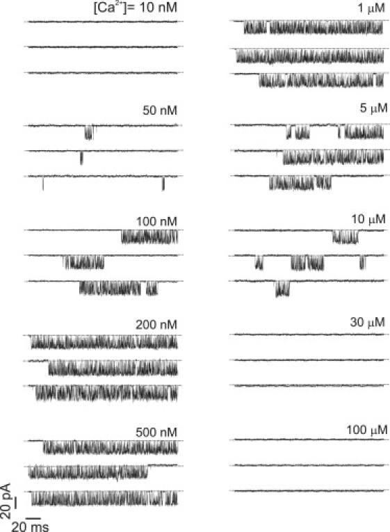
Whole-cell patch-clamp recordings of single-channel activity for various [Ca2+] obtained at a saturating [IP3] of 100 μM.
Fitting methods
We will use Bayesian inference and Markov chain Monte Carlo (22) methods to fit the rate constants. A detailed description of the method as given in Gin et al. (21). Here, we give only a very brief description. The parameter distributions are obtained by sampling appropriately from an a posteriori distribution. Given parameters q, and data x, the posterior probability distribution is given by
| (1) |
where p(·|·) denotes a conditional probability. The left-hand side of Eq. 1 is the quantity in which we are interested, with the maximum of p(q|x) giving the set of rate constants that maximizes the probability of obtaining the observed data. We do not take this maximization approach, but instead construct the entire distribution from which we can extract any statistical quantity required, such as the maximum or mean, by using MCMC techniques. Details of the terms on the right-hand side of Eq. 1 are given in Gin et al. (21).
The data, x, used to fit the model, are the durations of the open times and closed times. To obtain the set of open times and closed times a threshold algorithm is applied to the single-channel record. A threshold is set at 50% of the mean open current and everything below the threshold is considered closed, while everything above the threshold is considered open. The distribution of the closed time and open time durations are then plotted in a histogram, examples of which are shown later in Fig. 3, A and B. It is usually more convenient to look at the logarithm of the time given the wide range of timescales (23). The theoretical distributions of the open and closed times can then be approximated by sums of decaying exponentials, which are not model-specific, or if given a Markov model, it is a relatively simple matter to calculate the theoretical distributions of the open and closed times (24,25). By fitting to these experimentally determined open time and closed time probability distribution functions, the parameters of the Markov model may be determined.
Figure 3.
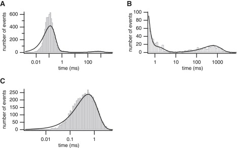
Experimental distributions for one experiment at 50 nM [Ca2+] and 100 μM [IP3]. (A) Closed time distribution. (B) Enlargement of the closed time distribution between 0.5 ms and 8000 ms. (C) Open time distribution. Fitted theoretical distributions superimposed.
The limited time resolution of the experimental recording means very brief opening and closing events will go undetected. There are a number of ways to correct for missed events (26–28). The approximation of Blatz and Magleby (26) is one of the simplest and is reasonably accurate, as long as the rate constants of the Markov model are not too large. This method assumes that missed events only occur for transitions from open to closed and closed to open. We use the Blatz and Magleby (26) method to correct for missed events.
Data fitted
Data were obtained at 10 Ca2+ concentrations, shown in Fig. 1. At Ca2+ concentrations of 10 nM, 30 μM, and 100 μM, no activity was evident during the recordings. For each concentration, single-channel data was obtained for five or six cells in each condition, representing between 8 and 29 min of experimental recordings for each case.
On examining the data, we find two records at 1 μM [Ca2+], which clearly show different levels of activity within the single recording. One such set of data is shown in Fig. 2. Fig. 2 B shows a nine-second section of a much longer recording, which shows the transition from high to low open probability. To model such data, it would be necessary to use, essentially, two different Markov models, each with a different set of rate constants, and then include switching between the models. Furthermore, characterization of the statistics of the switching process would require a large number of observations of a switch. No such data are available, as a switch was observed only a very small number of times. It follows that, although our simple model can reproduce the averaged statistics of the two sections, it cannot reproduce such an abrupt switch between the two activity levels. However, this behavior is obvious in only two cells. Additionally, to account for two levels of activity, two open states are required (29), but on plotting the open time histograms, only one open state is evident. Therefore, we will only fit the higher open probability section of the record. This will be discussed at greater length in the last section.
Figure 2.
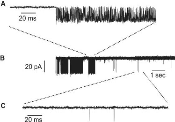
Single-channel activity at 1000 nM [Ca2+] 100 μM [IP3]. Panels A and C show expanded portions from panel B. Panel A shows much higher activity than panel C.
Results
The most complex identifiable model
To determine the number of states we should include in our Markov model, we plot the experimental steady-state closed-time and open-time distributions in logarithmically binned histograms (23), in Fig. 3, A–C. Only one distinct time constant can be seen in the open-time distribution (Fig. 3 B). For the closed-time distributions (Fig. 3, A and B), two distinct peaks are seen, corresponding to two distinct time constants, one of very short duration, at ∼0.1 ms, and another of very long duration, at ∼500 ms. This suggests that we should first consider models with one open state and two closed states.
However, we also tried fitting a model with three closed states and found that the data contain enough information to allow for the unambiguous determination of the rate constants associated with three closed states. The distribution fits are shown in Fig. 3. Fig. 3 B shows an enlargement of part of the closed-time distribution in Fig. 3 A, with a third peak fitted at ∼1 ms. We can calculate, from the fitted rate constants, the time constants for the three closed times: 0.123 ms, 1.06 ms, and 619.31 ms. The proportions of the number of events at each time constant can also be calculated and are 0.93, 0.033, and 0.038, respectively.
Two different configurations with one open state and three closed states are shown in Fig. 4. The kinetic rate constants are given by q with qij the rate constant from state i to j. All topologies are equivalent, giving the same steady-state behavior (30). We will discuss how to distinguish between equivalent models in the last section.
Figure 4.
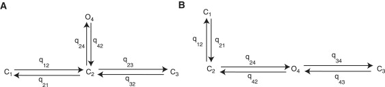
Two four-state Markov models. Closed states are C1, C2, C3; open state is O4. Kinetic rate constants given by qij; the transition from state i to j.
An example of a convergence plot and marginal histogram for rate constants q24 (by fitting the experimental data) from the first model is shown in Fig. 5. The convergence plot shows the rate constant has converged (after the burn-in period) and the marginal histogram shows a distinct peak corresponding to a mean of 7.57 pA with standard deviation 0.096 pA. All other rate constants converged similarly to a distinct mean and narrow variance.
Figure 5.
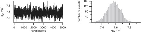
Rate constant convergence. Convergence plot and marginal histogram.
The fits in Fig. 3 show that the model predicts more short events than are obtained from the experimental data, which is constrained by the limited time resolution. This is compensated for by decreased peaks (as the total area must remain the same). However, the position of the peaks agrees very well with those of the measured histograms. Events shorter than the sampling resolution can be obtained as we sample the transitions between openings and closings (and vice versa) by selecting from the uniform distribution on the interval [0,0.05] (for details, refer to (21)). Our fits can be used to give a prediction of the number of short events that cannot be observed experimentally.
We have shown in previous work (21) that adding additional states or transitions between the states leads to ambiguity in the rate constants. Instead we find only convergence of the products and ratios of the rate constants. We concluded that nonconvergence of the rate constants is a strong indicator that the model is too complex. Thus, one can always add multiple states to a model, but not all rate constants can be identified, making the additional states essentially pointless. To identify the rate constants in a more complex model, additional data is required. In the experiments of Mak et al. (31), the [Ca2+] and [IP3] were changed rapidly, allowing the recording of the responses to these changes, in particular the activation and deactivation latency times. We showed previously that this could be used to determine a more complex model. For our experimental fits, however, we have only steady-state data available, constraining the number of identifiable states in our model and thus, we can fit only four-state models. We will show in a later section that this type of non-steady-state data could also be used to distinguish between different topologies with the same number of open and closed states.
We conclude that a four-state model (Fig. 4), with three closed states, one open state, and four transitions, is the most complex identifiable model that can be determined from the steady-state data.
Dependence on calcium
We first fitted the four-state model shown in Fig. 4 A (Model 1). Fig. 6, A–F, shows the mean fitted rate constants for the WT IPR at each Ca2+ concentration. There is a strong biphasic Ca2+ dependency for q23 and q32 (Fig. 6, C and D), but q12 and q21 appear to be independent of Ca2+. The dependency on Ca2+ of the transitions between the closed and open states, q24 and q42, also seem to be constant. To fit the steady-state data, it is sufficient to assume that the four rate constants q12, q21, q24, and q42 are constants and fit biphasic [Ca2+] dependencies only to q23 and q32 (shown by the curves).
Figure 6.
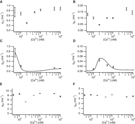
Fitted rate constants and [Ca2+] dependencies for Model 1. Standard deviations are shown.
Letting c = [Ca2+], the [Ca2+]-dependent fits are given by
| (2) |
| (3) |
Parameter values for these functions are given in Table 1.
Table 1.
Ca2+-dependent rate constant parameter values for Model 1
| V23 | 1.08 × 10⁶ nM2 ms−1 | k23 | 2000 nM | b23 | 2.2 ms−1 |
| V−23 | 0.3545 | k−23 | 72 nM | b−23 | 0.042 |
| a23 | 1/1.023 ms−1 | ||||
| V32 | 7 × 10⁶ nM3 ms−1 | k32 | 520 nM | b32 | 0.005 ms−1 |
| V−32 | 1.06 | k−32 | 150 nM | b−32 | 0.03 |
The mean fitted values for q23 at 200 nM and 500 nM are 0.0028 ms−1 and 0.0030 ms1, respectively—two orders-of-magnitude less than the value at 50 nM. There is a similar order-of-magnitude difference in the values of q32 over the concentration range. These two rate constants have a much more significant change in their values than the other rate constants.
To find the model steady-state open probability, mass action kinetics is used to give the system of differential equations governing the state dynamics. The steady-state solution is found by setting the system of differential equations equal to zero. The analytic expression for the steady-state open probability is
| (4) |
We use Eq. 4 to find the steady-state open probability curve (Fig. 7). The rate constants q23 and q32 are functions of [Ca2+], given by Eqs. 2 and 3; these biphasic functions produce the biphasic steady-state open probability curve. We set q12 = 0.74 ms−1, q21 = 0.11 ms−1, q24 = 7.84 ms−1, and q42 = 3.60 ms−1 (the mean values). The bars are the mean open probabilities calculated by using the individual fitted rate constants for each cell at each concentration. Standard deviations are also shown; these are calculated using a pooled standard deviation formula (see Supporting Material).
Figure 7.
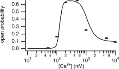
Steady-state open probability curve found from the fitted biphasic [Ca2+]-dependency curves. Bars give the mean fitted open probability calculated from the individual concentrations fits at each Ca2+ concentration.
The results from this model show clearly that the biphasic nature of the open probability is caused directly by changes in q23 and q32. Thus, the increasing open probability is due solely to the receptor being in a state that can open (C2), rather than an increased rate constant from C2 to O4.
We then fitted the model in Fig. 4 B with the open state separating the closed states (Model 2). For these fits, we found that the main route between closing and opening of the receptor is the transition between C3 and O4, with C3 corresponding to the shortest closed times. The fitted rate constants at each [Ca2+] concentration are shown in Fig. 8.
Figure 8.
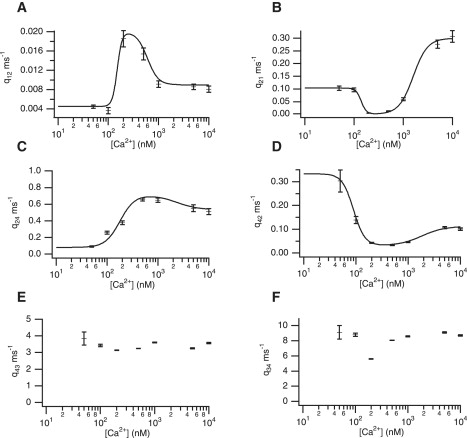
Fitted rate constants and [Ca2+] dependencies for Model 2. Standard deviations are shown.
The rate constants q43 and q34 are clearly Ca2+-independent, and we set these rates at their mean values of 3.52 and 8.43, respectively. The rate constants q24 and q42 show clear evidence of a biphasic dependency. However, it appears that q12 and q21 also might have a nonconstant dependency. Therefore we fit q12, q21, q24, and q42 with biphasic functions (shown in Fig. 8). The fits are given by
| (5) |
| (6) |
| (7) |
| (8) |
Parameter values for these functions are given in Table 2.
Table 2.
Ca2+-dependent rate constant parameter values for Model 2
| V12 | 9.2 × 10⁸ nM4 ms−1 | k12 | 600 nM | b12 | 0.0058 ms−1 |
| V−12 | 1.2 | k−12 | 150 nM | b−12 | 0.35 |
| V21 | 7.3 × 10⁸ nM3 ms−1 | k21 | 1600 nM | ||
| V−21 | 0.58 | k−21 | 140 nM | b−21 | 1.1 |
| a21 | 0.3 ms−1 | ||||
| V24 | 4 × 10⁶ nM2 ms−1 | k24 | 2300 nM | b24 | 2.2 ms−1 |
| V−24 | 0.215 | k−24 | 180 nM | b−24 | 0.027 |
| V42 | 8 × 10⁵ nM2 ms−1 | k42 | 1820 nM | b42 | 0.65 ms−1 |
| V−42 | 0.34 | k−42 | 90 nM | ||
| a42 | 1/3 ms−1 |
Rate constants q43 and q34 are set at their mean values of 3.52 and 8.43, respectively.
We then calculated, using the mean fitted rate constants at each concentration, the steady-state open probability (the corresponding analytic expression can be found for this model). The mean values are plotted along with the standard deviations in Fig. 9. Using the four biphasic curves, we calculated the open probability curve, giving the solid curve in Fig. 9. This gives a similar biphasic response as Model 1.
Figure 9.
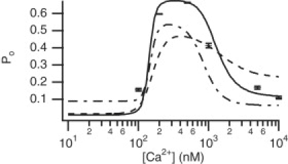
Steady-state open probability curve found from the fitted biphasic [Ca2+]-dependency curves for Model 2. Bars give the mean fitted open probability calculated from the individual concentrations fits at each Ca2+ concentration. (Solid curve) Biphasic functions for q12, q21, q24, and q42 used. (Dashed curve) Biphasic functions for q24 and q42, with q12 and q21 fixed at their mean values. (Dashed-dotted curve) Biphasic functions for q12 and q21, with q24 and q42 fixed at their mean values.
A minimal set of biphasic Ca2+-dependent functions that are needed to obtain the correct steady-state open probability behavior was investigated. We first fixed q12 and q21 at their mean values of 0.0095 and 0.13, respectively, and used the biphasic functions for q24 and q42 (dashed curve in Fig. 9). We did the same with q24 and q42 fixed at their mean values of 0.46 and 0.11, respectively, with biphasic functions for q12 and q21 (dashed-dotted curve). Clearly, using biphasic functions for all four rate constants gives a closer fit to the squares. Fig. 9 suggests that if a minimal set of Ca2+-dependencies is required, the rate constants q12 and q21 should be biphasic. Qualitatively, the shape of the open probability curve is much closer to the curve using the full set of Ca2+-dependencies.
The most obvious difference between Models 1 and 2 is that in Model 2, Ca2+ affects the closed-open transition directly via C2-O4. However, closer inspection shows that the C3-O4 transition is not affected. This transition corresponds to the main route between closed and open states with the mean closed time for C3 being the shortest of the three closed times. This feature is also found in Model 1 in which the main route was also not affected by Ca2+. For both models, the longest closed time is affected by Ca2+ (transitions involving C3 for Model 1 and C1 for Model 2). Therefore we can say that the main effect of [Ca2+] is to affect the route to the closed state, which is the main gateway to opening. In the case of Model 2, the receptor starts in state C1, and must arrive in C3 to obtain the rapid transitions between closed and open states.
Distinguishing between equivalent steady-state models
Both models fitted the steady-state single-channel data equally well, with little difference in their likelihoods. This raises the question as to what type of data could be used, in addition, to determine which model is more likely.
We investigated whether we could use non-steady-state data to distinguish between equivalent steady-state models. To do this, we simulated activation latency data from our two models using the mean fitted rate constants. We first started with the [Ca2+] at 50 nM, and then stepped-up the concentration to 200 nM. We assumed the receptor was at steady state at 50 nM, and therefore calculated the steady-state occupancies for each of the four states at this concentration. For Model 1, the steady-state occupancy is and for Model 2, . We then used the Gillespie algorithm to simulate ∼1000 times to first opening after an increase to 200 nM [Ca2+]. The distribution of the times to first opening is plotted in Fig. S1 in the Supporting Material, with the theoretical probability distribution functions, calculated from the fitted rate constants, superimposed. For Model 1, the time to first opening is much shorter than for the Model 2, with the mean time ∼12 ms whereas for the second model, the mean time is ∼55 ms. This is due to the different route to the open state. At steady state, for both models, the receptor is mainly in the long closed state (C3 for Model 1 and C1 for Model 2). Once the [Ca2+] is stepped up to 200 nM, the receptor opens. For Model 1, the time to first opening is via the route C3 → C2 → O4, corresponding to long closed time → short closed time. For Model 2, the time to first opening is the route C1 → C2 → O4, corresponding to long closed time → medium closed time. Therefore, this type of non-steady-state data could be used in addition to steady-state data, to determine a more precise model of the IPR.
Effects of phosphorylation and dependence on agonist
Experimentally, the effects of phosphorylation have been investigated by Wagner et al. (32,33). Two mutants were constructed to study phosphorylation of the receptor by cAMP (PKA) and cGMP (PKG). A nonphosphorylatable mutant, called the AA mutant, was constructed by mutating two serine residues to alanine residues. Substituting two glutamate residues for serine residues in phosphorylation sites of the IPR gave the EE mutant, which mimics an IPR that is permanently phosphorylated. The same technique used to obtain data from the wild-type receptor was used for the mutant data. By comparing the gating characteristics of the two mutants, Wagner et al. (7) showed that PKA phosphorylation results in an increase in the open probability of the IPR. The experiments were done using adenophostin A as the agonist. Adenophostin A is a high affinity IPR agonist and activates the channel by binding to the IP3-binding site. The agonist dependency for the EE and AA mutants was investigated at 200 nM [Ca2+] and 5 mM [ATP] with the agonist concentration between 20 and 10,000 nM. Thus, we can also determine how the rate constants in the minimal model depend on the agonist concentrations.
We fitted Model 1 and found the rate constants have nonlinear agonist dependencies. The experimental open probabilities show that phosphorylation merely shifts the dependency for the EE mutant to a lower concentration range (7). To test this hypothesis, we fitted the agonist dependencies of the EE rate constants by simply shifting the agonist dependency of the AA dependencies and showed this was sufficient to reproduce the experimental results.
We found that the processes that open the IPR are independent of adenophostin and thus, presumably, of IP3. The effect of adenophostin is to increase the probability that the IPR is in a state that is capable of opening. In other words, adenophostin primes the IPR. This is accomplished in two ways; as the adenophostin concentration increases, the transition rates from C2 to C1 and C2 to C3 decrease, and the transition rate from C3 to C2 increases. Both these effects increase the probability the IPR is in state C2, thus increasing the open probability. Full fitting results and fitted agonist-dependent rate constants are given in the Supporting Material.
Discussion
Using experimental IPR single-channel data we fitted, with Bayesian inference and Markov chain Monte Carlo techniques, a four-state model of the IPR. This model is much simpler than current models of the IPR. We found the transitions to be dependent on [Ca2+], and as discussed in Gin et al. (21), implicitly assume that each of our so-called states does not correspond to a physically identifiable single state of the IPR, and that the transitions between states do not correspond to simple binding events. Instead, each of our model states must be an aggregate of multiple physical states.
The conglomeration of multiple physical states can be formalized by using techniques such as quasi-steady-state approximations or the equilibrium approximation; the theory and many examples can be found in Fall et al. (34) and Keener and Sneyd (35). The reduction of a complex Markov model by assuming fast equilibrium between various states of the model results in a simpler model in which the transitions are complex functions of the original rate constants. That explains the complex [Ca2+] dependencies we observe in our models.
An abrupt transition between the levels of activity within one single-channel recording is shown in Fig. 2. In Fig. 2 A, the open probability is estimated (from our fits) to be 0.55 and the open probability in Fig. 2 C is 0.004. Clearly, this indicates the channel can exhibit a range of behavior (29). Our Markov model cannot reproduce data for which different open probabilities are found within one single experiment. To model such behavior, more complex models are required, and to determine the parameters, more data exhibiting different activity levels is required. A simple model has been proposed as a starting point by Ionescu et al. (29), who identified three modes within their data: high, intermediate, and low open probabilities. Each mode is described by a two-state model (closed-open) and the three models are interconnected via the closed states.
Additionally, to account for different modes of gating behavior, more than one open state is required (29,30). Therefore, to determine whether there is more than one mode present, a quick test would be to plot the distributions (as we have done). We found only one open state is required to fit the data and therefore only one mode is present in most of the data.
One of the aims of this article was to fit the most complex model that could be determined by the available data. While we have observed more than one level of activity in a single recording, in which there was an abrupt transition between the two open probabilities, we do not have enough such data to be able to fit a model that can describe different modes. Therefore, we selected one mode to fit.
Ionescu et al. (29) developed an algorithm to identify different modes. Their algorithm determines the mode of the receptor by using the durations of channel bursts and burst-terminating gaps, rather than conventional analysis algorithms using either the open probability or open and closed times. Two of our experiments also show the different modes. A more ambitious modeling exercise would be to fit a Markov model within each mode and then the transitions between the modes. While fitting different modes is feasible in theory, in practice it will be more difficult. Firstly we do not have enough data exhibiting multiple modes. In addition, we find only a single open state and therefore can fit only a single mode. Thus, separating the data into modes will result in indeterminacy of the parameters. In any case, the first step is to establish the Bayesian inference and MCMC fitting procedure on experimental IPR single-channel data, which we have done here.
Ionescu et al. (29) found the open probability within each mode was similar over a wide range of [Ca2+] and [IP3] and therefore, the biphasic [Ca2+] dependency was a result of the [Ca2+] regulation of the propensity of each mode with the channel kinetics unaffected by [Ca2+]. The majority of our data shows only one mode (only one open time can be identified) throughout the recording and therefore we cannot make any inference as to which mode the channel is in at each [Ca2+] and our biphasic dependency is generated by the Ca2+ regulation of the rate constants.
Identification of the rate constants that display strong Ca2+ dependencies is important for establishing how the open probability of the IPR is modulated by Ca2+. For Model 1, the only rate constants found to be Ca2+-dependent are q23 and q32. Biphasic functions were fitted, and when used to calculate the open probability, gave a biphasic open probability. We found the main contributing factor to an increased open probability was the decrease in the number of long closed-time events (events in state C3), rather than any great increase in the rate q24. The mean open time given by 1/q42 also does not change significantly over the [Ca2+] range, and therefore is not an important factor in affecting the open probability.
For Model 2, we found two pairs of rate constants with Ca2+ dependencies. As for Model 1, the transitions into and out of the long closed state (C1 in Model 2, C3 in Model 1) are [Ca2+]-dependent. We also found the rate constants between C2 and O4, q24, and q42, are [Ca2+]-dependent. It seems that Ca2+ is directly affecting the transition to opening, whereas for the Model 1, this was not the case. However, closer inspection shows that Ca2+ affects the pathway to the main route between closing and opening. In Model 1, this is the C2-C3, and in Model 2, C1-C2-O4. Once the receptor is in the closed state with the shortest mean time (C2 for the first model and C3 for the second model) and the state from which the receptor can open, there is no Ca2+-dependency. Thus, though seemingly different conclusions about the Ca2+-dependency is obtained for the different models, we find essentially the same mechanism is in effect.
All topologies with one open state should be equivalent for steady-state data (30) and we found this to be the case when comparing the likelihoods of the two models we fitted and found we were unable to distinguish which model is “better.” One reason for favoring Model 2 over Model 1 is its similarity to the allosteric model of Mak et al. (36). Their model consisted of two open states, A∗ and C∗, and four closed states, A′, C′, B, and D. [Ca2+] and [IP3] do not regulate the transitions between rapid closings and openings, A′-A∗ and C′-C∗ (our C3-O4 transition in Model 2). The brief closing and opening events are ligand-independent, just as we found. However, [Ca2+] affects the transition between A∗-B and C∗-D, thus modulating the propensity of the receptor to be in a state capable of opening. In Model 2, this corresponds to the C2-O4 transition. Model 1 has only one pathway to the open state and therefore this transition cannot be both ligand-independent and ligand-dependent. Therefore, Model 2 is essentially a simplification of the Mak et al. (36) model.
We also investigated the type of data that could be used to determine the correct model. Simulated data for times to first opening from a step in [Ca2+] of 50 nM to 200 nM at constant [IP3] of 100 μM was generated from the two models and the fitted rate constants. Experimental non-steady-state data has been published by Mak et al. (31), who use an [IP3] of 10 μM. This gave a maximum open probability at 2 μM [Ca2+]. To compare our results with their experimental results, note that our experiments use 100 μM [IP3], giving a shift in the maximum open probability, with the maximum obtained at ∼200 nM. Mak et al. (31) found an activation time of 40 ms after a jump from <10 nM to 2 μM [Ca2+] at a constant [IP3] of 10 μM. Model 2 gives a much closer activation time of 55 ms to their experimental result than Model 1, suggesting that Model 2 more accurately describes the data. We then simulated recovery latency times from both models where the [Ca2+] was dropped from 30 μM to 200 nM [Ca2+]. This gave for Model 1 a time of 22 ms and for Model 2, 54 ms. This experiment was done by Mak et al. (31), with a drop from 300 μM [Ca2+] to 2 μM [Ca2+], giving a latency time of ∼2400 ms. This is much longer than our simulated time. Mak et al. (31) described this by linking the active conformation of the channel directly to an inactive confirmation and thus, Ca2+ inhibition could be described by a two-state kinetic scheme linking the open conformation with an inactive conformation. Comparing to Model 2, their inactive state corresponds to state C2. However, with only steady-state data, we could not obtain the very long recovery latency time of Mak et al. (31). We cannot resolve this discrepancy without new experimental data.
Once the model rate constants have been determined as functions of [Ca2+], we can use the model to predict the response to step increases in [Ca2+] (Fig. S2). When [Ca2+] is held fixed at a low steady-state concentration ([Ca2+] = 10 nM), the IPR is mostly in state C3 (note that, because of the symmetry of the model, C3 is equivalent to C1). When [Ca2+] is increased and held fixed at a new value, the open probability of the IPR increases monotonically to its new value. This is not due to any intrinsic property of the model, but results entirely from the parameters determined by the fit. Neither is this result due to the chosen topology; responses to step [Ca2+] increases were also computed for the second model and the same result was obtained. This result appears to be in direct disagreement with data from labeled flux experiments (14,16), which show that, in response to a steep increase of [Ca2+], the IPR flux first increases, then decreases. One possible reason is the IP3 concentration used. Our simulations are done at a saturating concentration of IP3 and thus, data at different concentrations need to be obtained to test whether all give a monotonic increase. However, the most obvious possible explanation for this discrepancy is the difference in experimental method, which might cause significant differences in IPR environment and behavior. However, our model prediction agrees qualitatively with the experimental observation of Mak et al. (31), where no increase in channel activity occurred after jumps in [Ca2+] and [IP3]. Our single-channel data was obtained using the same method as Mak et al. (31), and thus, the agreement gives support to our kinetic model obtained using only steady-state data.
Acknowledgments
We thank Colin Fox and David Bryant for helpful discussions.
E.G. was supported by the New Zealand Tertiary Education Commission's Top Achiever Doctoral scholarship. J.S. was supported by National Institutes of Health grant No. R01 DE016999-01 and the Marsden Fund of the Royal Society of New Zealand. L.E.W and D.I.Y were supported by National Institutes of Health grant Nos. DK54568 and DE14756.
Supporting Material
References
- 1.Berridge M. Inositol trisphosphate and calcium signaling. Nature. 1993;361:315–325. doi: 10.1038/361315a0. [DOI] [PubMed] [Google Scholar]
- 2.Foskett J.K., White C., Cheung K.-H., Mak D.-O. Inositol trisphosphate receptor Ca2+ release channels. Physiol. Rev. 2007;87:593–658. doi: 10.1152/physrev.00035.2006. [DOI] [PMC free article] [PubMed] [Google Scholar]
- 3.Neher E., Sakmann B. Single-channel currents recorded from membrane of denervated frog muscle fibers. Nature. 1976;260:799–802. doi: 10.1038/260799a0. [DOI] [PubMed] [Google Scholar]
- 4.Ehrlich B., Watras J. Inositol 1,4,5-trisphosphate activates a channel from smooth muscle sarcoplasmic reticulum. Nature. 1988;336:583–586. doi: 10.1038/336583a0. [DOI] [PubMed] [Google Scholar]
- 5.Bezprozvanny I., Watras J., Ehrlich B.E. Bell-shaped calcium-response curves of Ins(1,4,5)P3- and calcium-gated channels from endoplasmic reticulum cerebellum. Nature. 1991;351:751–754. doi: 10.1038/351751a0. [DOI] [PubMed] [Google Scholar]
- 6.Dellis O., Dedos S.G., Tovey S.C., Taufiq-Ur-RahmanDubel S.J. Ca2+ entry through plasma membrane IP3 receptors. Science. 2006;313:229–233. doi: 10.1126/science.1125203. [DOI] [PubMed] [Google Scholar]
- 7.Wagner L., II, Joseph S., Yule D. Regulation of single inositol 1,4,5-trisphosphate receptor channel activity by protein kinase A phosphorylation. J. Physiol. 2008;586:3577–3596. doi: 10.1113/jphysiol.2008.152314. [DOI] [PMC free article] [PubMed] [Google Scholar]
- 8.De Young G.W., Keizer J. A single-pool inositol 1,4,5-trisphosphate-receptor-based model for agonist-stimulated oscillations in Ca2+ concentration. Proc. Natl. Acad. Sci. USA. 1992;89:9895–9899. doi: 10.1073/pnas.89.20.9895. [DOI] [PMC free article] [PubMed] [Google Scholar]
- 9.Bezprozvanny I. Theoretical analysis of calcium wave propagation based on inositol (1,4,5)-trisphosphate (InsP3) receptor functional properties. Cell Calcium. 1994;16:151–166. doi: 10.1016/0143-4160(94)90019-1. [DOI] [PubMed] [Google Scholar]
- 10.Mak D.-O.D., Foskett J.K. Single-channel kinetics, inactivation, and spatial distribution of inositol trisphosphate (IP3) receptors in Xenopus oocyte nucleus. J. Gen. Physiol. 1997;109:571–587. doi: 10.1085/jgp.109.5.571. [DOI] [PMC free article] [PubMed] [Google Scholar]
- 11.Mak D.-O.D., McBride S., Foskett J.K. Inositol 1,4,5-trisphosphate activation of inositol trisphosphate receptor Ca2+ channel by ligand tuning of Ca2+ inhibition. Proc. Natl. Acad. Sci. USA. 1998;95:15821–15825. doi: 10.1073/pnas.95.26.15821. [DOI] [PMC free article] [PubMed] [Google Scholar]
- 12.Mak D.-O.D., McBride S., Raghuram V., Yue Y., Joseph S. Single-channel properties in endoplasmic reticulum membrane of recombinant type 3 inositol trisphosphate receptor. J. Gen. Physiol. 2000;115:241–256. doi: 10.1085/jgp.115.3.241. [DOI] [PMC free article] [PubMed] [Google Scholar]
- 13.Mak D.-O.D., McBride S., Foskett J. Regulation by Ca2+ and inositol 1,4,5-trisphosphate (InsP3) of single recombinant type 3 InsP3 receptor channels: Ca2+ activation uniquely distinguishes types 1 and 3 InsP3 receptors. J. Gen. Physiol. 2001;117:435–446. doi: 10.1085/jgp.117.5.435. [DOI] [PMC free article] [PubMed] [Google Scholar]
- 14.Marchant J.S., Taylor C.W. Cooperative activation of IP3 receptors by sequential binding of IP3 and Ca2+ safeguards against spontaneous activity. Curr. Biol. 1997;7:510–518. doi: 10.1016/s0960-9822(06)00222-3. [DOI] [PubMed] [Google Scholar]
- 15.Marchant J.S., Taylor C.W. Rapid activation and partial inactivation of inositol trisphosphate receptors by inositol trisphosphate. Biochemistry. 1998;37:11524–11533. doi: 10.1021/bi980808k. [DOI] [PubMed] [Google Scholar]
- 16.Adkins C.E., Taylor C.W. Lateral inhibition of inositol 1,4,5-trisphosphate receptors by cytosolic Ca2+ Curr. Biol. 1999;9:1115–1118. doi: 10.1016/s0960-9822(99)80481-3. [DOI] [PubMed] [Google Scholar]
- 17.Adkins C.E., Wissing F., Potter B.V.L., Taylor C.W. Rapid activation and partial inactivation of inositol trisphosphate receptors by adenophostin A. Biochem. J. 2000;352:929–933. [PMC free article] [PubMed] [Google Scholar]
- 18.Sneyd J., Dufour J. A dynamic model of the type-2 inositol trisphosphate receptor. Proc. Natl. Acad. Sci. USA. 2002;99:2398–2403. doi: 10.1073/pnas.032281999. [DOI] [PMC free article] [PubMed] [Google Scholar]
- 19.Sneyd J., Falcke M. Models of inositol trisphosphate receptor. Prog. Biophys. Mol. Biol. 2005;89:207–245. doi: 10.1016/j.pbiomolbio.2004.11.001. [DOI] [PubMed] [Google Scholar]
- 20.Ball F., Cai Y., Kadane J., O'Hagan A. Bayesian inference for ion-channel gating mechanisms directly from single-channel recordings, using Markov chain Monte Carlo. Proc. R. Soc. Lond. A. 1999;455:2879–2932. [Google Scholar]
- 21.Gin E., Falcke M., Wagner L.E., Yule D.I., Sneyd J. Markov chain Monte Carlo fitting of single-channel data from inositol trisphosphate receptors. J. Theor. Biol. 2009;257:460–474. doi: 10.1016/j.jtbi.2008.12.020. [DOI] [PubMed] [Google Scholar]
- 22.Gilks W., Richardson S., Spiegelhalter D., editors. Markov Chain Monte Carlo in Practice. Chapman and Hall; London: 1996. [Google Scholar]
- 23.Sigworth F.J., Sine S. Data transformations for improved display and fitting of single-channel dwell time histograms. Biophys. J. 1987;52:1047–1054. doi: 10.1016/S0006-3495(87)83298-8. [DOI] [PMC free article] [PubMed] [Google Scholar]
- 24.Colquhoun D., Hawkes A.G. Relaxation and fluctuations of membrane currents that flow through drug-operated ion channels. Proc. R. Soc. Lond. B. Biol. Sci. 1977;199:231–262. doi: 10.1098/rspb.1977.0137. [DOI] [PubMed] [Google Scholar]
- 25.Colquhoun D., Hawkes A. On the stochastic properties of single ion channels. Proc. R. Soc. Lond. B. Biol. Sci. 1981;211:205–235. doi: 10.1098/rspb.1981.0003. [DOI] [PubMed] [Google Scholar]
- 26.Blatz A.L., Magleby K.L. Correcting single channel data for missed events. Biophys. J. 1986;49:967–980. doi: 10.1016/S0006-3495(86)83725-0. [DOI] [PMC free article] [PubMed] [Google Scholar]
- 27.Crouzy S.C., Sigworth F.J. Yet another approach to the dwell-time omission problem of single-channel analysis. Biophys. J. 1990;58:731–743. doi: 10.1016/S0006-3495(90)82416-4. [DOI] [PMC free article] [PubMed] [Google Scholar]
- 28.Hawkes A., Jalali A., Colquhoun D. The distributions of the apparent open times and shut times in a single channel record when brief events cannot be detected. Philos. Trans. R. Soc. Lond. A. 1990;332:511–538. doi: 10.1098/rstb.1992.0116. [DOI] [PubMed] [Google Scholar]
- 29.Ionescu L., White C., Cheung K., Shuai J., Parker I. Mode switching is the major mechanism of ligand regulation of InsP3 receptor calcium receptor calcium release channels. J. Gen. Physiol. 2007;130:631–645. doi: 10.1085/jgp.200709859. [DOI] [PMC free article] [PubMed] [Google Scholar]
- 30.Bruno W.J., Yang J., Pearson J.E. Using independent open-to-closed transitions to simplify aggregated Markov models of ion channel gating kinetics. Proc. Natl. Acad. Sci. USA. 2005;102:6326–6331. doi: 10.1073/pnas.0409110102. [DOI] [PMC free article] [PubMed] [Google Scholar]
- 31.Mak D.-O.D., Pearson J.E., Loong K.P.C., Datta S., Fernández-Mongil M. Rapid ligand-regulated gating kinetics of single inositol 1,4,5-trisphosphate receptor Ca2+ release channels. EMBO J. 2007;8:1044–1051. doi: 10.1038/sj.embor.7401087. [DOI] [PMC free article] [PubMed] [Google Scholar]
- 32.Wagner L.E., II, Li W.-H., Yule D.I. Phosphorylation of type-1 inositol 1,4,5-trisphosphate receptors by cyclic nucleotide-dependent protein kinases. J. Biol. Chem. 2003;278:45811–45817. doi: 10.1074/jbc.M306270200. [DOI] [PubMed] [Google Scholar]
- 33.Wagner L.E., II, Li W.-H., Joseph S.K., Yule D.I. Functional consequences of phosphomimetic mutations at key cAMP-dependent protein kinase phosphorylation sites in the type 1 inositol 1,4,5-trisphosphate receptor. J. Biol. Chem. 2004;279:46242–46252. doi: 10.1074/jbc.M405849200. [DOI] [PubMed] [Google Scholar]
- 34.Fall C., Marland E., Wagner J., Tyson J., editors. Computational Cell Biology. Springer-Verlag; New York: 2002. [Google Scholar]
- 35.Keener J., Sneyd J. Springer-Verlag; New York: 2008. Mathematical Physiology, Vol. 1. [Google Scholar]
- 36.Mak D.D., McBride S.M., Foskett J.K. Spontaneous channel activity of the inositol 1,4,5-trisphosphate (InsP3R). Application of allosteric modeling to calcium and InsP3R regulation of InsP3R single-channel gating. J. Gen. Physiol. 2003;122:583–603. doi: 10.1085/jgp.200308809. [DOI] [PMC free article] [PubMed] [Google Scholar]
Associated Data
This section collects any data citations, data availability statements, or supplementary materials included in this article.