Replica exchange with nonequilibrium switches

Abstract

We introduce a replica exchange (parallel tempering) method in which attempted configuration swaps are generated using nonequilibrium work simulations. By effectively increasing phase space overlap, this approach mitigates the need for many replicas. We illustrate our method by using a model system and show that it is able to achieve the computational efficiency of ordinary replica exchange, using fewer replicas.

Equilibrium sampling is the engine that drives computational statistical mechanics, and since the early years of numerical simulation many schemes have been developed for drawing from equilibrium ensembles. The efficient sampling of large, complex systems remains a challenge, however, not only due to the inherent cost of simulating many degrees of freedom, but also because such systems often exhibit rough energy landscapes that hinder the exploration of phase space. Replica exchange (or parallel tempering) (1, 2) has emerged as a powerful tool to address this challenge. The gist of the method is to simulate M independent copies of the system of interest, typically ordered by increasing temperature, and to perform “swaps” in which an attempted exchange of configurations between adjacent replicas is accepted or rejected according to a Metropolis-like scheme (3). By means of these swaps, the low-temperature replicas gain access to the broader expanses of phase space explored by the high-temperature replicas.

If there is an Achilles' heel to the replica exchange method, it is the way that it scales with system size, N : The number of replicas needed to simulate the system typically grows as N ^1/2 (4). This scaling is rooted in a phase space overlap requirement—in order to achieve a reasonable frequency of accepted swaps, neighboring replicas should overlap in phase space, and with increasing system size more replicas are needed to satisfy this requirement. The difficulty is particularly acute in simulations of large molecules in an explicit solvent where the poor overlap is due mostly to the large number of solvent molecules. With the growing popularity of replica exchange, particularly for the simulation of biomolecules (5), the overlap problem has received increasing attention. Strategies proposed to address this problem include tempering or perturbing only a subset of degrees of freedom (6–8); and the use of Tsallis-like (9–11), multicanonical (12–14), or expanded-ensemble (15, 16) probability distributions.

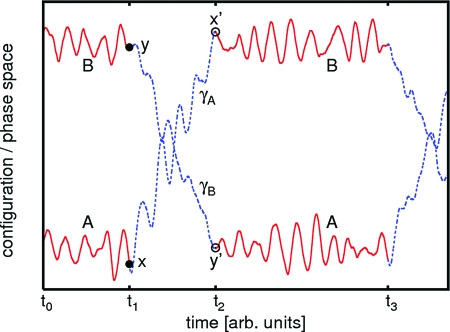
In the present paper, we develop a replica exchange method that uses nonequilibrium simulations to increase the overlap between replicas. Our approach, illustrated in Fig. 1, is summarized as follows. When attempting a swap between replicas A and B, we first perform a finite-time “work simulation” in replica A, during which we drag the system toward the region of phase space characteristic of equilibrium ensemble B, and vice-versa in replica B. We then attempt to swap the configurations thus generated by using a work-based acceptance criterion (Eq. 2). Although the system is driven away from equilibrium during the work simulations, the acceptance/rejection step ensures that detailed balance is preserved and that the replicas' equilibrium states are undisturbed. Although the CPU time devoted to the work simulations represents an added computational cost, the return on this investment is an increased acceptance probability. As a result, our method is able to achieve the same sampling efficiency as ordinary replica exchange but with fewer replicas.

Fig. 1.

Schematic depiction of RENS. The solid red lines depict intervals of equilibrium sampling in replicas A and B, and the dashed blue lines represent work simulations.

In Description of Method and Derivation, we describe and derive our method in detail, and then we illustrate it by using a model system adapted from ref. 3. We will use the acronym REM to refer to the usual replica exchange method, and RENS to denote our method based on nonequilibrium work simulations.

Description of Method

Let R₁,R₂,…R_M denote the collection of replicas, and let H _i(x) and T _i denote the Hamiltonian (energy function) and the temperature, respectively, of the canonical ensemble simulated in R_i. Here, x denotes a point in configuration space or phase space. Often, the H _i's are identical and only the temperatures differ, or vice-versa, but we need not assume this is the case. As in ref. 17, let us define a reduced Hamiltonian h _i(x) = H _i(x)/k _B T _i, so that the equilibrium distribution in R_i takes the form p _i ^eq ∝ exp(−h _i). When implementing REM, if 2 replicas R_A and R_B are found in configurations x and y at the time of an attempted swap, then the swap x ↔ y is accepted with probability P _acc = min{1,e ^−Δh}, where

If there is little overlap between the distributions p _A ^eq and p _B ^eq, then typically P _acc ≪ 1, and the swap is most likely rejected.

Fig. 1 illustrates RENS, the method we propose as an alternative. The time interval from t ₀ to t ₁ corresponds to independent, equilibrium sampling in each of the M replicas (two of which are depicted), using the reduced Hamiltonians h ₁,…h _M. At time t ₁, we decide to attempt a swap between replicas A and B. In lieu of an instantaneous exchange x ↔ y, we first perform a pair of work simulations. In R_A, the system evolves from time t ₁ to t ₂, as the reduced Hamiltonian is parametrically “switched” from h _A to h _B (Eq. 3.1). Let x′ denote the configuration at the end of this switching process, and w _A the reduced work performed on the system (Eq. 4.1). In R_B, we simulate the reverse process, parametrically switching from h _B to h _A, and define y′ and w _B analogously. We then attempt a swap between the 2 replicas, with acceptance probability

where w = w _A + w _B. If accepted, the configuration y′ is copied into replica A, and x′ into replica B, whereas, if rejected, the configurations revert to x and y. Subsequently, equilibrium sampling continues in R_A and R_B (using h _A and h _B, respectively) and in all other replicas until the next attempted swap. Fig. 1 depicts a successful replica swap at time t ₂ (open circles); if the attempt had been rejected, the replicas would have been reset to the states x, y, depicted as filled circles. Note that while work simulations are performed in R_A and R_B, the remaining replicas continue to sample at fixed h _i.

Thus, each replica alternates between sampling intervals at fixed h _i (Fig. 1, solid red lines), and work intervals (dashed blue lines). We next show that RENS satisfies detailed balance, in the following sense: In each replica R_i, if we discard the data generated during the work intervals and stitch together the remaining sampling intervals, we obtain a long trajectory that samples the distribution p _i ^eq. In effect, the acceptance criterion compensates for the fact that the system is driven out of equilibrium during the work simulations.

Our method is quite general and ultimately traces its validity to Crooks' extension of detailed balance to nonequilibrium trajectories (18). In a given implementation, however, the definition of reduced work depends on the dynamics chosen to model the evolution of the system. For discrete-time Monte Carlo dynamics, RENS is equivalent to the annealed swapping method of ref. 19 and closely related to the C-walking algorithm of ref. 20. In the following section, we derive our method for deterministic, reversible molecular dynamics (MD), and in the SI Appendix we extend this derivation to include stochastic evolution.

Derivation

For a pair of replicas R_A and R_B, we introduce a parametrized Hamiltonian h(x;λ) that interpolates from h(x;0) = h _A(x) to h(x;1) = h _B(x). To implement an attempted swap between these replicas, we first specify a switching protocol λ_t ^A, with λ₀ ^A = 0 and λ_τ ^A = 1. In R_A, starting from state x ₀ = x, we generate a trajectory γ_A during which the system evolves under the specified dynamics as the parameter λ is varied from 0 to 1 according to the switching protocol.

Simultaneously, in R_B we generate a trajectory γ_B, varying λ from 1 to 0 using the time-reversed protocol, λ_t ^B = λ_τ−t ^A,

The arrows denote the direction of time. The 2 trajectories γ_A and γ_B are illustrated by the dashed blue segments between times t ₁ and t ₂ in Fig. 1. We assume these trajectories are generated by deterministic equations of motion that are symmetric under time-reversal; for any trajectory γ_A = (x ₀ → x _τ) that evolves under the protocol λ_t ^A, the time-reversed trajectory ${\bar{\gamma }}_B=({\bar{x}}_0\leftarrow {\bar{x}}_{\tau })$ evolves under λ_t ^B, where $\bar{x}$ denotes inversion of momenta, p → −p. This assumption is satisfied by Hamiltonian dynamics, Nos–Hoover dynamics, and other equations of motion, provided the Hamiltonian itself is time-reversal symmetric, i.e. $h(x;\lambda )=h(\bar{x};\lambda )$.

For the trajectories γ_A and γ_B, we define the reduced work as follows:

Here, J _A = |∂x _τ/∂x ₀| and J _B = |∂y _τ/∂y ₀| are the Jacobians associated with propagating the system from the initial to the final point. Eq. 4 is analogous to the first law of thermodynamics, with lnJ representing a heat term associated with increase of system entropy.

When both work simulations have been completed, we attempt to swap the final configurations, assigning x′ = x _τ to replica B and y′ = y _τ to replica A. Schematically,

where the parallel arrows indicate the work simulations and the crossed arrows the attempted swap. The acceptance probability for the swap is given by Eq. 2. If it is rejected, the replicas are reset to their initial states, x = x ₀ and y = y ₀.

To analyze our method, it is useful to think of an expanded phase space containing 2 copies of the system, corresponding to R_A and R_B. In this space, we wish to sample the distribution p _AB ^eq(x,y) ∝ e ^{−h_A(x)−h_B(y)}. The work simulations, followed by the attempted swap, represent an elaborate trial Monte Carlo move (x, y) → (y′, x′) (21). Let P(y′,x′|x,y) be the corresponding transition probability—that is, the probability that the work simulations end in configurations x′ and y′, and the swap is accepted, given initial configurations x and y. To establish detailed balance, we must show that the net probability to observe a transition (x, y) → (y′, x′) is equal to that of the reverse transition $(\bar{x},\bar{y})\leftarrow (\bar{y}\text{'},\bar{x}\text{'})$ (3, 22), i.e. that

We will establish this result by introducing a few useful definitions and identities, which are then combined in Eq. 12.

For the work simulations in R_A and R_B, we can treat the final microstate as a function of the initial microstate (23),

obtained by integrating the deterministic equations of motion. We will use the notation

to denote the probability to arrive at x′ during a work simulation in R_A, starting from x; and similarly

Moreover, let

denote the joint probability for both events, and let

be the probability to accept the corresponding swap (Eq. 2). The transition probability P(y′,x′|x,y) is then given by the product P = πα.

The functions M _A and M _B introduced in Eq. 6 are related by our assumption of time-reversal symmetry. Namely, if x′ = M _A(x), then $\bar{x}=M_B(\bar{x}\text{'})$, which in turn implies

(Identifying q = lnJ as reduced heat, this result is equivalent to equation 9 of ref. 18.) Finally, the reduced work (Eq. 4) is odd under time-reversal,

Now, combining Eqs. 4 and 8 –11, we get

Because Eq. 12 is equivalent to Eq. 5, our scheme for generating configuration swaps preserves equilibrium in each replica.

Illustrative Dynamics

A simple dynamical scheme nicely illustrates our method. We suppose R_A and R_B are described by different temperatures, T _A < T _B, but the same H, and we construct Hamilton's equations augmented by a term proportional to $\stackrel{.}{\lambda }$ :

with s _λ = (1/2T _λ)(dT _λ/dλ). Here, T _λ interpolates from T ₀ = T _A to T ₁ = T _B. The extra term in Eq. 13 provides rudimentary temperature control during the work simulations. As λ is varied from 0 to 1 in replica A, the momenta are scaled up, effectively heating up the system; in replica B, the system is cooled. An equivalent rescaling of momenta is standard practice in REM, where it is performed instantaneously rather than over the course of a trajectory; see equation 12 of ref. 24.

These dynamics do not preserve phase space volume ∇ · $\stackrel{.}{x}=N\stackrel{.}{\lambda }{s}_{\lambda }$ ≠ 0, where N is the number of degrees of freedom. The Jacobian for a work simulation in R_A is then

and in R_B we have J _B = J _A ⁻¹. (The fact that J _A and J _B do not depend on initial conditions is specific to these dynamics.)

By heating the system during the work simulation in R_A and cooling it in R_B, the scaling term $\stackrel{.}{\lambda }{s}_{\lambda }$ p _i increases the probability for accepting the configuration swap. (Indeed, for a system of ideal gas particles, evolution under Eq. 13 exactly transforms a Maxwell–Boltzmann distribution from temperature T _A to T _B, or vice versa. In this special case, w _A + w _B = 0, and P _acc = 1.)

Even when RENS is used with stochastic equations of motion, such as Langevin dynamics or the Andersen thermostat (see SI Appendix), it is useful to include the scaling term in Eq. 13, as this term dynamically adjusts the momenta in response to the changing temperature T _λ.

Efficiency Considerations and Numerical Results

While our method is valid for arbitrary choice of switching time, τ, it is instructive to consider two limiting cases. In the sudden limit, τ = 0, we have w = Δh (Eqs. 1, 3, 4), as noted by Wyczalkowski and Pappu (25).† In this case, RENS reduces to REM, and if there is little overlap between p _A ^eq and p _B ^eq, then P _acc ≪ 1. For a properly thermalized system in the opposite quasi-static limit, τ → ∞, the system evolves reversibly as λ is varied infinitely slowly; the reduced work is the corresponding reduced free energy difference,

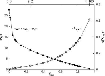
where $f_i=-ln\int dx{e}^{-h_i}$; hence w = 0 and P _acc = 1 (Eq. 2). Thus we can manipulate the acceptance probability P _acc by adjusting the switching time τ. Generically, we expect that the more slowly we perform the work simulation, the greater the probability to accept the configuration swap (see Fig. 4). This expectation implies a computational tradeoff—what is the optimal value of τ?—which we now address with a simple analysis.

Fig. 4.

Average reduced work (filled circles) and observed acceptance frequency (open circles) as functions of the fraction of simulation time devoted to work intervals. 〈P _acc〉 is defined as the fraction of attempted replica exchanges that were accepted in a given test run. At f _sw = 0, corresponding to ordinary (instantaneous) replica exchange, 〈P _acc〉≈ 0.003.

We consider M replicas and assume for specificity that we are mainly interested in sampling from one of them, which we denote as the primary replica; the remaining replicas serve only to enhance sampling in the primary replica. (A similar analysis can be carried out if we are equally interested in sampling all M ensembles.) The term output trajectory will denote the trajectory obtained by concatenating the sampling intervals generated in the primary replica after discarding the work intervals. We let ${\bar{\tau }}_{\text{eq}}$ denote the average duration of a sampling interval. The output trajectory samples the equilibrium distribution of interest and is in effect the end product of our method. Let t _c denote a characteristic correlation time associated with this output trajectory, and define

In terms of these quantities, the sample cost

is a measure of the total computational cost, summed over all M replicas (26), of producing a single, statistically independent sample in the primary replica. The factor (1 + X) accounts for the overhead cost of the work intervals: For every unit of sampling time, X units of time were devoted to the discarded work simulations. The sample cost provides a figure of merit; the smaller the value of t*, the more efficiently we are using the computational resources. While the correlation time t _c generally decreases with increasing M or τ —through the randomizing effect of successful replica exchanges—in Eq. 17 this trend competes with the overhead factors M and 1 + X.

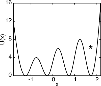
To investigate these issues, we simulated a model system of n _p = 10 particles, moving independently in the potential shown in Fig. 2. We took M = 2 replicas, at T _A = 0.30 and T _B = 2.0 (arbitrary units). In the primary replica at T _A = 0.30, sampling is hindered by the barriers separating the local minima of U(x); whereas at T _B = 2.0 the particles are able to jump from well to well. We performed MD simulations by using Eq. 13 in combination with an Andersen thermostat (27) (see SI Appendix).

Fig. 2.

Mock-up of a rough potential energy landscape adapted from ref. 3, Chapter 14. An asterisk marks the fourth well (x ≥ 1.25). Ordinary replica exchange works well for 1 particle, but encounters difficulties when n _p = 10.

While REM performs well for a single particle in this potential (3), when n _p = 10 it encounters difficulties due to poor phase space overlap, as can be understood using an argument of Kofke's (28). Typically, in R_A each particle is found near a local minimum of U(x), whereas in R_B they are distributed more uniformly. Thus a configuration swap is likely to be accepted only if all particles in R_B are found very near to the minima of U(x), which is unlikely when n _p ≫ 1. With RENS, the work simulation in R_B increases the swap acceptability by shepherding the particles closer to the minima of U(x).

When simulating this system using RENS, the replicas “toggle” between sampling and work intervals (Fig. 1). We implemented this as follows. During an interval of sampling, a work simulation was initiated at random, with an attempt rate r = 0.166. Once initiated, the work interval lasted for the prescribed switching time τ, after which the replicas reverted to sampling, and so on. Thus the average duration of a sampling interval was ${\bar{\tau }}_{\text{eq}}=1/r\approx 6.0$, which is roughly 3 times the relaxation rate within one of the local wells of U.

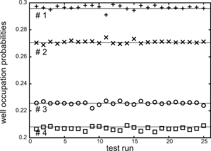
With these parameters, we performed 25 test runs, with τ ranging from 0 to 100. To establish proof of principle, we tabulated empirical occupation probabilities for the 4 wells by following a tagged particle in the output trajectory. For each test run, we found that the relative amount of time the particle spent in each well was in agreement with the equilibrium distribution, within statistical error (Fig. 3).

Fig. 3.

Observed occupations of wells 1–4, obtained by following a single tagged particle in the output trajectory, for each of the 25 test runs. The solid horizontal lines are exact values determined by integration of the single-particle Boltzmann distribution.

For the same set of test runs, in Fig. 4 we plot the observed swap acceptance frequency and average reduced work as functions of the fraction of simulation time devoted to the work intervals,

As anticipated, with increasing f _sw (or τ ) we approach the reversible limit of w = 0 and P _acc = 1 (Eq. 15).

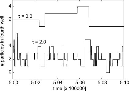
To illustrate the accelerated sampling achieved with our method, we considered n ₄(t), the number of particles found in the fourth well of U(x) at time t of the output trajectory. Fig. 5 shows n ₄(t) for segments of the τ = 0.0 and τ = 2.0 test runs. For the relatively modest cost of setting aside 25% of the simulation time to the work intervals, transitions into and out of the fourth well are greatly facilitated.

Fig. 5.

n ₄(t) is plotted over an interval of time for output trajectories obtained with REM (upper trace, shifted for clarity) and RENS (lower trace). The 2 traces represent roughly the same number of attempted replica exchanges (≈ 1700) but reveal substantially different acceptance rates.

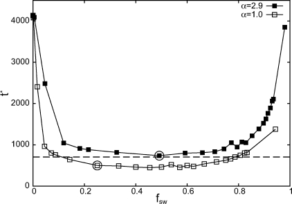
Next, for each test run we used block-averaging (29) to evaluate a correlation time $t_c=(1/{\sigma }^2){\int }_{-\infty }^{+\infty }dtc(t)$, where σ² and c(t) are the variance and autocorrelation of n ₄(t). In Fig. 6, we plot the sample cost t* for each test run (empty squares). At f _sw = 0 (that is, when using REM), this cost is high, t* > 4,000; few swaps are accepted, and particles are trapped in the fourth well for long times. As we increase f _sw, the sample cost drops significantly, reaching a broad minimum t* ∼ 450 − 500 for f _sw ∼ 0.2 − 0.6; here the allocation of CPU time to work intervals delivers a clear benefit. For f _sw > 0.6, we enter a regime of diminishing returns: 〈P _acc〉 continues to increase with τ (Fig. 4), but not enough to justify the expense of increasingly long work simulations.

Fig. 6.

Sample cost t* plotted against f _sw both with and without adjustment for increased relative cost of work simulations (see Efficiency Considerations and Numerical Results). The circles identify the run at τ = 2.0. The dashed line is the sample cost of REM with M = 4 replicas.

To this point, we have neglected the computational cost of the “acceptance/rejection” step itself, as well as that of the possible subsequent exchange of configurations (which typically involves communication between different processors). Moreover, we have assumed identical costs, per unit simulation time, for the work and the sampling intervals. It is easy enough to drop the latter assumption: We replace X by αX in Eqs. 17 and 18, where α is the observed CPU cost of generating a work simulation relative to that of a sampling trajectory of equal duration. In our test runs, we found α = 2.9, and the points shown as filled squares in Fig. 6 have been adjusted for this value. (If our model had included particle–particle interactions, α would have been closer to unity.)

Whether or not we make the adjustment to account for α≠1, Fig. 6 clearly shows that for a fixed set of replicas, it can be highly advantageous to use nonequilibrium work simulations to generate attempted configuration swaps. The benefits of increased acceptance substantially outweigh the overhead cost of generating the trial configurations.

With RENS, we improve efficiency by tuning the switching time, τ, as in Fig. 6. With REM, one can instead vary the number of replicas. To compare these 2 options, we performed test runs of REM (τ = 0) at M = 2,3,…11. (In each run, we set T ₁ = 0.30 and T _M = 2.0, with intermediate replicas spaced evenly in T ⁻¹.) Among these runs, the smallest sample cost, t* = 706, was achieved with M = 4 replicas, and is shown as a straight line in Fig. 6. This value is comparable to the optimal sample cost achieved with RENS using M = 2. Thus for this simple system, RENS is able to match the efficiency of REM with fewer replicas.

Discussion

When applying REM to a problem of interest, the phase space overlap requirement dictates a minimum number of replicas, M*, needed to achieve a reasonable swap acceptance frequency. With RENS, the work simulations have the effect of increasing phase space overlap, thus allowing for fewer replicas, M < M*. There are several reasons why one might wish to exploit this flexibility.

1. Most obviously, if we perform simulations using a cluster of P processors, then RENS allows us to assign 1 replica per processor—the easiest and most natural (and traditional) allocation—even if P < M*.

2. It is often useful to picture replica exchange as a diffusion process in which trajectories hop randomly along the chain R₁,…,R_M. In this picture, ∼ M ² successful swaps are needed for a given trajectory to accomplish an entire transit between R₁ to R_M. Thus using fewer replicas (with RENS) can significantly reduce the cost of interprocessor communication associated with attempted configuration swaps.

3. REM is often implemented synchronously: Swaps are attempted only after every replica completes a predetermined duration of equilibrium sampling. With 1 replica per processor, this can be highly inefficient, limited by the speed of the slowest processor. RENS lends itself naturally to asynchronous implementation. A master process initiates work simulations in a randomly chosen replica pair, whereas the remaining replicas, unaffected, continue sampling.

4. With any replica exchange strategy, there are parameters we adjust to optimize efficiency, such as the number of replicas, M, and the choice of intermediate temperatures or Hamiltonians. It is potentially very useful to improve efficiency adaptively, during the actual production run (30). RENS offers a relatively painless way to accomplish this, namely by adjusting the durations of the work simulations. For example, if it is observed that a low P _acc between R_n and R_i+1 poses a bottleneck for efficient sampling, then the switching time for that replica pair, τ_n,n+1, can be increased.

5. To this point, we have treated the data generated during the work simulations as “junk” to be discarded after the attempted configuration swap. However, by a trick of statistical reweighting one can scavenge equilibrium information from such nonequilibrium trajectories (see equation 4 of ref. 31). The work simulations themselves can then contribute to the equilibrium sampling in each replica, thus increasing the efficiency of RENS. For Monte Carlo sampling, Frenkel (32) has developed an analogous, thrifty algorithm that relies on the “waste-recycling” of otherwise rejected trial moves.

These considerations suggest that RENS offers a flexible, efficient and useful sampling strategy. We expect that it can further be enhanced through combination with other approaches such as solute tempering (7) and generalized effective potentials (11), or by the use of large time steps (33) or artificial flow fields (34) during the work simulations.

The simple model we have borrowed (3) is well suited as an initial test case of our method: It exhibits the difficulties faced by REM for large (n _p = 10) systems, its equilibrium properties can be evaluated exactly (Fig. 3), and its efficiency can be computed with high statistical accuracy for many values of τ (Fig. 6). Further assessments of our method will come both from applications to problems of genuine physical interest and from analytical and semianalytical treatments that have provided useful insight into the performance of replica exchange strategies (17, 28, 30, 35–37).

References

- 1.Swendsen RH, Wang JS. Replica Monte-Carlo simulation of spin-glasses. Phys Rev Lett. 1986;57:2607–2609. doi: 10.1103/PhysRevLett.57.2607. [DOI] [PubMed] [Google Scholar]
- 2.Earl DJ, Deem MW. Parallel tempering: Theory, applications, and new perspectives. Phys Chem Chem Phys. 2005;7:3910–3916. doi: 10.1039/b509983h. [DOI] [PubMed] [Google Scholar]
- 3.Frenkel D, Smit B. Understanding Mol Simul. San Diego: Academic; 2002. [Google Scholar]
- 4.Hukushima K, Nemoto K. Exchange Monte Carlo method and application to spin glass simulations. J Phys Soc Jpn. 1996;65:1604–1608. [Google Scholar]
- 5.Gnanakaran S, Nymeyer H, Portman J, Sanbonmatsu KY, Garcia AE. Peptide folding simulations. Curr Opin Struc Biol. 2003;13:168–174. doi: 10.1016/s0959-440x(03)00040-x. [DOI] [PubMed] [Google Scholar]
- 6.Fukunishi H, Watanabe O, Takada S. On the Hamiltonian replica exchange method for efficient sampling of biomolecular systems: Application to protein structure prediction. J Chem Phys. 2002;116:9058–9067. [Google Scholar]
- 7.Liu P, Kim B, Friesner RA, Berne BJ. Replica exchange with solute tempering: A method for sampling biological systems in explicit water. Proc Natl Acad Sci USA. 2005;102:13749–13754. doi: 10.1073/pnas.0506346102. [DOI] [PMC free article] [PubMed] [Google Scholar]
- 8.Liu P, Huang X, Zhou R, Berne BJ. Hydrophobic aided replica exchange: An efficient algorithm for protein folding in explicit solvent. J Phys Chem B. 2006;38:19018–19022. doi: 10.1021/jp060365r. [DOI] [PMC free article] [PubMed] [Google Scholar]
- 9.Hansmann UHE. Parallel tempering algorithm for conformational studies of biological molecules. Chem Phys Lett. 1997;281:140–150. [Google Scholar]
- 10.Whitfield TW, Bu L, Straub JE. Generalized parallel sampling. Physica A. 2002;305:157–171. [Google Scholar]
- 11.Jang S, Shin S, Pak Y. Replica-exchange method using the generalized effective potential. Phys Rev Lett. 2003;91:058305. doi: 10.1103/PhysRevLett.91.058305. [DOI] [PubMed] [Google Scholar]
- 12.Calvo F, Doye JPK. Entropic tempering: A method for overcoming quasiergodicity in simulation. Phys Rev E. 2000;63:010902. [Google Scholar]
- 13.Faller R, Yan Q, de Pablo JJ. Multicanonical parallel tempering. J Chem Phys. 2002;116:5419–5423. [Google Scholar]
- 14.Mitsutake A, Sugita Y, Okamoto Y. Generalized-ensemble algorithms for mol simuls of biopolymers. Biopolymers. 2001;60:96–123. doi: 10.1002/1097-0282(2001)60:2<96::AID-BIP1007>3.0.CO;2-F. [DOI] [PubMed] [Google Scholar]
- 15.Fenwick MK, Escobedo FA. Expanded ensemble and replica exchange methods for simulation of protein-like systems. J Chem Phys. 2003;119:11998–12010. [Google Scholar]
- 16.Rick SW. Replica exchange with dynamical scaling. J Chem Phys. 2007;16:054102. doi: 10.1063/1.2431807. [DOI] [PubMed] [Google Scholar]
- 17.Park S. Comparison of the serial and parallel algorithms of generalized ensemble simulations: An analytical approach. Phys Rev E. 2008;77:016709. doi: 10.1103/PhysRevE.77.016709. [DOI] [PubMed] [Google Scholar]
- 18.Crooks GE. Nonequilibrium measurements of free energy differences for microscopically reversible Markovian systems. J Stat Phys. 1998;90:1481–1487. [Google Scholar]
- 19.Opps S, Schofield J. Extended state-space Monte Carlo methods. Phys Rev E. 2001;63:056701. doi: 10.1103/PhysRevE.63.056701. [DOI] [PubMed] [Google Scholar]
- 20.Brown S, Head-Gordon T. Cool-walking: A new Markov chain Monte Carlo sampling method. J Comput Chem. 2003;24:68–76. doi: 10.1002/jcc.10181. [DOI] [PubMed] [Google Scholar]
- 21.Stern H. A molecular simulation with variable protonation states at constant pH. J Chem Phys. 2007;126:164112. doi: 10.1063/1.2731781. [DOI] [PubMed] [Google Scholar]
- 22.Chandler D. Introduction to Modern Statistical Mechanics. New York: Wiley; 1987. [Google Scholar]
- 23.Oberhofer H, Dellago C, Geissler PL. Biased sampling of nonequilibrium trajectories: Can fast switching simulations outperform conventional free energy calculation methods? J Phys Chem B. 2005;109:6902–6915. doi: 10.1021/jp044556a. [DOI] [PubMed] [Google Scholar]
- 24.Sugita Y, Okamoto Y. Replica-exchange molecular dynamics method for protein folding. Chem Phys Lett. 1999;314:141–151. [Google Scholar]
- 25.Wyczalkowski MA, Pappu RV. Satisfying the fluctuation theorem in free-energy calculations with Hamiltonian replica exchange. Phys Rev E. 2008;77:026104. doi: 10.1103/PhysRevE.77.026104. [DOI] [PubMed] [Google Scholar]
- 26.Zuckerman DM, Lyman E. A second look at canonical sampling of biomolecules using replica exchange simulation. J Chem Theory Comput. 2006;2:1200–1202. doi: 10.1021/ct600297q. [DOI] [PubMed] [Google Scholar]
- 27.Andersen HC. Molecular dynamics simulations at constant pressure and/or temperature. J Chem Phys. 1980;72:2384–2393. [Google Scholar]
- 28.Kofke DA. On the acceptance probability of replica-exchange Monte Carlo trials. J Chem Phys. 2002;117:6911–6914. [Google Scholar]
- 29.Flyvbjerg H, Petersen HG. Error estimates on averages of correlated data. J Chem Phys. 1989;91:461–466. [Google Scholar]
- 30.Trebst S, Troyer M, Hansmann UHE. Optimized parallel tempering simulations of proteins. J Chem Phys. 2006;124:174903. doi: 10.1063/1.2186639. [DOI] [PubMed] [Google Scholar]
- 31.Hummer G, Szabo A. Free energy reconstruction from nonequilibrium single-molecule pulling experiments. Proc Natl Acad Sci USA. 2001;98:3658–3661. doi: 10.1073/pnas.071034098. [DOI] [PMC free article] [PubMed] [Google Scholar]
- 32.Frenkel D. Speed-up of Monte Carlo simulations by sampling of rejected states. Proc Natl Acad Sci USA. 2004;101:17571–17575. doi: 10.1073/pnas.0407950101. [DOI] [PMC free article] [PubMed] [Google Scholar]
- 33.Lechner W, Oberhofer H, Dellago C, Geissler PL. Equilibrium free energies from fast-switching trajectoies with large time steps. J Chem Phys. 2006;124:044113. doi: 10.1063/1.2162874. [DOI] [PubMed] [Google Scholar]
- 34.Vaikuntanathan S, Jarzynski C. Escorted free energy simulations: Improving convergence by reducing dissipation. Phys Rev Lett. 2008;100:190601. doi: 10.1103/PhysRevLett.100.190601. [DOI] [PubMed] [Google Scholar]
- 35.Zheng W, Andrec M, Gallicchio E, Levy RM. Simulating replica exchange simulation of protein folding with a kinetic network model. Proc Natl Acad Sci USA. 2007;104:15340–15345. doi: 10.1073/pnas.0704418104. [DOI] [PMC free article] [PubMed] [Google Scholar]
- 36.Sindhikara D, Meng Y, Roitberg AE. Exchange frequency in replica exchange molecular dynamics. J Chem Phys. 2008;128:024103. doi: 10.1063/1.2816560. [DOI] [PubMed] [Google Scholar]
- 37.Nymeyer H. How efficient is replica exchange molecular dynamics? An analytic approach. J Chem Theory Comput. 2008;4:626–636. doi: 10.1021/ct7003337. [DOI] [PubMed] [Google Scholar]
Associated Data
This section collects any data citations, data availability statements, or supplementary materials included in this article.