Abstract
Recent advances in high-throughput genotyping have inspired increasing research interests in genome-wide association study for diseases. To understand underlying biological mechanisms of many diseases, we need to consider simultaneously the genetic effects across multiple loci. The large number of SNPs often makes multilocus association study very computationally challenging because it needs to explicitly enumerate all possible SNP combinations at the genome-wide scale. Moreover, with the large number of SNPs correlated, permutation procedure is often needed for properly controlling family-wise error rates. This makes the problem even more computationally demanding, since the test procedure needs to be repeated for each permuted data. In this paper, we present FastChi, an exhaustive yet efficient algorithm for genome-wide two-locus chi-square test. FastChi utilizes an upper bound of the two-locus chi-square test, which can be expressed as the sum of two terms – both are efficient to compute: the first term is based on the single-locus chi-square test for the given phenotype; and the second term only depends on the genotypes and is independent of the phenotype. This upper bound enables the algorithm to only perform the two-locus chi-square test on a small number of candidate SNP pairs without the risk of missing any significant ones. Since the second part of the upper bound only needs to be precomputed once and stored for subsequence uses, the advantage is more prominent in large permutation tests. Extensive experimental results demonstrate that our method is an order of magnitude faster than the brute force alternative.
1. Introduction
Disease association study analyzes genetic variation across a population consisting of diseased and healthy individuals. The most abundant source of genetic variation in mammalian genome is represented by single nucleotide polymorphisms (SNPs), which account for heritable inter-individual differences in complex phenotypes. The allele differences at these single base sites are usually represented as binary variables (e.g. inbred mice) or ternary variables (e.g. human subjects). Recent advancement of the technologies that enable genotyping a vast number of genetic polymorphism has made genome wide association study possible. Initial reports on genome-wide searching for disease associated genes are appearing in the literature 6,10,15.
Most existing analytical methods consider each genetic marker individually 20. In many cases, however, the diseases are complex traits, that is, they are likely due to the interactions among multiple genes 2,17. In order to understand their underlying biological mechanisms, we need to consider simultaneously the joint effects of genotypes across multiple loci. Various machine learning models have been adopted to study the interactions among genes, such as neural networks 3,18 and classification and regression trees (CART)12,22. Under the assumption that the number of SNPs is small, exhaustive algorithms that explicitly enumerate all possible SNP combinations have been developed 7,13. Since these methods explicitly enumerate all possible SNP combinations, they are not suitable for genome-wide association studies.
The number of SNPs in public datasets ranges from thousands to hundreds of thousands1,21. The computational burden of searching for interactions among the large number of SNPs often makes the complete genome wide association study intractable. SNP tagging 5,16 have been widely used to reduce the number of SNPs to be analyzed. The goal of SNP tagging is to select a subset of SNPs that can be used as proxies for all SNPs in the genome. The tagged SNPs are then used in the association study. These methods are not complete because some important SNPs may not be tagged.
The computational challenge of genome-wide association study is also caused by another problem known as multiple testing problem. It can be described as the potential increase in Type I error when statistical tests are performed multiple times. Let α be the significant level for each independent test. If n independent comparisons are performed, the family-wise error α′ is given by α′ = 1 − (1 − α)n. For example, if α = 0.05 and we test twenty null hypotheses, then we have probability α′ = 1 − 0.9520 = 0.64 to get at least one spurious result. Permutation testing has been the gold standard for assessing significance levels in association studies using multiple markers. However, it is time consuming since the test procedure needs to be repeated for every permutation. To make this process feasible, other correction methods have been proposed 8,9. Some recent work 23 addresses the problem of two-locus quantitative phenotype association mapping when large permutation tests are needed. However, this method focuses on the case where the phenotypes are continuous variables, hence is not readily applicable to case-control study of diseases.
Theoretically well studied, the chi-square test has been widely used in association studies 11. In this paper, we examine the computational aspect of the chi-square test. We present an efficient algorithm, FastChi, and show that the standard chi-square test can be applied in the genome-wide scale for two-locus association study even when large permutation tests are performed. Different from the algorithms applying heuristics, tagging SNPs, or adopting other correction methods, FastChi is an exhaustive algorithm. It guarantees to find the optimal solution. Yet, FastChi does not need to explicitly compute the chi-square value for every SNP pair. It utilizes an upper bound of the two-locus chi-square test value, which is the sum of two terms: one based on the single-locus chi-square test, and the other based on the pair-wise SNP genotypes. Using this bound, a large portion of the SNP-pairs are pruned without performing the tests. Due to space limitation, in this paper, we mainly focus on the case where the SNPs are binary variables which are encoded using {0, 1}. We also have similar results for the case where the SNPs are ternary variables, which will be discussed in Section 5.
2. Problem Definition
Let {X1, X2, ⋯, XN} be the set of all biallelic SNPs , and Y be the binary phenotype of interest (e.g., disease or non-disease). For any SNP Xi (1 ≤ i ≤ N), we represent its chi-square test value with Y as χ2(Xi, Y ). For any SNP-pair Xi and Xj, the chi-square test value is denoted as χ2(XiXj, Y ). We formalize the problem as follows. Given the set of N SNPs and a phenotype Y for a set of M individuals, let Y′ = {Y1, Y2, ⋯ YK} be the set of K permutations of Y. There are two possible cases:
(1) For a single pass association study, i.e., no permutation correction needed: find all SNP-pairs (XiXj) such that χ2(XiXj, Y) ≥ θ.
(2) If there are multiple phenotype permutations: for each Yk ∈ Y′, find all SNP-pairs (XiXj) such that χ2(XiXj, Yk) ≥ θ,(1 ≤ k ≤ K).
Our problem formalization can also be applied in other problem settings. For example, it is easy to modify this problem definition to find the top-k SNP-pairs that have the largest chi-square test values among all SNP-pairs. In this scenario, θ would be a dynamic value, i.e., the k-th largest chi-square test value identified by the algorithm so far.
3. The FastChi Algorithm
We first present the upper bound of the two-locus chi-square test value in Section 3.1. Then we show how our algorithm FastChi utilizes the upper bound to achieve efficient two-locus chi-square testing. In Section 3.2, we describe the method for a single phenotype Y. In Section 3.3, we discuss how FastChi performs under permutation procedure.
3.1. The Upper Bound
Let A, B, C, D represent the following events respectively: Y = 0 ⋀ Xi = 0; Y = 0 ⋀ Xi = 1; Y = 1 ⋀ Xi = 0; Y = 1 ⋀ Xi = 1. Let Eevent and Oevent denote the expected value and observed value of an event. T1, T2, S1, S2,ℛ1, and ℛ2 represent the formulas shown in Table 1. We have the upper bound of χ2(XiXj, Y ) stated in Theorem 3.1. The derivation of the upper bound is omitted due to space limitation.
Table 1.
Notations used in the upper bound
| Symbols | Formulas |
|---|---|
| T 1 | |
| S 1 | |
| ℛ 1 | |
| T 2 | |
| S 2 | |
| ℛ 2 |
Theorem 3.1.
(Upper bound of χ2(XiXj, Y))
3.2. A Single Phenotype
It is obvious that, if the upper bound of χ2(XiXj, Y ) is less than θ, there is no need to calculate the exact value of χ2(XiXj, Y), which is guaranteed to be smaller than θ. We now discuss this idea in further detail.
For every Xi (1 ≤ i ≤ N), let AP (Xi) = {(XiXj)|i+1 ≤ j ≤ N} be the SNP-pairs with Xi being the SNP of lower index value. For all SNP-pairs in AP (Xi), the phenotype Y and SNP Xi do not vary, thus OA, OB, OC and OD are constants for all SNP-pairs in AP(Xi). The number of individuals, M, is also a constant. Thus, in the upper bound, T1S1 and T2S2 are constants. Moreover, χ2(Xi, Y ) is a constant for a given Xi, and θ is given too. Therefore, ℛ1 and ℛ2 are the only variables that depend on Xj and may vary for different SNP-pairs (XiXj)∈ AP(Xi). Thus for a given Xi, we can treat equation χ2(Xi, Y) + T1S1ℛ2 + T2S2ℛ2 = θ as a straight line in the 2-D space of ℛ1 and ℛ2.
From now on, we use ℛ1(XiXj) and ℛ2(XiXj) to represent the specific values of ℛ1 and ℛ2 for the SNP-pair (XiXj). The following proposition specifies the values that ℛ1(XiXj) and ℛ2(XiXj) can take.
Proposition 3.1
If there are m 0's and (M – m) 1's in Xi, then for any (XiXj) ∈ AP(Xi), the possible values that ℛ1(XiXj) can take are: . The possible values that ℛ2(XiXj) can take are: .
Therefore, for all (XiXj) ∊ AP (Xi), in the 2-D space of ℛ1 and ℛ2, (ℛ1(XiXj),ℛ2(XiXj)) falls in the region [0, 1]×[0, 1]. The line χ2(Xi, Y )+ T1S1ℛ1 + T2S2ℛ2 = θ divides this region into two parts: one above the line and one below it. Among the SNP-pairs in AP (Xi), we only need to perform the test for those ones whose (ℛ1(XiXj), ℛ2(XiXj)) values are above the line, i.e., whose upper bounds are greater than the threshold θ. We refer to such SNP-pairs as candidate SNP-pairs.
Example 3.1
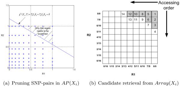
Suppose that there are 32 individuals, half alleles of Xi are 0's, and half are 1's. Thus, for the SNP-pairs in AP (Xi), the possible values of ℛ1(XiXj) (and ℛ2(XiXj)) are . Figure 1(a) shows the 2-D space of ℛ1 and ℛ2. The blue stars represent the values that (ℛ1(XiXj),ℛ2(XiXj)) can take. The line χ2(Xi, Y) + T1S1ℛ1 + T2S2ℛ2 = θ is also plotted in the figure. The candidate SNP-pairs are those whose (ℛ1(XiXj),ℛ2(XiXj)) values are in the shaded region. The ones whose (ℛ1(XiXj),ℛ2(XiXj)) values fall below the line can be pruned without any further test.
Figure 1.
Applying the upper bound
To efficiently retrieve the candidates, SNP-pairs (XiXj) in AP(Xi) are grouped by their (ℛ1(XiXj),ℛ2(XiXj)) values and indexed in a 2D array, referred to as Array(Xi).
Example 3.2
Following Example 3.1, Figure 1(b) shows the 9 × 9 array, Array(Xi), whose entries represent the possible values of (ℛ1(XiXj),ℛ2(XiXj)) for SNP-pairs (XiXj) ∊ AP(Xi). The ℛ1(XiXj) (ℛ2(XiXj)) value of each column (row) is noted beneath (left to) each column (row). Each entry of the array is a pointer to the SNP-pairs having the corresponding (ℛ1(XiXj),ℛ2(XiXj)) values.
In order to find the candidates SNP-pairs whose upper bounds are greater than θ, we start from the right most column of the array, i.e., the entries having the largest ℛ1(XiXj) value. We scan this column from the top (entries with larger ℛ2(XiXj) values) towards the bottom (entries with smaller ℛ2(XiXj) values). If an entry satisfies the inequality χ2(Xi, Y )+T1S1ℛ1+T2S2ℛ2 ≥ θ, then the SNP-pairs indexed by it are the candidates subject to the chi-square tests. Once we reach an entry violating the inequality, we stop searching the current column, since the remaining entries in the column will not satisfy the inequality. We then move to the top entry of the column left to it and repeat the same scanning process. This whole process terminates when (1) we finish examining all columns or (2) we reach a column whose top entry does not satisfy the inequality.
Example 3.3
Continuing with Examples 3.1 and 3.2, the entries numbered from 1 to 14 in Figure 1(b) are the ones visited by the scanning process. The numbers show the order in which the entries are visited. Only the SNP-pairs indexed by shaded entries need to be evaluated by chi-square tests. The SNP-pairs indexed by the blank entries, including the entries on the boundary can be safely pruned.
3.3. Permuting the Phenotype
Let Y′ = {Y1, Y2, ⋯ , YK} be the K permutations of the phenotype Y. The upper bound in Theorem 3.1 can be easily incorporated in the algorithm to handle the permutations: For any (XiXj) ∊ AP (Xi), its (ℛ1(XiXj),ℛ2(XiXj)) value does not change over different permutations. That is, for every SNP Xi, the indexing structure Array(Xi) is independent of permutations in Y′. Thus, for each Xi, once we get Array(Xi), it can be reused in all permutations.
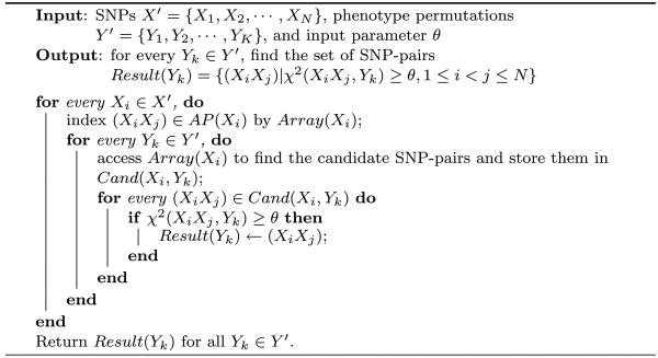
The FastChi algorithm is described in Algorithm 1. For each Xi, FastChi first indexes (XiXj) ∊ AP(Xi) using Array(Xi). Then it finds the set of candidate SNP-pairs Cand(Xi,Yk) by accessing Array(Xi) for every phenotype permutation Yk. The candidates in Cand(Xi,Yk) are then evaluated for their chi-square test values. The candidates whose chi-square test values are greater than or equal to θ are reported by the algorithm.
Algorithm 1.
FastChi1
Time complexity
The complexity to build the indexing structure for all SNPs is O(N2M). The worst case for accessing all Array(Xi) for all permutations is O(KNM2). Let C = σi,k |Cand(Xi,Yk)| be the total number of candidates. The time complexity of FastChi is O(N2M+KNM2+CM). Note that the time complexity of the brute force approach is O(KN2M). The number of SNPs N is the dominant factor here.
Space complexity
The dataset size is O((N + K)M). The size of the Array(Xi) is O(M2 + N). For each Xi, once the evaluation process is over for all permutations, Array(Xi) can be cleared from the memory. Therefore, the space complexity of FastChi is O((N + K)M) + O(M2 + N). Since M is usually much smaller than N, this space complexity is linear to the dataset size.
4. Experimental Results
We present extensive experimental results on evaluating the performance of FastChi. FastChi is implemented in C++. The experiments are performed on a 2.4 GHz PC with 1G memory running WindowsXP system.
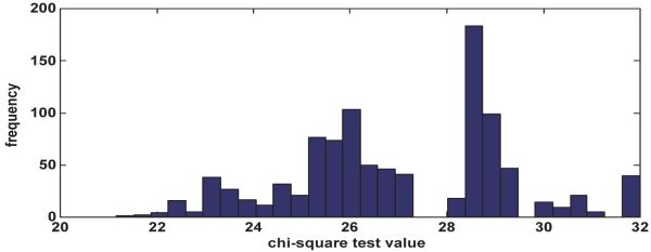
The SNP dataset used in the experiments is extracted from a set of combined SNPs from the 140k Broad/MIT mouse dataset 21 and 10k GNF 1 mouse dataset. This merged dataset has 156,525 SNPs for 71 mouse strains. The missing values in the dataset are imputed using NPUTE 14. The default setting of the experiments are as follows: the phenotypes are random permutations of binary variable with half 0's and half 1's, #individuals = 32, #SNPs=8k, #permutations=20. There are 60,970 unique SNPs for these 32 mice strains. To find the appropriate threshold value, we permute the phenotypes 1000 times. Figure 2 shows the distribution of the maximum chi-square test values of the 1000 permutations. Using a critical significance level of 1%, we set the default threshold value of θ to be 32.
Figure 2.
Distribution of the maximum chi-square test values
Note that these experimental settings are chosen to demonstrate the performance gain and enhanced scalability offered by FastChi over the brute force approach. In real utility, one may use larger SNP panels and/or more permutation tests. The performance of FastChi is expected to follow the same trends presented in the remainder of this section.
FastChi v.s. the brute force approach
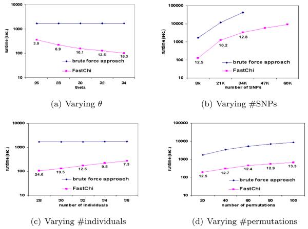
As far as we know, FastChi is the first algorithm addressing the problem of how to scale up the complete two-locus Chi-square test involving large permutation test. For comparison, we show the runtime of FastChi versus the runtime of the brute force approach. The implementation of the brute force approach includes the computation of two-locus chi-square test for every SNP pairs. Figures 3(a) to 3(d) show the running time comparison under various parameter settings. The numbers below the runtime line of FastChi indicate the ratio of the runtime of the brute force approach and the runtime of FastChi. Figure 3(a) shows that the runtime of FastChi dramatically decreases as θ increases. FastChi offers 3.9 fold speedup when θ = 26 and 16.3 fold speedup when θ = 34. Figure 3(b) shows that FastChi is an order of magnitude faster than the brute force approach. Figure 3(c) shows that the runtime of FastChi increases as the number of individuals increases. This is because more SNPs-pairs are expected to have larger chi-square values when the number of individuals increases. Their upper bounds will also increase accordingly. In practice, it is reasonable to set higher threshold values for the datasets containing more individuals. Figure 3(d) shows that FastChi is consistently an order of magnitude faster than the brute force approach in permutation tests.
Figure 3.
Comparisons between FastChi and the brute force approach
Pruning effect of the upper bound
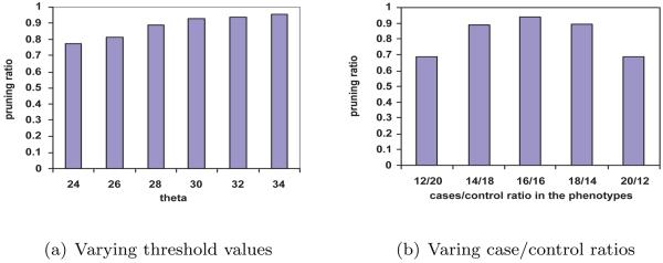
Figure 4(a) shows the fraction of SNP-pairs pruned under different thresholds. The pruning ratio is averaged over 20 random phenotype permutations. The datasets contain half cases (diseased individuals) and half controls (healthy individuals). A large portion of the SNP-pairs are pruned even when the threshold is low. Figure 4(b) show the pruning ratio of the SNP-pairs when the case/control ratio varies, while the total number of individuals is fixed. Clearly, the pruning effect reaches the maximum power when there are 16 cases and 16 controls, which demonstrates that FastChi is more suitable for balanced study.
Figure 4.
Pruning effect of the upper bound
Computational cost of each component of FastChi
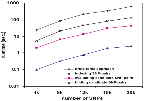
FastChi has three major components: building the indexing structure Array(Xi) for every SNP Xi, accessing Array(Xi) to find the candidate SNP-pairs whose upper bounds are greater or equal to the threshold, and performing chi-square tests on these candidates. Figure 5 shows the runtime of these three components when the number of SNPs increases. We also plot the runtime of the brute force approach for reference, which is the top line. Note that the runtimes in this figure are for a single permutation. As we can see, the most time consuming component of FastChi is building the index structures. Yet, its runtime is about 1/5 of the time required to perform the two-locus chi-square tests on all SNP pairs in one permutation. Note that when the number of permutations is large, the cost on building the index structures is negligible since they only need to be built once and can be reused in all permutations. Thus the performance gain of FastChi is more prominent for large permutation tests.
Figure 5.
Computational cost of each component of FastChi
5. Discussion
In this paper, we present the FastChi algorithm for genome-wide two-locus chi-square test. FastChi is an exhaustive method which guarantees to find the optimal solution. It utilizes an upper bound of the two-locus chi-square test value to prune a majority of the SNP-pairs. The upper bound developed in this paper can be easily incorporated in the algorithm for SNP-pair pruning and candidates retrieval. By eliminating redundant computation of the invariant units in each permutation, FastChi is even more effective than the brute force method in large permutation tests.
So far, we have described the method for given θ. The main goal of permutation test is to find threshold θ for a given family-wise error α′. FastChi can be easily modified for this task: For each permutation Yk, we use a parameter θk (initially 0) to track the largest chi-square value identified so far by the algorithm. The non-decreasing θk is then used as the threshold to prune the search space when the remaining SNP-pairs are examined.
FastChi can also benefit the two-stage genome-wide association study. The idea of the two-stage approache 4,19 is to first select a subset of important SNPs according to some criteria. Then in the second step, an exhaustive search is performed to find the interactions among the selected SNPs. FastChi can dramatically speed up the interaction analysis procedure in the second step. A much larger number of SNPs can now be selected in the first step for the subsequent interaction analysis.
In this paper, we mainly focus on the biallelic SNPs. For the heterozygous case (where SNPs are encoded using {0, 1, 2}), we can also derive a similar upper bound. Let A, B, E, C, D, F represent the following events respectively: Y = 0 ∧ Xi = 0; Y = 0 ∧ Xi = 1; Y = 0 ∧ Xi = 2; Y = 1 ∧ Xi = 0; Y = 1 ∧ Xi = 1; Y = 1 ∧ Xi = 2. The upper bound for χ2(XiXj, Y) is: χ2(XiXj, Y ) ≤ χ2(Xi, Y) + T1S1ℛ0 + T2S2ℛ1 + T3S3ℛ2. In the upper bound, , where a ∊ {0, 1, 2}, T1 = L/(OA + OC), T2 = L/(OB + OD), T3 = L/(OE + OF), (where L = M2/[(OA + OB + OE)(OC + OD + OF)]), .
In our future work, we will investigate association study involving more than two SNPs following the same principle discussed in this paper.
References
- 1.http://www.gnf.org/
- 2.Carlson CS, Eberle MA, Kruglyak L, Nickerson DA. Mapping complex disease loci in whole-genome association studies. Nature. 2004;429 doi: 10.1038/nature02623. [DOI] [PubMed] [Google Scholar]
- 3.Curtis D, North BV, Sham PC. Use of an artificial neural network to detect association between a disease and multiple marker genotypes. Ann. Hum. Genet. 2001;65:95–107. doi: 10.1046/j.1469-1809.2001.6510095.x. [DOI] [PubMed] [Google Scholar]
- 4.Evans DM, Marchini J, Morris AP, Cardon LR. Two-stage two-locus models in genome-wide association. PLoS Genet. 2006;2:e157. doi: 10.1371/journal.pgen.0020157. [DOI] [PMC free article] [PubMed] [Google Scholar]
- 5.Halperin E, Kimmel G, Shamir R. Tag snp selection in genotype data for maximizing snp prediction accuracy; Proceedings of the International Conference on Intelligent Systems for Molecular Biology; 2005. [DOI] [PubMed] [Google Scholar]
- 6.Herbert A, et al. A common genetic variant is associated with adult and childhood obesity. Science. 2006;312:279–284. doi: 10.1126/science.1124779. [DOI] [PubMed] [Google Scholar]
- 7.Nelson MR, Kardia SL, Ferrell RE, Sing CF. A combinatorial partitioning method to identify multilocus genotypic partitions that predict quantitative trait variation. Genome Research. 2001;11:458–470. doi: 10.1101/gr.172901. [DOI] [PMC free article] [PubMed] [Google Scholar]
- 8.Nicodemus KK, Liu W, Chase GA, Tsai Y-Y, Fallin MD. Comparison of type i error for multiple test corrections in large single-nucleotide polymorphism studies using principal components versus haplotype blocking algorithms. BMC Genet. 2005;6(Suppl 1):S78. doi: 10.1186/1471-2156-6-S1-S78. [DOI] [PMC free article] [PubMed] [Google Scholar]
- 9.Nyholt DR. Simple correction for multiple testing for single-nucleotide polymorphisms in linkage disequilibrium with each other. Am. J. Hum. Genet. 2003;74(4):765–769. doi: 10.1086/383251. [DOI] [PMC free article] [PubMed] [Google Scholar]
- 10.Ozaki K, et al. Functional snps in the lymphotoxin-alpha gene that are associated with susceptibility to myocardial infarction. Nat. Genet. 2002;32 doi: 10.1038/ng1047. [DOI] [PubMed] [Google Scholar]
- 11.Pagano M, Gauvreau K. Principles of Biostatistics. Duxbury Press; Pacific Grove, CA: 2000. [Google Scholar]
- 12.Province MA, Shannon WD, Rao DC. Classification methods for confronting heterogeneity. Adv. Genet. 2001;42:273–286. doi: 10.1016/s0065-2660(01)42028-1. [DOI] [PubMed] [Google Scholar]
- 13.Ritchie MD, Hahn LW, Roodi N, Bailey LR, Dupont WD, Parl FF, Moore JH. Multifactor-dimensionality reduction reveals high-order interactions among estrogen-metabolism genes in sporadic breast cancer. American Journal of Human Genetics. 2001;69:138–147. doi: 10.1086/321276. [DOI] [PMC free article] [PubMed] [Google Scholar]
- 14.Roberts A, McMillan L, Wang W, Parker J, Rusyn I, Threadgill D. Inferring missing genotypes in large snp panels using fast nearest-neighbor searches over sliding windows. ISMB. 2007 doi: 10.1093/bioinformatics/btm220. [DOI] [PubMed] [Google Scholar]
- 15.Roses A. The genome era begins. Nat. Genet. 2003;33(Supp2):217. [Google Scholar]
- 16.Sebastiani P, Lazarus R, Weiss ST, Kunkel LM, Kohane IS, Ramoni MF. Minimal haplotype tagging. PNAS. 2003;100(17) doi: 10.1073/pnas.1633613100. [DOI] [PMC free article] [PubMed] [Google Scholar]
- 17.Segr D, DeLuna A, Church GM, Kishony R. Modular epistasis in yeast metabolism. Nat. Genet. 2005;37:77–83. doi: 10.1038/ng1489. [DOI] [PubMed] [Google Scholar]
- 18.Sherriff A, Ott J. Applications of neural networks for gene finding. Adv. Genet. 2001;42:287–297. doi: 10.1016/s0065-2660(01)42029-3. [DOI] [PubMed] [Google Scholar]
- 19.Storey J, Akey J, Kruglyak L. Multiple locus linkage analysis of genomewide expression in yeast. PLoS Biology. 2005;8:e267. doi: 10.1371/journal.pbio.0030267. [DOI] [PMC free article] [PubMed] [Google Scholar]
- 20.Thomas DC. Statistical methods in genetic epidemiology. Oxford Univeristy Press; Oxford: 2004. [Google Scholar]
- 21.Wade CM, Daly MJ. Genetic variation in laboratory mice. Nat. Genet. 2005;37:1175–1180. doi: 10.1038/ng1666. [DOI] [PubMed] [Google Scholar]
- 22.Zhang H, Bonney G. Use of classification trees for association studies. Genet. Epidemiol. 2000;19:323–332. doi: 10.1002/1098-2272(200012)19:4<323::AID-GEPI4>3.0.CO;2-5. [DOI] [PubMed] [Google Scholar]
- 23.Zhang X, Zou F, Wang W. Fastanova: an efficient algorithm for genome-wide association study. KDD. 2008 [PMC free article] [PubMed] [Google Scholar]


