Intergenerational resource transfers with random offspring numbers

Abstract

A problem common to biology and economics is the transfer of resources from parents to children. We consider the issue under the assumption that the number of offspring is unknown and can be represented as a random variable. There are 3 basic assumptions. The first assumption is that a given body of resources can be divided into consumption (yielding satisfaction) and transfer to children. The second assumption is that the parents' welfare includes a concern for the welfare of their children; this is recursive in the sense that the children's welfares include concern for their children and so forth. However, the welfare of a child from a given consumption is counted somewhat differently (generally less) than that of the parent (the welfare of a child is “discounted”). The third assumption is that resources transferred may grow (or decline). In economic language, investment, including that in education or nutrition, is productive. Under suitable restrictions, precise formulas for the resulting allocation of resources are found, demonstrating that, depending on the shape of the utility curve, uncertainty regarding the number of offspring may or may not favor increased consumption. The results imply that wealth (stock of resources) will ultimately have a log-normal distribution.

There are many points of overlap between the fundamental theoretical questions in economics and those in evolutionary ecology, and these have been explored widely in both disciplines. Many problems in evolutionary theory, like the consumption of available resources, fit easily into this framework, and the insights from economics have illuminated core problems in behavioral ecology (see for example refs. 1–6). Similarly, ecological and evolutionary approaches can shed light on fundamental problems in economics (7–8).

Among the most classic challenges in both ecology and economics is how one discounts the future and trades off present consumption against discounted future rewards. In the economic context, this is a well-posed problem; the solution involves maximization, across a range of options, of the discounted present utility to be realized from that set of options. Analogous problems in evolutionary ecology involve the tradeoffs between growth and reproduction, and problems of parent-offspring conflict. For example, for annual plants, the earlier a plant switches from growth to reproduction, the longer it can spend reproducing; but the reduced resources at the onset of early reproduction translate into reduced production per unit time. In contrast, deferring the transition to reproduction too late can lead to insufficient time for producing offspring; the resolution of this tradeoff then involves, as is intuitively clear, transition at intermediate times from growth to reproduction (9). The coupling of timing of reproduction and parent-offspring conflict is explored more fully in ref. 10.

More generally, most of the central problems in evolutionary ecology involve resolution of life-history tradeoffs, such as those between growth and reproduction. Increased reproduction is generally at the expense of the survival of the parent. Early reproduction may increase the number of potential offspring one can have; furthermore, for a growing population with overlapping generations, offspring produced early in life are more valuable than those produced later because those offspring can also begin reproduction earlier. This is analogous to the classic investment problem in economics, in that population growth imposes a discount rate that affects when one should have offspring. The flip side is that early reproduction compromises the parent's ability to care for its children, and that increased number of offspring reduces the investment that can be made in each. Again, the best solution generally involves compromise and an intermediate optimum.

A particularly clear manifestation of this tradeoff involves the problem of clutch or litter size—how many offspring should an organism, say a bird, have in a particular litter? (11) Large litters mandate decreased investment in individuals, among other costs, but increase the number of lottery tickets in the evolutionary sweepstakes. This problem has relevance across the taxonomic spectrum, and especially from the production of seed by plants to the litter sizes of elephants and humans. Even for vertebrates, the evolutionary resolution shows great variation: The typical human litter is a single individual, for which parental care is high, whereas fish may produce millions of offspring with low individual probabilities of survival.

The great British biologist David Lack (12) provided a simple and intuitive solution to this problem: The optimal solution was predicted to maximize the product of the number of offspring and their probability of survival to reproduce. The problem with this solution is that it is incomplete: It ignores the carry-over effect from one generation to another, basically the grandparent effect. Although a large litter with low investment per offspring may lead to the same product as a small litter with high investment per offspring, the members of the smaller litter are also likely to be more fit, leading to a carry-over effect to future generations (see also refs. 3, 6, and 11). Livnat et al. (13) explore this question with a game-theoretic model, and show that the balance between large and small litters is affected fundamentally by the degree of genetic reassortment: When mutation (or recombination) rates are high, individuals are more weakly related to their offspring, and the best solution tends toward the production of large litters with small investment. When reassortment is low, as for humans, the balance shifts toward small litters and large investment per offspring.

Still, there is always some degree of reassortment, especially for diploid populations; hence, the problem of intergenerational transfers of resources becomes a fundamental issue in ecology and economics alike. All individuals are mortal, and so discounting of the future has to account for (i) whether an individual uses resources now or later and (ii) whether deferring consumption until the future increases the likelihood that those resources will be used by one's children, or others' children, versus by the individual who is deferring. These two related problems—the individual versus one's children, and one's children versus the children of others—are at the core of both estate planning and decisions about environmental protection. A related problem involving the coevolution of intergenerational transfers and life history is treated in ref. 14.

The dynasty model (see refs. 15 and 16 and, for a more general formulation, ref. 17), in which one's offspring are a continuation of self, is designed to account for these issues, and can also account for the distinctions between one's own utility and one's offspring's utilities. The remaining problem, however, is that dynasty models typically deal with deterministic futures in terms of the number of offspring per parent. Even if population growth is negligible, so that each parent on average is replaced by one offspring, in practice this does not mean that every individual is replaced by precisely one genetic partial copy. Some individuals will remain childless, whereas others will have large numbers of offspring. How does this uncertainty affect the decisions one makes regarding transfers? How does the variance of the probability distribution of offspring affect the optimal decision? What are the consequences, if individuals employ optimal strategies, for the distribution of wealth within a population? Will the differences among these distributions in different cultures reflect differences in reproductive patterns, and especially the variances in the reproductive kernels?

In this article, we introduce a framework to begin investigating this problem. We present here only a model of the simplest cases, leaving for future work (likely by others) problems such as the importance of information about future uncertainty in determining one's decisions about the intergenerational transformation of resources. For example, early in life, one has little information about the number of surviving offspring one will have; but that uncertainty diminishes with age. Of course, even grown offspring can die, leaving another source of uncertainty even late in life. Similarly, we know less about how many offspring our children will have, or our grandchildren will have, than we know about our own fecundity. A full theory will need to examine these, and other, effects.

Results

Basic Model.

The dynamic programming framework we use in this article, based on Bellman's equation, is standard in economics and behavioral ecology alike (see for example ref. 14), For simplicity, we ignore differences between the sexes, and assume a single-sex model. Each individual lives for 1 unit of time, and is endowed (by inheritance) with, say, K units of wealth, which can be divided between her own consumption and the estate. She gets satisfaction both from her own consumption and from the welfare of her heirs. Because we will assume the identical concave utility function for all offspring, the optimal strategy for maximizing total welfare divides the estate equally among the heirs, whose welfare is in general discounted compared with the individual's own consumption. Also, the estate grows by a constant factor, γ, over each period.

Let U(c) be the satisfaction (“utility”) that any individual receives from consumption, c. Now assume that the number of offspring n is a random variable, with the same distribution for all families and independently distributed across families. The total welfare, starting with initial capital, K, of any individual is her utility plus the welfare of each of her heirs, discounted by a factor, β (which is generally <1, but need not be). Hence, along the optimal path, consumption must be chosen such that the expectation V(K) of total welfare (expected sum of discounted utilities, including those of descendants) satisfies the Bellman condition (see refs. 18 and 19):

It is implicitly assumed that the individual knows how many heirs she has before choosing how to divide her wealth between her own consumption and her estate. Next, following the standard theory, we assume that U is a concave increasing power function, and for definiteness assume explicitly that

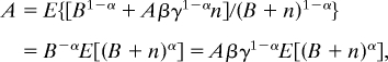
(U(c) is allowed to be negative if α > 1, because only relative utility matters). To solve the dynamic programming problem given by Eq. 1 and 2, conjecture the ansatz that

for some A. Substitution will confirm that the ansatz satisfies the problem, and determine A. Then the optimization yields,

and therefore,

where

Then the capital, K′, of each of the heirs is given by

We still have to verify that our ansatz (Eq. 3) holds for some A. Substitute for c from Eq. 4 into Eq. 1, using Eqs. 2, 3, and 5. The factor, K^{1 − α}/(1 − α), appears on both sides and can be cancelled out. Then, we have

so that B is determined by the equation

the appropriate A then is determined from Eq. 5, so that the conjecture is verified.

Note that the condition that there exists an optimal solution is the same as that Eq. 7 has a solution. Because the left-hand side is a strictly increasing function of B and approaches infinity with B, the existence condition is that

This condition can be interpreted as stating that β cannot be too large: If too much weight is placed upon the welfare of future generations, we would be led to the paradoxical situation that none of the resource should be consumed, leaving all for future generations whose optimal strategy, however, similarly is to use none. Note further that the limiting case where α = 1 reduces, by L'Hospital's rule, to U(c) = ln(c). In that case, Eq. 7 reduces to the simple equation

Finally, note that Eq. 7 can be used to compare the stochastic and deterministic cases, because in the deterministic case the expectation is simply the value of (B + n)^α. Therefore, from Eq. 7 we get that, E((B + n)^α) = (B₀ + E(n))^α, where B₀ is the solution to the problem when the mean number of children is the same but there is no variation.

If α < 1, the function (B + n)^α is concave in n, so that, by Jensen's inequality,

and therefore,

Similarly,

That is, if utility of additional consumption falls off relatively slowly (α < 1), then uncertainty about the number of one's heirs selects for higher consumption; but, if utility of additional consumption falls off rapidly, uncertainty selects for lower consumption.

Implications for the Distribution of Wealth.

Computation of the optimal policy does not deviate a great deal from the deterministic theory, but there are interesting implications for the pattern of distribution of wealth. The essential relation is Eq. 6. Start with a set of individuals at generation t, each with a capital stock (so we have a distribution of capital ownership). For each such individual, draw n at random (independently across individuals across time). Those individuals for which n > 0 generate n new entities, each with a capital given by Eq. 6. Thus, the distribution at generation t is transformed into a new distribution at generation t + 1. Can we say anything interesting about this, for example, about the limiting distribution?

In our model, for any individual with capital stock, K, and n offspring, each offspring has capital stock, K′ = γ K/(B + n), where γ is the increased capital per unit of initial capital, and B is a parameter. The random variable, n, has a given distribution, independent of K.

If p(n) is the probability of n offspring, then, among parents with capital K, the observed distribution of K′(n) will be given by q(n) = np(n)/E(n).

Let k′ = ln K′, k = ln K, and u(n) = ln γ − ln(B + n). The distribution of u(n) in the next period then is given by q(n). Hence,

Here, k and u are independent variables. In the case when p(n) is positive for exactly 1 positive n, all surviving families will have the same number of offspring, and hence there will be no spread of wealth. More generally, however, Eq. 9 implies a random-walk process for which

By the central limit theorem,

converges to a limit random variable with mean 0 and variance 1; and furthermore, k, properly normalized as above, converges to a normal distribution, or K to a log-normal distribution. This is illustrated by simulations (Fig. 1), for representative values of the parameters chosen so that the expected change in the mean of log wealth is zero. An analogous case, where n is fixed at 1 but γ is a random variable, was first studied by the French engineer Robert Gibrat (20); the result is usually referred to as Gibrat's Law.

Fig. 1.

Normalized distribution of log wealth after 100 generations, compared with the normal distribution, for B = 1 and probabilities 7/18, 6/18, 3/18, and 2/18, respectively, of 0, 1, 2, and 3 offspring.

Overlapping Generation Growth with Random Family Size.

Until this point, we have assumed that individuals make decisions about the distribution of wealth once in their lifetime and with full knowledge of how many offspring they will have among whom to divide resources. More generally, however, the allocation problem is a continuous one, and the solutions temporally variable as information accrues about the number of offspring, and as expected conditional life expectancy diminishes. To examine this problem, we approximate the continuous decision process with a 2-stage model in which the parent's resources can grow for one period and then be used for consumption and production of children.

We retain some of the basic elements of the previous models. The utility of consumption, c, in any period is a power function, c^{1 − α}/(1 − α). Capital in any one period is divided between consumption and savings; savings after one period are multiplied by a growth factor, γ. Each individual lives and consumes for 2 periods, and discounts second-period welfare by a factor, δ. “Welfare” here includes both the utility of second-period consumption of the parent and the long-term welfare of the children. In the second period of a parent, the random number of children, n, is known. The parent divides the capital available to her between consumption for self and capital to the children. Each child receives an equal endowment. Each child then immediately chooses first-period consumption as the parent had done. The parent discounts each child's welfare compared with her own (this applies instantaneously) with a factor, β (again, we do not of course exclude that there is no real discounting, i.e., one or the other of the discount rates might equal or even exceed 1).

Let V(K) be the welfare (i.e., expected sum of discounted utilities, including those of descendants) for an individual with capital K. Let c₁ be the consumption of the parent in period 1 and K′ be capital of the parent at the beginning of period 2, i.e.,

Let c₂ be the consumption of the parent in period 2. Then, if there are n children, the initial capital of each child is

Hence,

Now, let us make explicit the assumptions about knowledge of n. Assume that at period 2, the parent knows the actual realization of n; but that in period 1, the parent does not (although the parent does know the distribution of n). In period 2, then, we optimize on c₂, given K′, which has been determined by the choice of c₁, and given n. This choice determines a second-period payoff (the expression in curly brackets) as a function of n and c₁. Take the expectation of this payoff with respect to n; we then have 2 functions of c₁, whose weighted sum is to be maximized.

To simplify the later discussion, it is convenient to state a general lemma about functions of this kind, which we will use twice in the following analysis.

Lemma.

Let φ(c) = [c^1−α/(1 − α)] + P[(K − c)^1−α/(1 − α)], where P is a positive constant. Then φ(c) is maximized at c = [Q/(1 + Q)]K, where Q is defined by Q^−α = P, and the maximum value of φ is P(1 + Q)^αK^1−α/(1 − α).

The result follows straightforwardly from setting the derivative φ′ equal to zero (note that φ is a concave function) and then substituting.

We now proceed as before. Conjecture that

for some A, then show that we can find a value of A such that Eq. 14 is satisfied.

Consider first the second-stage optimization, where n is known and c₂ is chosen.

Note that V(K″) = An^{α − 1} (K′ − c₂)^{1 − α}/(1 − α), so that, from Eq. 14, c₂ maximizes,

where P₂ = Aβn^α. Define B by

Then, if we define Q₂ in terms of P₂ as in the Lemma, we see that,

Then,

and

From the second part of the Lemma, we find that,

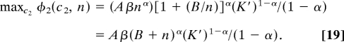Now we proceed to the determination of c₁. Because n is unknown at time 1, we substitute the expected value of Eq. 19 for the expression in curly brackets in Eq. 14.

Let

Substitute from Eq. 19 and then substitute for K′ from Eq. 12.

where

Define C by

For any positive random variable, X, we can define the α-mean of X by

Then, if we define Q₁ in terms of P₁ as in the Lemma, we see that,

Hence, by the Lemma,

and

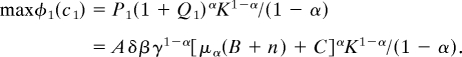Because this has to equal V(K) by the Bellman equation, we conclude that

We can express C in terms of B and so reduce Eq. 21 to an equation in one unknown. Divide Eq. 20 by Eq. 15 and then raise both sides to the power, −1/α:

Then Eq. 21 becomes, after some simplification,

The left-hand side is a strictly increasing function of B and approaches infinity as B approaches infinity. Hence, Eq. 23 has a unique solution if the left-hand side is <1 at B = 0, i.e., if

From Eqs. 21 and 22 and the formula for c₁, we can write

We can then derive the law of motion of the capital stock of each individual by substituting into Eq. 12 and then Eq. 18.

This is the initial capital of each child when the parent's capital is K. Once again, it leads to the conclusion that the asymptotic distribution of wealth is log-normal.

Discussion

It is not surprising that fundamental problems in economics have strong analogies to similar problems in evolutionary ecology. In both realms, individuals must trade off current and future discounted benefits, to themselves and to others. Evolution favors those strategies that increase payoffs, and the solutions evolution favors broadly should be represented in the ways individuals make decisions, for example about current consumption versus savings for the future and legacies for offspring. Fundamental in both arenas is how uncertainty affects decisions, and when it selects for higher discounting of future benefits. We explore this issue through a generalization of standard consumption models to uncertain environments, providing a framework that we hope will serve as a springboard for further studies.

The general problem addressed in this article is how an individual should allocate resources to maximize her expected total welfare, where the decision must balance current consumption and future consumption by one's offspring, whose own welfare is discounted relative to the parent's. What is unique about our model is that the number of offspring one has is not fixed but is a random variable drawn from a distribution. We begin with the simplest case, in which individuals have full knowledge of how many offspring they will have before making the consumption decision, and then extend that result to the case when decisions are made twice in one's lifetime, the first with no knowledge. Because of the specific form assumed for the utility function, we are able to derive an explicit analytical solution to the problem (using Bellman's equation). Depending on the specific form of the utility function, the uncertainty introduced by the randomness in number of offspring may either increase or decrease current consumption. Finally, implementing the optimal solution leads to a log-normal distribution of wealth, with a variance that increases with time proportionally to the weighted variance in the offspring distribution.

References

- 1.Maynard Smith J. Evolution and the Theory of Games. Cambridge, UK: Cambridge Univ Press; 1982. [Google Scholar]
- 2.Schoener T. The theory of feeding strategies. Annu Rev Ecol Syst. 1971;2:369–404. [Google Scholar]
- 3.Mangel M, Clark CW. Dynamic Modeling in Behavioral Ecology. Princeton: Princeton Univ Press; 1988. [Google Scholar]
- 4.Charnov EL. Optimal foraging: The marginal value theorem. Theor Pop Biol. 1976;9:129–136. doi: 10.1016/0040-5809(76)90040-x. [DOI] [PubMed] [Google Scholar]
- 5.Stephens DW, Krebs JR. Foraging Theory. Princeton: Princeton Univ Press; 1987. [Google Scholar]
- 6.Houston A, Clark CW, McNamara JM, Mangel M. Dynamic models in behavioural and evolutionary ecology. Nature. 1988;332:29–34. [Google Scholar]
- 7.Dasgupta P, Maskin E. Uncertainty and hyperbolic discounting. Amer Econ Rev. 2005;95:1290–1299. [Google Scholar]
- 8.Becker G. Altruism, egoism and genetic fitness: Economics and sociobiology. J Eco Lit. 1976;14:817–826. [Google Scholar]
- 9.Cohen D. The optimal timing of reproduction. Am Nat. 1976;110:801–807. [Google Scholar]
- 10.Einum S, Fleming IA. Selection against late emergence and small offspring in Atlantic salmon (Salmo salar) Evolution. 2000;54:628–639. doi: 10.1111/j.0014-3820.2000.tb00064.x. [DOI] [PubMed] [Google Scholar]
- 11.Clark CW, Mangel M. Dynamic State Variable Models in Ecology: Methods and Applications. New York: Oxford Univ Press; 2000. [Google Scholar]
- 12.Lack D. The significance of clutch size. Ibis. 1947;89:302–352. [Google Scholar]
- 13.Livnat A, Pacala SW, Levin SA. The evolution of intergenerational discounting in offspring quality. Am Nat. 2005;165:311–321. doi: 10.1086/428294. [DOI] [PubMed] [Google Scholar]
- 14.Chu CYC, Lee R. The co-evolution of intergenerational transfers and longevity: An optimal life history approach. Theor Pop Bio. 2006;69:193–201. doi: 10.1016/j.tpb.2005.11.004. [DOI] [PMC free article] [PubMed] [Google Scholar]
- 15.Meade JE. Trade and Welfare. London: Oxford Univ Press; 1955. Chapter VI. [Google Scholar]
- 16.Arrow KJ, Kurz M. Public Investment, the Rate of Return, and Optimal Fiscal Policy. Baltimore: Johns Hopkins Univ Press; 1980. Chapter I, section 4. [Google Scholar]
- 17.Becker GS, Barro RJ. A reformulation of the economic theory of fertility. Q J Econ. 1988;103:1–25. [PubMed] [Google Scholar]
- 18.Bellman R. Dynamic Programming. Princeton: Princeton Univ Press; 1957. p. 11.p. 64.p. 70. [Google Scholar]
- 19.Duffie JD. Dynamic Asset Pricing Theory. Princeton: Princeton Univ Press; 2001. p. 62.p. 66. [Google Scholar]
- 20.Gibrat R. Les inégalités économiques. Paris: Sirey; 1931. [Google Scholar]