Measurement error caused by spatial misalignment in environmental epidemiology

Abstract

In many environmental epidemiology studies, the locations and/or times of exposure measurements and health assessments do not match. In such settings, health effects analyses often use the predictions from an exposure model as a covariate in a regression model. Such exposure predictions contain some measurement error as the predicted values do not equal the true exposures. We provide a framework for spatial measurement error modeling, showing that smoothing induces a Berkson-type measurement error with nondiagonal error structure. From this viewpoint, we review the existing approaches to estimation in a linear regression health model, including direct use of the spatial predictions and exposure simulation, and explore some modified approaches, including Bayesian models and out-of-sample regression calibration, motivated by measurement error principles. We then extend this work to the generalized linear model framework for health outcomes. Based on analytical considerations and simulation results, we compare the performance of all these approaches under several spatial models for exposure. Our comparisons underscore several important points. First, exposure simulation can perform very poorly under certain realistic scenarios. Second, the relative performance of the different methods depends on the nature of the underlying exposure surface. Third, traditional measurement error concepts can help to explain the relative practical performance of the different methods. We apply the methods to data on the association between levels of particulate matter and birth weight in the greater Boston area.

1. INTRODUCTION AND SCIENTIFIC MOTIVATION

Exposure assessment studies have shown that there exist important factors, such as traffic conditions, point sources of pollution, and urban building canyon effects, that induce spatial variability in pollution levels. With the advent of geographic information system (GIS)-based modeling, researchers have begun to focus on spatial variability in air pollution and its relationship with human health (Berhane and others, 2004, Zidek and others, 2004, Kunzli and others, 2005, Gryparis and others, 2007). Such spatial analyses have several advantages over studies that assign exposure readings from a central-site monitor to all study participants. First, spatial analyses do not assume that exposure is constant over the region of interest, thereby reducing exposure measurement error that would otherwise lead to a loss of power. Second, in the case of chronic diseases, analyses rely primarily on exposure heterogeneity induced by spatial variability. Finally, it is now widely recognized that air particulates are a complex mixture of multiple sources of pollution, with pollution from each source having a distinct chemical profile and perhaps different toxicity. Because pollutants from different sources have different spatial distributions, with regional pollutants (e.g. sulfates from coal-fired power plants) being more homogeneous over space and local sources (e.g. black carbon[BC] from traffic emissions) demonstrating higher spatial variability, incorporation of the spatial variability of local pollutants in a health effects analysis may help separate health effects from different sources.

In many such studies, the locations of the exposure data and those of the health data do not coincide. Standard regression methods cannot be applied to such misaligned data. To overcome this problem, several methods have been proposed. Most approaches involve directly using predictions from statistical exposure models that incorporate spatial structure (Shaddick and Wakefield, 2002, Kunzli and others, 2005, Gryparis and others, 2007). Higgins and others (1997) used polynomial regression to generate covariate predictions when outcomes and covariates were misaligned in time. Waller and Gotway (2004) used kriging to predict exposures and used resampling to account for the uncertainty in using the predictions in place of the true values. They classified predicted exposures as high, medium, or low and fitted multiple health regressions using the simulated categorical exposures as covariates. Kunzli and others (2005) assigned exposure values for subject-specific locations derived from a geostatistical model and used weighted least squares in the subsequent health effects model, with the weights specified as the inverse of the standard errors (SEs) from the exposure kriging model. For this same problem, Madsen and others (2008) considered both a generalized least squares (GLS) estimator with a bootstrap-type variance estimator and a maximum likelihood approach that jointly fits the exposure and health models.

In this paper, we evaluate and compare approaches to fitting linear and logistic health models with predicted exposures, including approaches specifically suggested for this setting as well as several modified approaches motivated by measurement error principles. We first use a very simple linear model to illustrate measurement error issues associated with spatially misaligned exposure and health point data. This simple structure is instructive in demonstrating the relative strengths and weaknesses of the various methods proposed for dealing with this type of data, which commonly arises in chronic and within–urban area studies of the health effects of air pollution. We then consider nonlinear models under the generalized linear model framework, focusing on logistic regression.

The structure of this paper is as follows. In Section 2, we introduce our notation. In Section 3, we discuss how smoothing converts classical measurement error to Berkson error and the implications of this. In Sections 4 and 5, we describe and analytically evaluate the multiple approaches to the problem for continuous and binary outcomes, respectively. In Section 6, we present a simulation study to further compare the methods. In Section 7, we describe an application of the methods to data on the association between traffic particle levels and birth weights in the greater Boston area. We conclude with discussion in Section 8.

2. MODELING FRAMEWORK

To introduce our notation, let X be the vector of the true exposures and W be the vector of its error-prone, but not misaligned, measurements. Moreover, let S be the vector of smoothed estimates of X based on W, U = W − X the vector of measurement errors, V = X − S the vector of the error after the smoothing procedure, and Y the health response. Let (·)^* indicate the values at locations without exposure observations; for example, Y^* is the vector of health observations at locations without exposure data.

In what follows, we assume that Y_i^* given X_i^* and Z_i^* are independent random variables having a distribution in the natural exponential family (McCullagh and Nelder, 1989). Let μ_i^* = E(Y_i^*|X_i^*,Z_i^*). We assume the following model holds:

(2.1)

(2.2)

where g(x) is a monotonically increasing link function, β₁ and β_z are unknown parameters, and the measurement errors U_i are independent of Y_i^* given X_i^* and Z_i^*. In the above equation, X_i^* is the exposure (e.g. air pollutant level) at the residence of the ith subject, over some biologically relevant period of interest, and Z_i^* is a q×1 vector of covariates measured without error. In this work, we treat X as correlated in space although in spatiotemporal settings X could also be serially correlated over time. W_i represents an exposure measurement, which may or may not differ from X_i, depending on whether or not instrument error is present. In the misalignment scenario, the variable X = (X₁,X₂,…,X_nw)^T is measured with error by W = (W₁,W₂,…,W_nw)^T at different points in space than the variable Y^* = (Y₁^*,Y₂^*,…,Y^*n_y)^T. Hence, to estimate exposure, we obtain smoothed predictions S^* = (S₁^*,S₂^*,…,S^*n_y)^T of the unobserved X^* = (X₁^*,X₂^*,…,X^*n_y)^T from an exposure model. Scientific interest then focuses on β₁, the regression coefficient relating exposure and health.

An important aspect is the nature of the error in the stochastic exposure process. We decompose the process as

where g(·) represents a smooth spatial surface and δ(·) is an additive uncorrelated error with variance σ_δ² that accounts for fine-scale heterogeneity in the exposure. In this case, the measurement error U represents instrument error. Unless multiple measurements at a given site and time are available, one cannot resolve the fine-scale heterogeneity δ in the presence of U as the model cannot inform both σ_u² and σ_δ² (Cressie, 1993, p. 59). In air pollution studies, we believe that most of the unexplained variability is fine-scale heterogeneity and not instrument error, such that σ_u²≈0 and Var(δ_i + U_i)≈σ_δ².

3. SMOOTHING-INDUCED BERKSON ERROR

In this section, we argue that the plug-in approach that uses smoothed predicted values of exposure as covariates in a health effects model is a form of regression calibration that produces a Berkson structure (Carroll and others, 1995) in the health model. Exposure estimates most often are generated using one of the many approaches to spatial smoothing, such as kriging and its extensions (Cressie, 1993), Gaussian process (GP) modeling and Bayesian smoothing (Gaudard and others, 1999; Banerjee and others, 2004), penalized regression splines (Kammann and Wand, 2003; Ruppert and others, 2003; Gryparis and others, 2007), and kernel smoothing (Hobert and others, 1997), among others. For concreteness, consider a Bayesian framework in which we place a GP prior on X(·): X(·)~GP[μ(·),R(·)]. Hence,

The interim posterior (before any health analysis) for the conditional distribution of X^* given W is

(3.1)

In a measurement error framework, the interim posterior mean takes the form of a regression calibrator, representing the mean of the unobserved covariate given the observations W. As all regression calibrators do, use of this estimator turns around the conditioning and yields a Berkson framework whereby the distribution of an unknown value X_i^* is centered around the posterior mean, as shown in (3.1). The term multiplying W in (3.1) is the spatial analog of , which is the familiar correction factor in the simplest independent measurement error setting, but the covariance accounts for the spatial covariance structure. Assuming the covariance structure is known, then as in a standard Berkson model, the ordinary least squares (OLS) estimator based on a regression model using E(X_i^*|W) as a covariate is unbiased. We can write

(3.2)

where V^* = (V₁^*,V₂^*,…,V_ny^*)^T has mean zero and variance–covariance matrix Σ^* equal to the posterior variance given above. For a given degree of smoothing, other smoothers should give a similar decomposition. That is, if the data are really generated from a GP with known variance components and we use the best linear unbiased predictors (BLUPs) for our exposure predictions, then the Berkson error analogy holds exactly. However, in reality, the data do not come from a GP with known variance components, and so this analogy does not hold exactly. Other smoothing techniques will create a structure analogous to Berkson error in that the smoothed predictions will have a smaller variance than the observed data and the covariance of V_i^* and E(X_i^*|W) will be small. Thus, the analytic results obtained in the simple GP setting for which exact results exist lend insights into the likely performance of predictions obtained by other smoothers generally. For instance, the kriging estimator is the BLUP of X^* and is equivalent to (3.1). Similarly, estimated smooths from regression splines, including spatial smoothing, are also BLUPs within a mixed model framework (Ruppert and others, 2003). Thus, each approach will approximately produce a decomposition X^* = S^* + V^*, in which V^* is orthogonal to S^*, as in (3.2). For an empirical example of such structure, see Paciorek and others (2008). In the case of spatial smoothing, with X^* = S^* + V^*, note that the residual term, V^*, does not have a diagonal covariance structure. The uncertainty in X^*, as captured by the covariance matrix Σ^* = Var(X^*|W), is spatially correlated and heteroscedastic. Note that Σ^* should include any component σ_δ² but not σ_u².

For the general health model (1), even when the variance components of the spatial exposure process g(·) are known, standard approaches to estimation do not yield unbiased estimates of β₁ (Carroll and others, 1995). However, closed-form expressions for this bias under the most general form of this model are unavailable, except for certain special cases. We now focus on 2 such special cases in the following 2 sections.

4. LINEAR HEALTH EFFECT MODEL

We now consider the special case of (2.1) when Y_i^* is normally distributed. Interest focuses on the linear regression model

(4.1)

We assume the errors, ϵ_i, are independent of the measurement errors, U_i. The remainder of this section describes 2 existing approaches, a plug-in estimator and an exposure simulation, as well as 2 approaches, regression calibration and Bayesian methods, drawn from the measurement error literature but not yet applied in the spatial setting. Section 6 compares these approaches in a simulation study. We also considered 2 other approaches, standard weighted least squares and an iterative GLS method, but relegate discussion of these to Section A of the supplementary material to this article, available at Biostatistics online at http://www.biostatistics.oxfordjournals.org.

4.1. Plug-in approach

The plug-in approach fits the exposure model for [X^*|W] and uses the predictions S^* as a covariate in the health model, which is fitted using OLS. By using S^* instead of X^* in the health model, we induce correlation: Y^* = β₀ + β₁X^* + ϵ = β₀ + β₁(S^* + V^*) + ϵ = β₀ + β₁S^* + η, where η = β₁V^* + ϵ. The new error term η no longer has a diagonal covariance matrix. Thus, although the OLS estimator for β₁ is unbiased, the variance estimator is incorrect since it does not account for the correlated, heteroscedastic error structure (Carroll and others, 1995, p. 63). To address this, one could use GLS to account for the induced covariance in the health model. Although it seems intuitive to use the uncertainty estimates from the exposure model (i.e. the elements of the diagonal in Σ^*) as the weights for the health model via simple weighted least squares, these are not the correct weights under the induced Berkson model. Since η = β₁V^* + ϵ and ϵ~N(0,σ_ϵ²In_y), it follows that the residual variance for the health model is given by β₁²Σ^* + σ_ϵ²In_y.

In practice, the variance components or smoothing parameters are not known, and we must estimate the parameters that govern the degree of smoothing. If we over smooth, the OLS estimator from the health model may be biased (Wakefield and Shaddick, 2006), with more bias occurring in situations in which it is difficult to estimate the appropriate amount of smoothing in the exposure model. Such scenarios include sparse monitoring data in a subregion or exposures that are very heterogeneous in space. Bias can also occur if the residual, V^*, is correlated with confounders, Z^*, in the health model, such as might result from correlation of confounders and exposure at small spatial scales.

4.2. Exposure simulation approach

Some have proposed an exposure simulation approach as an attempt to correct the variance of the plug-in estimator. Under this approach, M samples X_(t)^* = S^* + V_(t)^*, t = 1,2,…,M, are generated from the estimated distribution of exposure, given the data, and each of these M samples is used as a predictor to fit the health model. This yields M health effect estimates, , t = 1,2,…,M, which are then averaged to obtain an overall estimate. The corresponding variance of is equal to Var() = Var(E()) + E(Var()). Although Waller and Gotway (2004) used quantiles of simulated exposures, we consider direct use of the simulated exposures in the health model.

A simple analysis based on the Berkson framework we presented in Section 3 (supported by the results of our simulations in Section 6) indicates that rather than adjusting for the uncertainty induced by using the predicted exposures, such an approach induces bias in a linear health model. To illustrate, consider the samples X^*_(t) = S^* + V_(t)^*, t = 1,2,…,M. We have argued that the use of S^* should result in nearly unbiased health effect estimators. By adding V_(t)^*, one adds error to a variable that, if used on its own, yields unbiased estimates in the health model. Hence, this approach converts the problem back to the classical measurement error setting, where instead of using a covariate that yields unbiased results, measurement error in the covariate produces biased estimates. The size of the bias depends on the size of Σ^*. Therefore, we recommend against this approach. One can also view this problem from a multiple imputation perspective, where an appropriate exposure simulation scheme should take into account all available data and hence resample from the posterior predictive distribution of [X^*|W,Y^*] (Rubin, 1987). By using the conditional distribution [X^*|W], we discard the information for X^* in Y^*, resulting in an incorrect imputation scheme.

4.3. Out-of-sample regression calibration estimator

In many cases, it may be that spatial smoothing results in S^* being a biased estimate of the unknown expectation E(X^*|W). Departure from the simple X = S + V measurement error model may occur for several reasons, including poor estimation of the smoothing parameters and sparse exposure data in regions with health data.

Let (·)^** indicate the values at locations where exposure is observed but held out of the main model fitting for assessing model prediction. Hence, X^** is the vector of exposure measures that are held out from the exposure model, S^** the smoothed estimates that correspond to these locations based on the remaining exposure data, and Z^** is the matrix of covariates measured without error that correspond to these locations. We use the held-out data to fit a calibration of X^** to S^** and Z^**. We assume a simple measurement error model, in the spirit of Carroll and others (1995), of the form:

(4.2)

where E(ϵ_x,i) = 0 and Var(ϵ_x,i) = σ_x². By fitting model (4.2), we obtain the parameter estimates 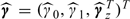, which we use to calibrate the predicted exposures S^* at the locations of interest. Hence, this method is an out-of-sample regression calibration (RC-OOS) approach, which has been described by Thurston and others (2003) in the context of a study design that corrects for measurement error by incorporating external validation data. In our case, we use it to correct for possible bias in our predictions. Define the matrices

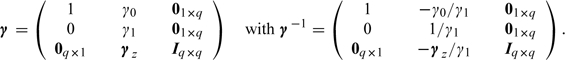Then, using (4.2), we have that E(X_i^*) = γ₀ + γ₁S_i^* + γ_z^TZ_i^*. We replace (γ₀,γ₁,γ_z) by and then calculate new estimated exposures, 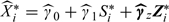, which we plug into the health model. This is equivalent to estimating 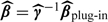, where β = (β₀β₁β_z^T)^T and _plug-in is the estimate from the plug-in model. It can be shown (Thurston and others, 2003) that the corrected β estimate is equal to

(4.3)

where D^* = [1|S^*|Z^*] and 1 is a vector of 1s. The variance of can be derived using either the sandwich method or a Taylor series expansion (Thurston and others, 2003). Both methods result in

(4.4)

In practice, especially if the number of exposure locations is not large enough to support holding out a sizable subset of locations, one could consider cross-validation to estimate the predicted exposures S_i^**, although simulation studies we conducted (results not shown) indicate that this approach does not perform as well as out-of-sample validation.

4.4. Bayesian approaches

In the fully Bayesian approach, one fits a joint model for the health and the exposure data. A fully Bayesian measurement error model adjusts in a natural way for the extra uncertainty associated with using the predicted exposure values in the health model and provides us with a correct variance estimate (Berry and others, 2002). Also, heteroscedasticity and correlation among exposure values are naturally incorporated in a Bayesian model through the uncertainty in X^*. The fully Bayesian model samples from the distribution [X^*,β|Y^*,W,Z^*]. Thus, in this model, when we update the unobserved exposure X^*, we use information from the health data Y^* along with that from the proxy W, which results in a proper multiple imputation scheme (Little, 1992).

In practice, we expect the number of exposure monitoring locations to be relatively small compared to the locations from which we have health data. In such cases, the health data could be very influential in determining the exposure predictions (Shaddick and Wakefield, 2002; Wakefield and Shaddick, 2006). If there are outliers in the health outcomes, especially if they correspond to locations for which we do not have adequate exposure information, then they could strongly affect the exposure surface. Other forms of model misspecification in either the exposure or the health model could also result in the exposure surface being overly influenced by the health observations, a situation similar to that in Yucel and Zaslavsky (2005) and for which the approach of “cutting feedback” has been suggested (Rougier, 2008). Poor estimation of the exposure surface could in turn affect estimates of the health effects.

An alternative to the fully Bayesian approach is a 2-stage Bayesian approach. In this approach, the first-stage model is the exposure model [X^*|W]∝[W|X^*][X^*] and the second-stage model is the health model [X^*,β|W,Y^*,Z^*]∝[Y^*|X^*,W,Z^*,β][X^*|W][β], where we use the interim posterior from the exposure model [X^*|W] as a prior distribution for X^* in the health model. The main difference between the 2 Bayesian approaches is that in the 2-stage Bayesian approach, we use a normal distribution for the interim posterior of X^* and numerically estimate its covariance matrix, whereas the fully Bayesian approach uses the exact version of this distribution by virtue of fitting the models jointly. The difference between this approach and the plug-in model is that the prior for X^* in the health model, which is the posterior for X^* from the exposure model, accounts for the uncertainty in X^*, including correlation and heteroscedasticity. We note that this 2-stage approach does not cut feedback between the health observations and the exposure estimates since the prior distribution for the exposure values is updated in the second stage. When the exposure model is complicated or when one is interested in running multiple epidemiological models, with different sets of covariates either for a single outcome or multiple outcomes, this 2-stage approach has the advantage that one does not have to refit the exposure model when running multiple health effect analyses.

5. GENERALIZED LINEAR MODELS FOR BINARY HEALTH OUTCOMES

Interest may also focus on the use of exposure predictions from spatially misaligned exposure data in generalized linear models for discrete outcomes (e.g. a binary or a count variable). Again, consider the Berkson error structure X_i^* = E(X_i^*|W) + V_i^*. Unlike the linear regression case, even under the correct amount of smoothing (e.g. if the variance components of the spatial exposure process are known), model fitting under this Berkson error structure does not yield unbiased estimates of β₁ (Carroll and others, 1995). Although it is difficult to obtain analytical expressions for the bias, closed-form expressions are available for certain special cases.

First, for simplicity, suppose the V_i^* are uncorrelated and homoscedastic. For a probit model for binary responses, the model based on the mean of the estimated exposure given the observed data is

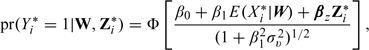(5.1)

where σ_v² is the variance of V_i^*. Therefore, the plug-in estimator obtained by fitting pr(Y_i^* = 1|W,Z_i^*) = Φ[β₀ + β₁E(X_i^*|W) + β_zZ_i^*] can yield bias, although the denominator on the right-hand side of (5.1) suggests that this bias will be small unless both σ_v² and β₁ are relatively large. Bias expressions in the analogous logistic model are typically approximated using the approximate relationship between the logistic and probit links (Carroll and others, 1995, (7.16)). When the V_i^* are heteroscedastic and correlated (as is the case for spatially misaligned data), even in the probit case, the marginal distribution of [Y^*|W,Z^*] involves an intractable multivariate probit integral. See Ochi and Prentice (1984) for a discussion of this issue for an equicorrelated multivariate probit model and Chib and Greenberg (1998) and De Iorio and Verzilli (2007) for Bayesian approaches to this problem.

6. SIMULATIONS

To compare the different methods, we performed a simulation study. For each scenario, we used N = 500 simulated data sets. For each data set, we used the geocodes of the n_w = 82 monitoring stations used in a recent Boston study (Gryparis and others, 2007) as the fixed exposure locations. We generated our exposure measurements, W, with no instrument error U, using W = X = g + δ, with g~N(μ1,R(ρ,ν)), where for R we used the Matérn correlation function. Specific parameter values depended on the exposure scenario, which we describe shortly. For the local heterogeneity δ, we assumed a mean-zero normal distribution with i.i.d. errors, σ_δ²In_w. We considered both continuous and binary outcomes, discussed separately in Sections 6.1 and 6.2.

6.1. Continuous outcomes

As noted in Section 4.4, the number of subjects on which health outcomes are measured is typically larger than the number of the exposure locations. Hence, for the linear model, we set n_y = 200. For the distribution of the health data, Y^*, we assume Y^*~N(β₀ + β₁X^*,σ_ϵ²In_y). We set β₀ = 0 and β₁ = 1 for all scenarios except the last, in which we set β₀ = β₁ = 0 in order to check the type-I error of each approach. We also ran simulations assuming incrementally smaller values of β₁, but the relative performances of the various approaches remained the same as that reported below and the relative bias changed little with different effect sizes (not shown). The assumption of independent health errors implies that the only component responsible for spatial autocorrelation of the health outcome is the exposure.

We considered 4 exposure scenarios. Scenario A corresponds to a very smooth surface, Scenario B a moderately smooth surface, while Scenario C (the roughest surface) is much more heterogeneous and therefore quite challenging to estimate. Figure 1 shows one realization of the true exposure surface, X, obtained from each of the above scenarios. Scenario D is the same as Scenario C, except exposure is not causally related to health (β₁ = 0). More details on the simulations are given in Section B of the supplementary material available at Biostatistics online.

Fig. 1.

Realizations of the true smooth exposure surface g(·) for simulation scenarios A, B, and C, on the [0,1]×[0,1] grid.

We used the methods described in Section 4 to fit the data sets generated under the above scenarios. First, we applied the plug-in approach, estimating the smooth exposure surface using the spm function in the SemiPar package (Wand, 2008) in R. This function uses a mixed model representation of penalized regression splines, described in more detail in Section C of the supplementary material available at Biostatistics online. The degrees of freedom for the spatial component was chosen by the default method, restricted maximum likelihood. Second, we considered the exposure simulation approach, we fitted the exposure model using a Bayesian framework, and then we sampled 100 realizations from the posterior distribution of the exposure. We then fitted 100 health models and used as the health effect estimate the mean of the parameter of interest, . For each data set, we used the normal approximation, , to calculate the confidence interval (CI), with Var( defined in Section 4.2. Next, we fitted the fully Bayesian and the 2-stage Bayesian approaches, integrating the unobserved exposure (X,X^*) out of both models to improve mixing. For all Bayesian approaches, we report the results for the most common choice for prior distributions, which are vague but proper inverse-gamma(0.01,0.01) priors for all variance components and N(0,1000) priors for all regression coefficients. Because the vague inverse gamma prior has some undesirable characteristics (Gelman, 2006), we also ran the simulations using Unif(0,1000) priors for the variance components. This change produced a negligible effect on the results, and so we do not report them here. We examined convergence of the algorithms using both graphical and formal approaches (Cowles and Carlin, 1996) for a random subsample of the 500 data sets. We also applied the RC-OOS approaches. For the latter, we used a simulated external data set with 40 observations to estimate γ. For each simulated data set and for each approach, we calculated estimates of β₁ and the model-based SE. We report the estimated bias, average model-based SE, the Monte Carlo standard deviation, the mean square error (MSE), and the coverage of the 95% CIs or credible intervals.

Table 1 shows the results from the 500 simulations. These results show that when the exposure is relatively smooth (Scenario A), all methods perform reasonably well. The bias of the plug-in estimator increases as the exposure surface becomes more heterogeneous, and the resulting CIs do not provide satisfactory coverage due to the fact that this estimator does not account for the uncertainty associated with exposure estimation. In the more challenging scenarios, the exposure simulation approach performs very poorly. The resulting estimator is highly biased, and its MSE is large. The RC-OOS approach performs relatively well under all scenarios considered. This estimator incurs small bias, and the resulting CIs yield good coverage probabilities for the true parameter. We note that for this scenario, we excluded one data set from the results, for which we had an extremely low estimate for β₁.

Table 1.

Results of simulation study for : bias, average model-based SE, Monte Carlo standard deviation, MSE, and coverage of 95% CIs or credible intervals, over 500 simulations, for Scenarios A–D

Scenario	Method	Bias	E(SE(β1))	SD()	MSE	Coverage (%)
A	True exposure	– 0.000	0.093	0.096	0.009	94.8
	Plug-in	0.004	0.105	0.122	0.015	91.6
	Exposure simulation	– 0.068	0.118	0.119	0.019	91.2
	RC-OOS	0.006	0.122	0.122	0.015	96.4
	Fully Bayesian	0.002	0.109	0.122	0.015	92.8
	2-stage Bayes	0.000	0.108	0.123	0.015	93.2
B	True exposure	0.002	0.059	0.059	0.003	95.2
	Plug-in	– 0.085	0.091	0.149	0.029	69.8
	Exposure simulation	– 0.254	0.116	0.126	0.080	42.2
	RC-OOS	0.036	0.197	0.251	0.064	95.6
	Fully Bayesian	0.011	0.107	0.151	0.023	86.4
	2-stage Bayes	0.004	0.105	0.150	0.023	83.8
C	True exposure	0.004	0.058	0.058	0.003	95.2
	Plug-in	– 0.140	0.130	0.211	0.064	63.4
	Exposure simulation	– 0.591	0.141	0.146	0.371	0.4
	RC-OOS†	0.039	0.340	0.367	0.136	92.6
	Fully Bayesian	0.029	0.155	0.177	0.032	93.0
	2-stage Bayes	0.039	00.1646	0.239	0.059	90.8
D	True exposure	0.003	0.059	0.062	0.004	93.4
	Plug-in	0.001	0.090	0.095	0.009	94.2
	Exposure simulation	0.000	0.068	0.054	0.003	98.8
	RC-OOS	0.001	0.111	0.115	0.013	95.6
	Fully Bayesian	0.000	0.159	0.140	0.019	94.0
	2-stage Bayes	0.000	0.148	0.135	0.018	94.4

^†One simulation with anomalous estimate omitted.

The fully Bayesian approach performed very well. This is the only approach presented where the exposure model and the health model are fitted simultaneously, and hence there is feedback between the health and the exposure data. Since we have sparse exposure data, n_y > n_w and σ_ϵ² > σ_u², some influential health observations could produce anomalies in which the estimate of the spatial surface is spurious, driven solely by the health model, as discussed in Section 4.4. In our simulations though, we did not observe any such distortion and the fully Bayesian model performed very well, even for the roughest exposure surface. In addition, the 2-stage Bayesian fits approximated the full Bayes results very well for all scenarios.

6.2. Binary outcomes

Due to the lack of closed-form results for generalized linear models for discrete responses, we extended the simulation study to this setting. Because georeferenced binary outcomes (e.g. mortality, low birth weight) are more common than georeferenced count data in the particulate matter epidemiology settings we encounter, we set up the simulation study to examine the methods in a logistic regression model for binary health outcomes. The overall simulation strategy is the same as that used for the linear model with the actual simulations differing in several ways. First, the health effects model is logit(π_i) = β₀ + β₁X_i, where π_i = pr(Y_i^* = 1), with β₀ = 0 and β₁ = 0.30. Second, we assume that there are 7000 study subjects, rather than 200, since there is inherently less information contained in a single binary outcome as compared to a continuous outcome. We note that, although 7000 subjects may seem large, this number of subjects is typically much less than that encountered in applications involving Boston area binary outcomes (e.g. Maynard and others, 2007). Third, we considered only the plug-in, exposure simulation, and regression calibration approaches in the logistic setting. We expect that the Bayesian approach would perform well in the nonlinear setting as well, but Monte Carlo Markov chain (MCMC) sampling in this setting, in which the spatial term cannot be marginalized out of the model, can be difficult to implement effectively (Christensen and others, 2006, Paciorek, 2007). Our initial efforts to implement the Bayesian logistic model in a straightforward MCMC scheme showed poor mixing, and because the development of a carefully tailored sampling strategy is beyond the scope of this paper, we do not pursue the approach further here. Fourth, because the linear regression simulations provided insight on the degradation of the estimators as a function of spatial heterogeneity, we ran the simulations only for Scenarios A and C, representing a smooth and spatially heterogeneous exposure surface, respectively. In this setting, for the RC-OOS estimator, we used formulas for the standard regression calibration estimator and associated SE provided in Thurston and others (2003), who derived these estimators for the broad class of generalized linear models. The variance formula is the generalized analog to (4.4) incorporating the weight matrix W = Diag[π_i(1 − π_i)] associated with binary responses.

Table 2 presents the results of this simulation study. The patterns in this table are similar to those exhibited by the linear regression results. While simple regression calibration is known to give biased estimates in nonlinear model settings, the magnitude of this bias is relatively small in the scenarios considered, which agrees with closed-form results (5.1) and recent investigations of regression calibration in the standard logistic regression measurement error setting (Thoresen and Laake, 2000).

Table 2.

Results of logistic regression simulation study for : bias, average model-based SE, Monte Carlo standard deviation, MSE, and coverage of 95% CIs or credible intervals, over 500 simulations, for Scenarios A and C

Scenario	Method	Bias	E(SE(β1))	SD()	MSE	Coverage (%)
A	True exposure	– 1.24	0.070	0.073	0.0054	95.0
	Plug-in	– 0.55	0.094	0.102	0.0103	95.6
	Exposure simulation	– 0.91	0.101	0.101	0.0102	95.6
	RC-OOS	– 0.35	0.098	0.107	0.0114	100.00
C	True exposure	– 1.23	0.030	0.029	0.0009	95.8
	Plug-in	– 6.72	0.036	0.048	0.0027	81.8
	Exposure simulation	– 13.2	0.042	0.043	0.0035	78.4
	RC-OOS	– 1.22	0.046	0.050	0.0025	100.00

7. TRAFFIC PARTICLES AND BIRTH WEIGHT IN THE GREATER BOSTON AREA

In this section, we illustrate the relative performance of the various methods considered in this article by analyzing the association between traffic-related particulate matter generated by motor vehicles and birth weight in the greater Boston area. Because BC and elemental carbon (EC) particles are well-known markers of traffic pollution, we use output from a previously developed exposure model for BC and EC particles (Gryparis and others, 2007) and assess the association between these predictions and all birth weights in the greater Boston area over the period of January 1, 1996–December 31, 2002.

Briefly, the exposure predictions are derived from a validated spatiotemporal model for 24-h measures of traffic exposure based on individual exposure data and ambient monitoring sites from over 82 locations in the Boston area. Predictions are based on meteorological conditions and other characteristics (e.g. weekday/weekend) of a particular day as well as measures of the amount of traffic activity (e.g. GIS-based measures of cumulative traffic density within 100 m, population density, distance to nearest major roadway, percent urbanization) at a given location. The model allowed these factors to affect exposure levels in a potentially nonlinear way via nonparametric regression terms. It also used the mixed model representation of thin plate splines, described in Section C of the supplementary material available at Biostatistics online, to capture additional spatial variation unaccounted for after including all relevant spatial predictors in the model. The model was fitted using a Bayesian MCMC approach. Results of this analysis suggest that there exists a significant spatial variability in these concentrations in the Boston area. For instance, the spatial variability in exposure varies by a factor of approximately 3, and the concentrations are highest in the downtown Boston area and along the I-95 and I-90 interstates.

Our health data come from a study population that initially included all live births in eastern Massachusetts for the counties of Bristol, Essex, Middlesex, Norfolk, Plymouth, Suffolk, and Worcester. The data were obtained from the Massachusetts birth registry for the period between January 1, 1996, and December 31, 2002. The population of the selected counties covered about 83% of the state's population and 53% of the state's area. From a total number of births of 477 495, we restricted our study to singleton births (95.8% of all births), born between 20 and 45 weeks of gestation and with birth weight between 200 and 5500 g. Of these births, we excluded those that could not be correctly assigned an address (4.9%) and those that were not within the Interstate 495 beltway, which corresponded to the study region for which we had exposure predictions (51%). In total, we analyze data on 219 060 births. The address of the mother at the time of birth was geocoded by a private firm and reassessed by us for accuracy and completeness. Figure 2 shows the locations of the residences of the study subjects and their positioning relative to the 82 exposure monitors. The study and the use of birth data were approved by the Massachusetts Department of Public Health and the Human Subjects Committee of the Harvard School of Public Health.

Fig. 2.

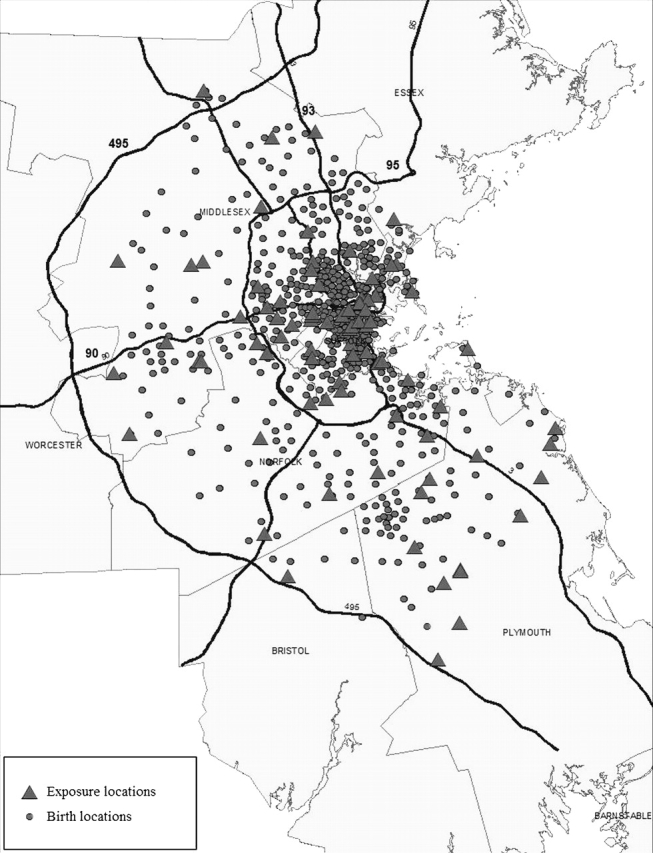
Map of the locations of the residences of the birth weight study subjects and their positioning relative to the 82 exposure monitors.

In this analysis, we first fitted linear regression models for birth weight in grams. In this huge–sample size setting, Bayesian approaches are computationally demanding and thus infeasible to apply in a reasonable amount of time. Accordingly, we use the naive plug-in, exposure simulation, and the RC-OOS approaches to analyze the data. We also applied standard weighted least squares, but relegate reporting of this result to Section B of the supplementary material available at Biostatistics online. Because our health outcome is a pregnancy outcome, we used as our exposure metric 9-month averages of 24-h predicted BC levels corresponding to the gestational period for each birth. We note that, although the timescales of our prediction model (daily) and our exposure covariate (9 months) do not coincide, the use of the estimate to correct the naive plug-in estimator is still valid due to the linear assumption in the validation relationship (4.2). To account for well-known confounding factors of birth weight, we included the following covariates on biologic grounds: maternal age, maternal race, gestational age, amount of cigarette smoking during pregnancy, chronic conditions of the mother or pregnancy, mother having previous preterm birth, mother having previous infant weighing > 4000 g, gender, year of birth, maternal education, Kotelchuck index of adequacy of prenatal care, and census tract (CT) median income. We include education and CT median income to account for both individual as well as contextual effects of socioeconomic status, a well-known important predictor of birth weight, on the outcome.

Table 3 presents the estimated coefficients and estimated 95% CIs for all terms included in the model based on the RC-OOS fit. This approach yields moderate evidence of an association between birth weight and predicted BC concentrations. To put the magnitude of this estimate into perspective, we compare it to the estimated coefficients for other factors well known to affect birth weight. We estimate an interquartile range change in BC (IQR = 0.20 μg/m³) is associated with a decrement in birth weight roughly equivalent to a 10th of the difference between high school and college educated women.

Table 3.

RC-OOS estimates for greater Boston birth weight data

Method	Estimate	SE	95% CI
Predicted BC	– 9.46	4.38	( – 18.05, – 0.88)
Mother's age	6.36	0.20	0(5.97, 6.75)
Gestational age	551.45	6.16	0(539.37, 563.52)
Gestational age squared	– 5.72	0.08	..( – 5.88, – 5.55)
Number of cigarettes	– 28.91	0.84	0( – 30.56, – 27.26)
Number of cigarettes squared	0.69	0.04	0(0.61, 0.78)
Previous infant weighing > 4000	480.10	11.56	0(457.43, 502.77)
Previous preterm	– 242.10	12.82	0( – 267.23, – 216.97)
Maternal condition	– 29.89	3.40	0( – 36.56, – 23.23)
CT median income (1000 K)	0.15	0.04	0(0.07, 0.24)
Maternal education (< 12 years)	8.57	6.74	.( – 4.63, 21.77)
Maternal education (12–16 years)	1.00 (ref)	—	0(—,—)
Maternal education (> 16 years)	16.63	2.52	0(11.70, 21.57)
Race (Caucasian)	1.00 (ref)	—	.(—,—)
Race (African American)	– 131.01	3.64	0( – 138.15, – 123.87)
Race (Asian)	– 192.72	3.99	0( – 200.54, – 184.90)
Race (other)	– 93.15	3.85	( – 100.69, – 85.61).
Sex (male)	132.62	2.06	-0(128.58, 136.66).
Sex (female)	1.00 (ref)	—	.(—,—)
1996	19.37	3.96	0(11.61, 27.14)
1997	16.52	4.36	00(7.97, 25.06)
1998	23.73	3.85	0(16.18, 31.27)
1999	17.02	3.78	00(9.61, 24.43)
2000	10.49	3.77	00(3.09, 17.89)
2001	3.36	3.75	.( – 3.98, 10.70)
2002	1.00 (ref)	—	.(—,—)
Kotelchuck index (inadequate)	– 70.39	4.31	0( – 78.85, – 61.94)
Kotelchuck index (intermediate)	– 51.16	4.36	0( – 59.71, – 42.61)
Kotelchuck index (appropriate)	1.00 (ref)	—	.(—,—)
Kotelchuck index (appropriate +)	– 16.17	2.43	0( – 20.92, – 11.41)

Table 4 presents the results from the 3 different analyses, showing that the relative performance of the various methods follows the patterns suggested by both the analytical results and the simulation studies presented in Sections 5 and 6, respectively. Compared to the naive plug-in approach, exposure simulation grossly attenuates the estimated health effect. Based on the held-out data, our proposed regression calibration correction approach yields ₀ = 0.20 (SE = 0.04) and ₁ = 0.84 (SE = 0.07). Although RC-OOS detects an association between birth weight and estimated BC particle levels at the 95% confidence level whereas the naive approach does not, the magnitudes of these estimates are relatively close in this case, suggesting that the performance of the plug-in approach that simply uses the exposure estimates is not too bad. However, one would not have known this before performing this measurement error correction.

Table 4.

Results for greater Boston birth weight data

Method	Estimate	SE	95% CI
	(in g)
Plug-in	– 7.27	3.78	( − 14.68, 0.14)
Exposure simulation	− 0.48	3.40	( − 7.13, 6.18)
RC-OOS	− 9.46	4.38	( − 18.05, − 0.88)

Because we controlled for a host of well-known confounding factors that explain a large amount of the spatial pattern in birth weights, the regression model assumes independent errors. We checked the appropriateness of this assumption by constructing a semivariogram plot (Waller and Gotway, 2004, Section 8.2) based on the model residuals. This plot (not shown) showed that the semivariance of differences between pairs of residuals is approximately a constant function of distance between each pair, suggesting that the independence assumption is valid for these data.

We reran the above analyses 2 additional times using estimated location-specific BC concentrations during the time periods corresponding to the first trimester and the third trimester of each pregnancy. Interestingly, the effect estimates from the third trimester model were similar in magnitude to those in Table 4, whereas the effect estimates from the first trimester model were all approximately half of those in Table 4. This may occur because the third trimester is the more important period for weight gain of a developing fetus.

Finally, we also ran logistic regression models relating the probability of an infant having a low birth weight for their gestational age to the same exposure predictions used in the linear models for birth weight. As suggested by our simulations in this setting, the differences between the estimates from the different approaches were smaller than those observed in the linear setting, and none of the analyses showed strong evidence of an association between this binary outcome and estimated BC levels (results not shown).

8. DISCUSSION

Taken together, the simulation results suggest that several approaches to analyzing spatially misaligned point data may be appropriate, depending on the amount of spatial heterogeneity in the exposure surface and the amount of data. For moderate sample sizes, a Bayesian approach to estimation is computationally feasible and seems to possess relatively good frequentist properties. The 2-stage Bayesian approach allows one to break the joint model down into its 2 components. Simulation results suggested that this approach approximates the fully Bayesian results quite well. Thus, this 2-stage estimator is attractive whenever either the exposure or health model is complicated, in which case designing well-mixing MCMC algorithms for the full model may be difficult, or when one is interested in running multiple epidemiological models but wants to avoid fitting the exposure model multiple times. Alternatively, one could consider the RC-OOS approach. It is much easier to implement computationally, but is less statistically efficient, than the Bayesian approaches. These 2 features make it more attractive than the Bayesian approaches in large sample settings since the Bayesian approaches can be computationally expensive and the inefficiency of the calibration estimators is not as much of a concern in this setting. The calibration parameters can be precisely estimated, which should improve the MSE compared to that seen in our simulations. Thus, the 2 approaches that work well in all of our simulation settings, the Bayesian and calibration approaches, are complementary in terms of data settings for which each might be preferred.

Our results provide insight regarding existing findings in covariate-response misalignment problems. In a setting where the response and a covariate were misaligned over time, Higgins and others (1997) noted that the plug-in estimator incurred little bias. The unknown smooth trends in the covariate over time were relatively smooth, so these results are the temporal analog of our results based on a spatially smooth surface. Zhu and others (2003) considered Bayesian approaches for spatial data that involve both misalignment and change of support, with interest focusing on relating monitoring data to zip code level disease counts. They noted that a fully Bayesian approach performed well in this setting. Interestingly, these authors also showed via simulation that the exposure simulation approach performed similarly to the fully Bayesian approach, with the estimates of the exposure simulation approach being only slightly biased. Due to the differences between this problem and the one we consider here, there could be multiple reasons for this difference in findings. One possibility is that calculating exposure at the zip code level of aggregation yields relatively smooth exposure surfaces, for which any approach seems to perform adequately.

In short, we used a simple linear model setting to illustrate measurement error issues associated with point-level, spatially misaligned exposure and health data and ran simulations for linear and logistic models. Of course, in practice, more complicated models may be necessary, and future research will focus on extending the methods considered here to such settings. Examples include settings involving health outcomes in complex spatiotemporal models, health effects models exhibiting spatially correlated residuals, and heavy-tailed prediction errors likely to arise for some exposures. One might also consider the impact of different spatial configurations and numbers of exposure monitors and health observations as well as strategies for optimal monitoring design in such settings.

FUNDING

National Institute of Environmental Health Sciences (ES012044 to A.G. and B.A.C., ES009825 to J.S. and B.A.C., ES007142 and ES000002 to C.J.P.); Environmental Protection Agency (R-832416 to J.S. and B.A.C.).

References

- Banerjee S, Carlin BP, Gelfand AE. Hierarchical Modeling and Analysis for Spatial Data. New York: Chapman & Hall; 2004. [Google Scholar]
- Berhane K, Gauderman WJ, Stram DS, Thomas DC. Statistical issues in studies of the long-term effects of air-pollution: the Southern California Children's Health Study. Statistical Science. 2004;19:414–449. [Google Scholar]
- Berry SM, Carroll RJ, Ruppert D. Bayesian smoothing and regression splines for measurement error problems. Journal of the American Statistical Association. 2002;97:160–169. [Google Scholar]
- Carroll RJ, Ruppert D, Stefanski LA. Measurement Error in Nonlinear Models. New York: Chapman & Hall; 1995. [Google Scholar]
- Chib S, Greenberg E. Analysis of multivariate probit models. Biometrika. 1998;85:347–361. [Google Scholar]
- Christensen OF, Roberts GO, Sköld M. Robust Markov chain Monte Carlo methods for spatial generalized linear mixed models. Journal of Computational and Graphical Statistics. 2006;15:1–17. [Google Scholar]
- Cowles MK, Carlin BP. Markov chain Monte Carlo convergence diagnostics: a comparative study. Journal of the American Statistical Association. 1996;91:883–904. [Google Scholar]
- Cressie NAC. Statistics for Spatial Data. New York: John Wiley & Sons; 1993. [Google Scholar]
- De Iorio M, Verzilli CJ. A spatial probit model for fine-scale mapping of disease genes. Genetic Epidemiology. 2007;31:252–260. doi: 10.1002/gepi.20206. [DOI] [PubMed] [Google Scholar]
- Gaudard M, Karson M, Linder E, Sinha D. Bayesian spatial prediction. Environmental and Ecological Statistics. 1999;6:147–171. [Google Scholar]
- Gelman A. Prior distributions for variance parameters in hierarchical models. Bayesian Analysis. 2006;1:515–533. [Google Scholar]
- Gryparis A, Coull BA, Schwartz J, Suh HH. Semiparametric latent variable regression models for spatio-temporal modeling of mobile source particles in the greater Boston area. Journal of the Royal Statistical Society, Series C. 2007;56:183–209. [Google Scholar]
- Higgins KM, Davidian M, Giltinan DM. A two-step approach to measurement error in time-dependent covariates in nonlinear mixed-effects models, with application to IGF-1 pharmacokinetics. Journal of the American Statistical Association. 1997;92:436–448. [Google Scholar]
- Hobert JP, Altman NS, Schofield CL. Analyses of fish species richness with spatial covariate. Journal of the American Statistical Association. 1997;92:846–854. [Google Scholar]
- Kammann EE, Wand MP. Geoadditive models. Journal of the Royal Statistical Society, Series C. 2003;52:1–18. [Google Scholar]
- Kunzli N, Jerrett M, Mack WJ, Beckerman B, LaBree L, Gilliland F, Thomas D, Peters J, Hodis HN. Ambient air pollution and atherosclerosis in Los Angeles. Environmental Health Perspectives. 2005;113:201–206. doi: 10.1289/ehp.7523. [DOI] [PMC free article] [PubMed] [Google Scholar]
- Little RJA. Regression with missing X's. A review. Journal of the American Statistical Association. 1992;87:1227–1237. [Google Scholar]
- Madsen L, Ruppert D, Altman NS. Regression with spatially misaligned data. Environmetrics. 2008;19:453–467. [Google Scholar]
- Maynard D, Coull BA, Gryparis A, Schwartz J. Mortality risk associated with short-term exposure to traffic particles and sulfates. Environmental Health Perspectives. 2007;115:751–755. doi: 10.1289/ehp.9537. [DOI] [PMC free article] [PubMed] [Google Scholar]
- McCullagh P, Nelder JA. Generalized Linear Models. New York: Chapman & Hall; 1989. [Google Scholar]
- Ochi Y, Prentice RL. Likelihood inference in a correlated probit regression model. Biometrika. 1984;71:531–543. [Google Scholar]
- Paciorek CJ. Computational techniques for spatial logistic regression with large dataset3s. Computational Statistics and Data Analysis. 2007;51:3631–3653. doi: 10.1016/j.csda.2006.11.008. [DOI] [PMC free article] [PubMed] [Google Scholar]
- Paciorek C, Yanosky J, Puett R, Laden F, Suh H. Practical large-scale spatio-temporal modeling of particulate matter concentrations. Annals of Applied Statistics. 2008 (in press) [Google Scholar]
- Rougier J. Comment on article by Sans'o et al. Bayesian Analysis. 2008;3:45–56. [Google Scholar]
- Rubin DB. Multiple Imputation for Nonresponse in Surveys. New York: John Wiley & Sons; 1987. [Google Scholar]
- Ruppert D, Wand MP, Carroll RJ. Semiparametric Regression. Cambridge, UK: Cambridge University Press; 2003. [Google Scholar]
- Shaddick G, Wakefield J. Modelling daily multivariate pollutant data at multiple sites. Journal of the Royal Statistical Society, Series C. 2002;51:351–372. [Google Scholar]
- Thoresen M, Laake P. A simulation study of measurement error correction methods in logistic regression. Biometrics. 2000;56:868–872. doi: 10.1111/j.0006-341x.2000.00868.x. [DOI] [PubMed] [Google Scholar]
- Thurston SW, Spiegelman D, Ruppert D. Equivalence of regression calibration methods in main study/external validation study designs. Journal of Statistical Planning and Inference. 2003;113:527–539. [Google Scholar]
- Wakefield J, Shaddick G. Health-exposure modeling and the ecological fallacy. Biostatistics. 2006;7:438–455. doi: 10.1093/biostatistics/kxj017. [DOI] [PubMed] [Google Scholar]
- Waller LA, Gotway CA. Applied Spatial Statistics for Public Health Data. New York: John Wiley & Sons; 2004. [Google Scholar]
- Wand MP. The semipar package reference manual. Technical Report. 2008 Available at http://cranr-project.org/web/packages/SemiPar/SemiPar.pdf. (accessed June 2008) [Google Scholar]
- Yucel RM, Zaslavsky AM. Imputation of binary treatment variables with measurement error in administrative data. Journal of the American Statistical Association. 2005;100:1123–1132. [Google Scholar]
- Zhu L, Carlin BP, Gelfand AE. Hierarchical regression with misaligned spatial data: relating ambient ozone and pediatric asthma ER visits in Atlanta. Environmetrics. 2003;14:537–557. [Google Scholar]
- Zidek J, Shaddick G, White R, Meloche J, Chatfield C. Using a probabilistic model (pCNEM) to estimate personal exposure to air pollution. Environmetrics. 2004;16:481–493. [Google Scholar]
Associated Data
This section collects any data citations, data availability statements, or supplementary materials included in this article.