A Bayesian model for evaluating influenza antiviral efficacy in household studies with asymptomatic infections

Abstract

Antiviral agents are an important component in mitigation/containment strategies for pandemic influenza. However, most research for mitigation/containment strategies relies on the antiviral efficacies evaluated from limited data of clinical trials. Which efficacy measures can be reliably estimated from these studies depends on the trial design, the size of the epidemics, and the statistical methods. We propose a Bayesian framework for modeling the influenza transmission dynamics within households. This Bayesian framework takes into account asymptomatic infections and is able to estimate efficacies with respect to protecting against viral infection, infection with clinical disease, and pathogenicity (the probability of disease given infection). We use the method to reanalyze 2 clinical studies of oseltamivir, an influenza antiviral agent, and compare the results with previous analyses. We found significant prophylactic efficacies in reducing the risk of viral infection and infection with disease but no prophylactic efficacy in reducing pathogenicity. We also found significant therapeutic efficacies in reducing pathogenicity and the risk of infection with disease but no therapeutic efficacy in reducing the risk of viral infection in the contacts.

1. INTRODUCTION

Simulation studies have suggested that antiviral agents such as oseltamivir can be helpful in mitigating potential influenza pandemics (Longini and others, 2005; Ferguson and others, 2005; Halloran and others, 2008). These findings rely on current knowledge about the antiviral agents’ efficacies and characteristics of influenza, such as transmission capacity and natural disease history, obtained from clinical studies in seasonal epidemics. However, the estimability of efficacy measures and the reliability of the efficacy estimates depend on the design of the studies, the size of the epidemics, and the method used. While it is impossible to change the design and scale of existing studies, new statistical methods may provide new insights about antiviral efficacies and characteristics of influenza. In this manuscript, we propose a new approach that makes use of more clinical information than previous methods. We use the approach to reanalyze 2 trials of oseltamivir and compare our findings with published results.

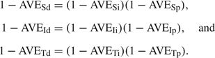
The risk of person-to-person viral transmission depends on the treatment status of both the infective case and the susceptible contact. Let R_uv denote the risk if the treatment status is u for the infective case and v for the susceptible contact, u,v = 0(no),1(yes). Following the notation in Halloran and others (2007), AVE_S = 1 − (R₀₁/R₀₀) measures the antiviral efficacy in reducing susceptibility, AVE_I = 1 − (R₁₀/R₀₀) measures the antiviral efficacy in reducing infectiousness, and AVE_T = 1 − (R₁₁/R₀₀) is called the total efficacy. Depending on the primary end point for analysis, one may use (AVE_Sd, AVE_Id, AVE_Td) for infection with disease (symptomatic) and (AVE_Si, AVE_Ii, AVE_Ti) for infection (symptomatic or asymptomatic). The antiviral efficacy in reducing pathogenicity, the probability of illness given infection, is usually measured by AVE_P. Table 1 summarizes the different antiviral efficacy measures introduced here and in the subsequent sections. A more comprehensive introduction of efficacy measures can be found in Halloran and others (1997).

Table 1.

Definitions of antiviral efficacy measures for different end points, depending on the antiviral treatment status of an infective case and a susceptible contact

Antiviral efficacy	Formula†‡	Interpretation
AVESi	1 – R01/R00	Efficacy in reducing susceptibility to viral infection when the contact is treated.
AVEIi	1 – R10/R00	Efficacy in reducing infectiousness causing viral infection when the case is treated.
AVETi	1 – R11/R00	Total efficacy in reducing risk of viral infection when both the case and the contact are treated.
AVESp	1 – η01/η00	Efficacy in reducing pathogenicity in the contact when the contact is treated.
AVEIp	1 – η10/η00	Efficacy in reducing pathogenicity in the contact when the case is treated.
AVETp	1 – η11/η00	Total efficacy in reducing pathogenicity in the contact when both the case and the contact are treated.
AVEP	1 – η∗1/η∗0	Traditional antiviral efficacy in reducing pathogenicity in the contact when the contact is treated, regardless of the antiviral status in the case.
AVESd		Efficacy in reducing susceptibility to symptomatic infection when the contact is treated.
AVEId		Efficacy in reducing infectiousness causing symptomatic infection when the case is treated.
AVETd		Total efficacy in reducing risk of symptomatic infection when both the case and the contact are treated.

^†R_uv is the risk of viral infection with antiviral status u for the case and v for the contact.

^‡η_uv is the probability of ILI given infection with antiviral status u for the case and v for the contact.

The 2 household-based oseltamivir trials were both conducted in North America and Europe but during different outbreak seasons, one in 1998–1999 and the other in 2000–2001 (details in Table 2). We label the early trial as Osel II and the late one as Osel I. Households were ascertained by the onset of influenza-like illness (ILI) in an index case. Both studies randomized contacts to oseltamivir or placebo at the household level (same treatment in a given household). Osel II did not treat the index cases, whereas Osel I treated the index cases and any contact when symptoms developed, regardless of assigned treatment group. Contacts kept symptom diaries during the follow-up period. Nasal/throat swabs were taken for culture from each participant on day 1 (ascertainment day) and when ILI developed. Blood samples were drawn from each participant on day 1 and at the end of the study to determine the hemagglutination-inhibiting antibody (HI) titer level. Figure 1 illustrates the time frames for the symptom diary and specimen collection.

Table 2.

Data from 2 randomized efficacy trials for oseltamivir. Households with influenza-negative index cases are excluded

	Osel I	Osel II
First analysis	Hayden and others (2004)	Welliver and others (2001)
Households	173	161
Population†	557	564
Treatment for illness	Oseltamivir	None
Duration of medication
Illness treatment	5 days	N/A
Prophylaxis	10 days	7 days
Follow-up (symptom diary)	30 days	7–14 days
Index cases	183	161
Contacts	374	403
Negative swab at baseline	360	391
Control‡	38(6)/171	37(22)/188
Oseltamivir‡	19(2)/189	15(2)/203

^†Three households with index cases < 1 year old are excluded from Osel II, and 132 contacts ≤ 12 years old are excluded from Osel I for comparability between studies.

^‡The number of influenza infections and, in parentheses, the number of influenza infections with ≥ 1 ILI episodes out of influenza-negative contacts at baseline.

Fig. 1.

Time line of symptom diary and specimen collection for Osel I (below) and Osel II (above). Day 1 is the ascertainment day when enrollment of the household occurred, baseline specimens were collected, and symptom diaries started. Day -6 is the earliest day when infection could have occurred by assumption.

Based on the study designs, Osel I mainly provides information about R₁₀ and R₁₁ and Osel II mainly provides information about R₀₀ and R₀₁. In the first analyses of the 2 studies comparing cumulative incidences of symptomatic cases between treatment groups, Welliver and others (2001) reported AVE_Sd and AVE_Si for Osel II and Hayden and others (2004) reported for Osel I. Yang and others (2006) combined the 2 studies to estimate AVE_Sd, AVE_Id, and AVE_Td per daily contact by modeling symptomatic infections. Halloran and others (2007) considered asymptomatic infection in the contacts and obtained estimates for (AVE_Sd, AVE_Id, AVE_Td), (AVE_Si, AVE_Ii, AVE_Ti), and AVE_P from the combined studies. In Halloran and others (2007), the cumulative incidence rates were restricted to days 1–7 to represent secondary attack rates by the index case and the number of secondary asymptomatic infections was imputed based on the assumption that asymptomatic and symptomatic infections are similarly distributed over time. This assumption may be unrealistic if AVE_p is not trivial because the prophylaxis groups would likely have a higher proportion of asymptomatic infections before day 7 compared to the proportion of symptomatic infections.

We propose a Bayesian model taking into account asymptomatic infections to analyze the 2 oseltamivir studies. This model can be extended to general household data with symptom sequence and lab test results available. We also propose a set of efficacy measures for pathogenicity, the estimates of which can be used in conjunction with those for AVE_Si, AVE_Ii, and AVE_Ti to derive estimates for AVE_Sd, AVE_Id, and AVE_Td. In addition, our model estimates the infectivity level over time of an infected person under some parametric assumptions. Bayesian methods have been developed in recent years to model the spread of infectious diseases, but only a few are applicable to influenza in the household setting (O'Neill and others, 2000; Cauchemez and others, 2004; Ferguson and others, 2005). However, none of these methods consider asymptomatic infection.

2. METHODS

2.1. Data structure

Consider a study conducted on H households, household h of size n_h, and observed on a daily basis. We refer to the subject i in household h as subject (h,i). We refer to the enrollment day as the ascertainment day of the index case and the first day of an ILI episode in an individual as the symptom onset day. Without loss of generality, we align all households by setting the ascertainment days as day 1. Let be the stopping day of observation on household h. During the follow-up period, {1,2,…,}, a series of symptom onsets are observed for some contacts, that is, household members who are not index cases. For now, we assume at most one ILI episode can be observed for each subject. Let be the symptom onset day of subject (h,i) and = ∞ if no ILI is observed.

Let y_hi represent all relevant lab test information including specimen collection dates, the tests used, and the test results. Therefore, {,,y_hi:i=1,…,n_h,h=1,…,H} constitute the observed data. The infection dates, denoted by { :i =1, …,n_h, h = 1, …,H}, are the latent data.

2.2. Modeling viral transmission

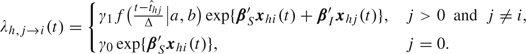
We assume that, starting from day <1, all subjects in household h are exposed to a constant rate of infection, γ₀, from casual contact with people in the local community. In reality, is not observable, but we do not need to, as explained in section 2.4. We speculate that the infectivity (infectiousness) level of an infected person is closely related to the virus-shedding activity and thus the viral load in vivo. Figure 2(a) shows the log viral loads over 7 days in 6 people challenged with an attenuated influenza virus, time 0 being the infection time (Murphy and others, 1980). After enforcing the area under the mean curve to be unity over (0,1), we found that f_Beta(2.08,2.31), obtained by the least squares method, provides a decent fit as shown in Figure 2(b). Let Δ be the duration of the infectious period, assumed known. According to Figure 2(a), Δ = 7 days is a reasonable choice for influenza. Let x_hi(t) indicate the vector of covariates of subject (h,i) on day t, and let β_S and β_I be the effects associated with covariates of the susceptible and infective person. We regard the community as a member of each household and index it by 0. Actual household members in household h are indexed by 1,…,n_h. The covariate-adjusted hazard of influenza infection that an infectious person j imposes on a susceptible person i in household h at time t is

(2.1)

where f(·|a,b) is a beta density function with shape parameters a and b referred to as the relative infectivity curve. The interpretation of γ₁ is the average baseline person-to-person infection rate over the infectious period because 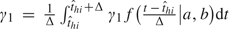. A similar idea of modeling the time-dependent infectiousness level was used in Ferguson and others (2005), where a lognormal curve truncated at a maximum of 10 days was adopted. We assume for now that asymptomatic and symptomatic cases share the same relative infectivity curve and γ₁. The sensitivity of the results to this assumption will be considered in the data analysis. In expression (2.1), the covariate effects are assumed to be the same for exposure from the community as for exposure within household, but different effects could be assumed. The total hazard of influenza infection for a susceptible person (h,i) at time t is then given by λ_hi(t) = ∑_j≠iλ_h,j→i(t), and the probability of escaping influenza infection during day t for person (h,i) is q_hi(t) = exp{ − ∫_{t − 1}^tλ_hi(τ)dτ}.

Fig. 2.

(a) Viral load (log₁₀) over time in 6 subjects challenged with an attenuated influenza at time 0. The solid black line is the mean curve. (b) Fitting the mean viral load (log₁₀) over time in 6 subjects (solid line) with a beta density curve f(a,b) (dashed line). The shape parameters a = 2.08 and b = 2.31 are least squares estimates. The relative infectivity curve estimated by the Bayesian model is f(4.68,4.90) (dotted line).

2.3. Modeling pathogenicity

Let ξ_hi(t) be the probability that subject (h,i) develops ILI given infection on day t. For simplicity, we assume that ξ_hi(t) depends only on antiviral treatment status. When ξ_hi(t) depends on other covariates, the efficacy measures described below will be specific to covariate levels. Let r_hi(t) denote the antiviral treatment status for subject (h,i) on day t, 1 for yes and 0 for no. For the community, r_h0(t) = 0 for all t. Let us consider a simpler scenario first. Suppose there is only a single infectious subject j in household h and disregard the community for now. A possible model for pathogenicity is

(2.2)

Let η_uv = logit ^{− 1}(α₀₀ + vα₀₁ + uα₁₀), the probability of ILI given infection for antiviral status u for the infective and v for the susceptible, u,v = 0,1. Analogous to the definitions of antiviral efficacies in reducing the probability of infection, we can define to denote the antiviral efficacies in reducing pathogenicity for different treatment combinations for the susceptible and the infective (Table 1). It can be shown that the following relationships hold:

(2.3)

When there are multiple infectious sources, including the community, we define an average treatment status over all infectious sources weighted by the daily cumulative hazards, that is, . Other weighting scheme could also be used. Then, we simply replace r_hj(t) in (2.2) with . The underlying assumption of this model is that, while the number of infectious sources affects the probability of infection, exposure to multiple infectious sources does not increase ξ_hi(t) as compared to exposure to only a single infectious source, if the infectious sources receive the same treatment. However, other potential pathogenicity modifiers such as the number of infectious sources could be adjusted for as additional covariates.

Given the infection day and that the infection is symptomatic, we assume that the duration of the incubation period of subject (h,i), −, follows a known discrete distribution Pr(|). Our simulation work suggests that the distributions of the incubation period and the infectious period cannot be estimated together in this model setting (unpublished results).

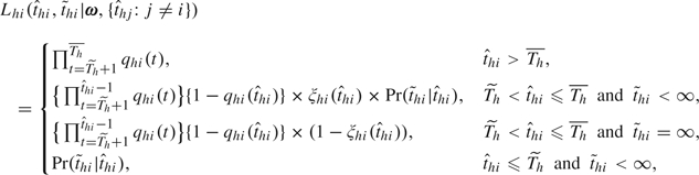
2.4. Joint posterior probability

Define ω = (γ₀,γ₁,β_S,β_I,α₀₀,α₀₁,α₁₀,a,b) as the collection of all parameters to be estimated. Let denote the index case's symptom onset day, and we assume that < ≤ 1. The joint probability concerning influenza infection and the development of ILI for person (h,i) starting from is

(2.4)

where = ∞ indicates that the infection is asymptomatic. The probability histories of escapes, infections, and pathogenicity before +1 are dropped, but the components for the incubation period are retained, to adjust for selection bias as each recruited household has at least one case, that is, the index case (Yang and others, 2006). The selection bias issue can be viewed as a left truncation problem for the number of infections in a household, as 0 number of infection will never occur with this design. Without this adjustment, the estimates of γ₀, α₀₀, α₀₁, and α₁₀ will be biased because index cases have already been infected and developed symptoms without antiviral treatment. Households with lab negative index were also recruited and followed in the oseltamivir studies, but we discard these households for analysis because appropriate adjustment for selection bias for these households is not possible unless the mechanism of generating noninfluenza-caused ILI is also modeled.

Define C(yh_i|) to indicate whether y_hi is compatible with (1, yes; 0, no). For example, if y_hi shows a positive swab on day 1, then C(y_hi|t) = 0 for t ≥ 1 as the infection time should be no later than day 1 to produce a positive baseline lab test. The values of t with C(y_hi|t) = 1 are study specific and depend on how the lab test results indicate the range of possible infection dates, which often involves untestable assumptions. Let π(ω) be the joint prior distribution of the parameters, which is the product of individual prior densities (online supplementary materials available at Biostatistics online). Define the sets .

The joint posterior probability of the parameters and latent infection days is proportional to the full probability of all random quantities:

(2.5)

2.5. Markov chain Monte Carlo sampling

We use Markov chain Monte Carlo sampling to find the joint and marginal posterior distributions for all parameters. The random walk style Metropolis–Hastings algorithm () is used to sample each parameter in ω (sampling scheme in the online supplementary materials available at Biostatistics online). The sampling of the latent infection days is guided by how it will change the probability of all escapes and infections in the household. Denote by Ω_hi the set of candidate infection days for subject (h,i). To differentiate information between symptomatic and asymptomatic infections, we assume that whether a given infection is symptomatic or asymptomatic is determined as the following:

“Set . If Ω_hi is not empty, then person (h,i) is considered a symptomatic case; otherwise, the infection is asymptomatic and .”

To sample an infection day t, we use the conditional probability

(2.6)

3. RESULTS

For the oseltamivir trials, we adjust for age group, in addition to antiviral treatment, in the transmission model as age is known as a modifier for susceptibility (Yang and others, 2006). The 2 age groups are adults ( ≥ 18 years old) and juveniles ( > 12 and  < 18 years). Children contacts ≤ 12 years old were not enrolled in Osel II and are therefore excluded from Osel I for comparability of the analysis combining the studies. Let z_hi denote the age group (1, adult; 0, child). The adjustment for covariates are attained by replacing β_S^′x_hi(t) with r_hi(t)log(θ_Rx) + z_hilog(θ_Age) and β_I^′x_hj(t) with r_hj(t)log(φ_Rx) + z_hjlog(φ_Age) in (2.1). The antiviral efficacies are given by AVE_Si = 1 − θ_Rx and AVE_Ii = 1 − φ_Rx, and we assume multiplicativity such that 1 − AVE_Ti = (1 − AVE_Si)(1 − AVE_Ii). Flat priors are used for all parameters except for the shape parameters of the relative infectivity curve. The details about the prior distributions, the assumptions used to determine C(yh_i|, and thus Ω_hi for these trials are given in the online supplementary materials available at Biostatistics online. We report the posterior medians and the 95% credible sets (CS) for all parameters.

3.1. Primary analysis

The primary results are summarized and compared with previous analyses in Table 3. As γ≈1 − e ^{− γ} when γ is small, the estimates of γ₀ and γ₁ also reflect the daily baseline probability of infection by the community and the average daily baseline person-to-person transmission probability within a household, respectively. Baseline here refers to untreated children. However, due to the exclusion of children ≤ 12 years, the child group in our analysis is actually composed of juveniles. The Bayesian estimates for the baseline infection rates are smaller than the maximum likelihood estimates for the daily probabilities of symptomatic infection among adults in Yang and others (2006), partially because of different assumptions about ILI episodes and lab test results.

Table 3.

Comparison between Bayesian estimates and previous findings. Distribution of the incubation period is {1 day, 0.21; 2 days, 0.58; 3 days, 0.21}. Bayesian estimates are presented as median_{(95% CS)} and the likelihood-based estimates are presented as MLE_{(95% confidence interval)}

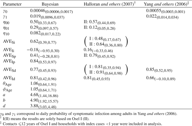The antiviral prophylaxis given to the exposed susceptibles was protective against both influenza infection in general and infection with disease but was not able to reduce pathogenicity in the exposed susceptibles substantially. Our estimate of AVE_Si, 0.62, is close to the estimates in Halloran and others (2007), 0.48 based on Osel I and 0.64 based on Osel II. Our estimate of AVE_Sd, 0.77, is slightly lower than the ones reported in Halloran and others (2007), 0.81 based on Osel I and 0.91 based on Osel II, and in Yang and others (2006), 0.85. Halloran and others (2007) reported 0.56 based on Osel I and 0.79 based on Osel II for the traditional AVE_P which depends only on the antiviral prophylaxis status of the susceptible. In fact, the AVE_P estimate based on Osel II is also an estimate for AVE_Sp based on SARs because all index cases were not treated. Hence, our posterior estimate of AVE_Sp, 0.41, is much lower than previous estimates. The baseline pathogenicity, when neither the infective nor the susceptible are treated, is estimated as 0.57 in Halloran and others (2007), higher than our estimate, 0.50.

In contrast, the therapeutic antiviral treatment for the infectives was not effective in reducing the infectiousness level but was able to reduce pathogenicity and thus able to prevent symptomatic infection in contacts significantly. The estimate of AVE_Ii in Halloran and others (2007), 0.16, is also nonsignificant but has a higher magnitude than our median estimate, − 0.18. Our median estimate for AVE_Id, 0.81, is similar to 0.81 in Halloran and others (2007) and 0.66 in Yang and others (2006).

Age group did not alter either susceptibility or infectiousness, which can be partially explained by the exclusion of young children ( ≤ 12) from both studies in our analyses. To investigate the age effect on pathogenicity, we changed the logistic model for pathogenicity to . The estimate for exp(β), the odds of developing symptomatic disease given influenza infection in adults relative to that in children, is 0.60 (95% CS: 0.18, 2.21), suggesting that infected adults are somewhat less likely to develop ILI as compared to juveniles. The incorporation of age effect in the pathogenicity model will make AVE_Sp, AVE_Ip, AVE_Sd, and AVE_Id age specific.

The posterior medians for the shape parameters of the relative infectivity curve, 4.68 for a and 4.90 for b, differ from the empirical values, 2.08 and 2.31. However, the estimated time of peak infectivity (), 3.30 days (95% CS: 1.93, 4.12), is close to 3.16 obtained from the empirical values. The predicted relative infectivity curve is shown in Figure 2(b) together with the empirical curve. The wide 95% CS for a and b obtained under a relatively strong prior demonstrate the limited information about the relative infectivity curve in the data. If a flat prior is imposed, the estimates for a and b increase substantially to the 10² scale, suggesting that the data do not provide sufficient information about the variability of infectiousness over time. Nevertheless, the estimates for all other parameters remain about the same. For this reason, a and b are assumed known and fixed at their empirical values in all subsequent sensitivity analyses.

We also estimated the generation time, denoted by d, which is defined as the average time it takes for an infective, since his/her own infection time, to infect a susceptible person. The posterior median of d, 3.88, is longer than 2.6 in Ferguson and others (2005) and similar to the serial interval estimates 3–4 days in Viboud and others (2004) and Cowling and others (2009). The serial interval is the length of time between symptom onsets of the 2 sides of transmission. The gap between our estimate of d and that in Ferguson and others (2005) could be due to fact that we use a discrete timescale for infection, and thus the minimum generation time is 1 day.

3.2. Sensitivity analysis

It was speculated that asymptomatic influenza-infected cases are less infectious than symptomatic influenza-infected cases. We performed sensitivity analyses by changing the infectiousness of an asymptomatic infection relative to a symptomatic infection from 1.0 to 0.5 and then to 0.1, and the results are shown in Table 4. When we assume that asymptomatic cases are 50% less infectious than symptomatic cases, we observe an increase in the estimate for γ₁ and decrease for φ_age, with other estimates being fairly stable. When the relative infectiousness level of asymptomatic cases is further reduced, the model tends to explain many infections by increasing community-to-person transmission (γ₀) instead of increasing person-to-person transmission (γ₁), and nearly all estimates become very sensitive except those for AVE_Si and θ_age.

Table 4.

Bayesian estimates by different infectiousness of asymptomatic cases relative to symptomatic cases. The relative infectivity curve is assumed known and set to f_Beta(2.08, 2.31). The distribution of incubation period is {1 day, 0.21; 2 days, 0.58; 3 days, 0.21}. Estimates are presented as median_{(95% CS)}

	Relative infectiousness of asymptomatic infection
	1.0	0.5	0.3	0.2	0.1
γ0	0.00046(0.00006, 0.0017)	0.00063(0.00009, 0.0023)	0.0012	0.0025	0.0062(0.0031, 0.011)
γ1	0.021(0.011, 0.038)	0.037(0.019, 0.067)	0.051	0.054	0.013(0.0003, 0.093)
η00	0.49(0.33, 0.66)	0.48(0.32, 0.65)	0.45	0.38	0.29(0.19, 0.43)
η01	0.30(0.095, 0.58)	0.31(0.10, 0.61)	0.32	0.34	0.35(0.089, 0.80)
η10	0.080(0.018, 0.22)	0.077(0.015, 0.22)	0.076	0.079	0.063(0.0, 1.0)
AVESi	0.61(0.36, 0.78)	0.61(0.35, 0.77)	0.62	0.63	0.54(–0.14, 0.86)
AVEIi	– 0.21(–0.94, 0.29)	– 0.22(–1.0, 0.31)	– 0.29	– 0.29	0.28(–12.62, 0.98)
AVESp	0.38(–0.32, 0.81)	0.35(–0.46, 0.79)	0.26	0.099	– 0.18(–2.06, 0.71)
AVEIp	0.84(0.53, 0.96)	0.83(0.49, 0.97)	0.83	0.80	0.79(–3.57, 1.0)
AVESd	0.77(0.42, 0.93)	0.75(0.38, 0.92)	0.72	0.68	0.50(–0.46, 0.86)
AVEId	0.80(0.38, 0.96)	0.80(0.32, 0.96)	0.78	0.73	0.81(–5.13, 1.0)
θAge	1.07(0.64, 1.87)	1.04(0.64, 1.74)	1.03	1.02	1.0(0.59, 1.77)
ϕAge	1.05(0.64, 1.69)	0.91(0.56, 1.55)	0.81	0.76	1.85(0.25, 38.50)

To investigate the sensitivity of the posterior estimates to the prior distributions, we impose nonflat priors on each parameter, while keeping priors of other parameters flat. The nonflat priors take the form for parameters with domain (0,∞) and for parameters with domain ( − ∞,∞). We set μ, the mode, to the 1st, 10th, 50th, 90th, and 99th percentiles of the posterior distribution based on flat priors, an attempt to make the various extremity levels of the nonflat priors comparable between parameters. The dispersion, σ², is the flat-prior-based posterior variance of the parameter or the log-transformed parameter, depending on the domain. Figure 3 assesses the sensitivity for each individual parameter. The horizontal axis corresponds to the nonflat priors indexed by the percentile, and the vertical axis is for parameters with domain (0,∞) and 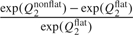for parameters with domain ( − ∞,∞), where Q₂ stands for the posterior median and the superscripts denote the type of the prior distribution. This quantity should be close to 0 if the posterior median for the parameter is insensitive to the choice of the prior. Figure 3 shows that the estimates for γ₀, α₀₁, and α₁₀ are relative more sensitive to the choice of prior distribution than other parameters.

Fig. 3.

Sensitivity of the posterior median to the prior distribution for each parameter, with flat priors for parameters other than the focal one. The new prior mode is set, respectively, to the 1st, 10th, 50th, 90th, and 99th percentiles of the posterior distribution based on the flat prior. The relative infectivity curve is assumed known and set to f_Beta(2.08,2.31).

Additional sensitivity analyses are performed by changing the ILI definition, distribution of the incubation period, the association between infection time and a positive swab (for identifying C(yh_i|)), and the prior distributions, with details given in the supplementary materials available at Biostatistics online. These analyses demonstrate the relative robustness of the estimates for γ₁, AVE_Si (θ_Rx), θ_Age, and φ_Age to a reasonable scope of model assumptions. In addition, reasonable variation in the distribution of the incubation period and the association between infection time and a positive swab have no appreciable impact on the posterior distributions.

4. DISCUSSION

To account for asymptomatic influenza infections, which is the key to the evaluation of the efficacy measures, we developed a Bayesian framework and reanalyzed the combined data from 2 efficacy studies of oseltamivir. As pointed out in Halloran and others (2007), these 2 studies were designed to evaluate the postexposure prophylactic efficacies (AVE_Si, AVE_Sp, and AVE_Sd) of the antiviral agent, not for the therapeutic efficacies (AVE_Ii, AVE_Ip, and AVE_Id). Consequently, combining the 2 studies is necessary for the therapeutic efficacies to be estimable as each study alone does not support such estimation. On the other hand, combining the 2 studies implies a strong assumption: the 2 populations share the same γ₁ and similar pre-epidemic immunity. However, it may not be fruitful to test this assumption before combining the studies. Information about the baseline hazard γ₁ in Osel I is very limited because (1) all symptomatic cases including the index cases were treated with the antiviral and (2) the infection times of asymptomatic cases are too uncertain to provide practically useful information for estimating γ₁. As a result, assuming different γ₁ for the 2 studies will certainly not provide information about therapeutic efficacies and will not necessarily yield more reliable inference about prophylactic efficacies.

The Bayesian estimates for AVE_Si, AVE_Sd, and AVE_Id are close to previously published results, confirming the effectiveness of oseltamivir in reducing transmission of both viral and clinical influenza. The significance of AVE_Sd mainly comes from AVE_Si, whereas the significance of AVE_Id mainly comes from AVE_Ip, which is revealed by analysis for the first time. The Bayesian estimates for AVE_Ii also agree with previous analyses on the absence of the antiviral efficacy in reducing infectiousness.

Additional sensitivity analyses show that estimates for γ₁, AVE_Si, θ_Age, and φ_Age are relatively stable to various model assumptions and prior distributions. Particularly, estimates for all parameters are insensitive to reasonable variation in the distribution of the incubation period and the range of potential infection time that a positive swab can indicate. The sensitivity of the estimates for γ₀, η₀₁ (via α₀₁), and η₁₀ (via α₁₀) to prior distributions reflect to the lack of information in the data for these parameters. The data contain the least information about the shape parameters, a and b, of the relative infectivity curve, however, this uncertainty has very limited influence on the estimation of other parameters. In our unpublished simulation studies that model only symptomatic infections, a and b can be accurately estimated with a sufficient number of cases.

When an efficacy measure is concerned with a postinfection outcome, there may be posttreatment selection bias. In our setting, all efficacy measures except for AVE_Si involve the evaluation of postinfection outcomes and the absence of posttreatment selection bias is implicitly assumed. For vaccine studies, principle stratification can be used to identify the bounds for causal antiviral effects in the presence of posttreatment selection bias (Gilbert and others, 2003; Hudgens and Halloran, 2006). Methods for causal inference in antiviral influenza studies are open to future investigation, for which 2 problems warrant consideration: the violation of the stable unit treatment value assumption and the time dependency of antiviral treatment.

To adjust for selection bias due to case-ascertained enrollment of each household, we truncate the probability on the index case's symptom onset date. Cauchemez and others (2004) used the earliest infection time in the household instead of the index case's symptom onset time as the cut point. However, in our situation, the earliest infection might be asymptomatic, which is not the reason why the household was enrolled. In addition, when the earliest infection time itself is sampled, for example, between 2 candidate days, t₁ and t₂, the conditional probabilities correspond to 2 stochastic processes defined on 2 different domains, (t₁,t₁ + 1,…) versus (t₂,t₂ + 1,…), with one domain nested in the other, likely making the sampling statistically inappropriate.

The symptom diary generally stops at , and consequently, may be right censored (symptomatic) instead of being ∞ (asymptomatic). In (2.4), we ignore the possible right censoring of symptoms after and assume that the infection is asymptomatic. This assumption helps us identify asymptomatic infections with certainty; otherwise, some parameters such as η_uvs may not be identifiable. In studies where asymptomatic infections can be accurately ascertained, for example, through periodic lab tests (instead of symptom driven as in the oseltamivir studies), the right censoring can be appropriately adjusted for.

In future studies, it is recommended that all subjects keep a complete symptom diary up to the day of the last specimen drawn for lab confirmation as in Osel I. While there is a time lag between infection and a 4-fold increase in HI titer level, a complete symptom diary can allow for more comprehensive sensitivity analysis by varying the value of . If it is not possible to obtain a complete symptom diary for each subject in the study population, then households rather than individuals should be sampled to keep a complete symptom diary, so that the sampled households can contribute complete exposure history to the full probability.

Inference can be improved if infection times of asymptomatic cases can be more accurately located. This goal may be attainable by periodic collection of specimens for lab testing at a higher frequency given that the sensitivity and specificity of the test are satisfactory. For example, a recent pilot influenza study was conducted in Hong Kong to evaluate the efficacy of nonpharmaceutical interventions (Cowling and others, 2009), in which nasal and throat swabs were collected every 3 days from each subject. However, the low secondary attack rate (0.06) in this pilot study prevents the use of a complex model like ours for reliable inference about the efficacy measures and the natural history of influenza.

We reiterate that a better designed study is necessary for more reliable evaluation of the effects of therapeutic treatment on the outcomes in exposed contacts. While oseltamivir and other antiviral agents are being stockpiled as a mitigation measure for potential influenza pandemic, we recommend the use of lower values for AVE_Ii in simulation models to evaluate mitigation strategies.

FUNDING

National Institute of Allergy and Infectious Diseases (R01-AI32042); National Institute of General Medical Sciences Models of Infectious Disease Agent Study (U01-GM070749).

References

- Cauchemez S, Carrat F, Viboud C, Valleron AJ, Boëlle PY. A Bayesian MCMC approach to study transmission of influenza: application to household longitudinal data. Statistics in Medicine. 2004;23:3469–3487. doi: 10.1002/sim.1912. [DOI] [PubMed] [Google Scholar]
- Cowling BJ, Fung ROP, Cheng CKY, Fang VJ, Chan KH, Seto WH, Yung R, Chiu B, Lee P, Uyeki TM, Houck PM, Peiris JSM, Leung GM. Preliminary findings of a randomized trial of non-pharmaceutical interventions to prevent influenza transmission in households. Public Library of Science ONE, 2008;3 doi: 10.1371/journal.pone.0002101. e2101. doi:10.137/journal.pone.0002101. [DOI] [PMC free article] [PubMed] [Google Scholar]
- Ferguson NM, Cummings DA, Cauchemez S, Fraser C, Riley S, Meeyai A, Iamsirithaworn S, Burke DS. Strategies for containing an emerging influenza pandemic in SE Asia. Nature. 2005;437:209–214. doi: 10.1038/nature04017. [DOI] [PubMed] [Google Scholar]
- Gilbert PB, Bosch RJ, Hudgens MG. Sensitivity analysis for the assessment of causal vaccine effects on viral load in AIDS vaccine trials. Biometrics. 2003;59:531–541. doi: 10.1111/1541-0420.00063. [DOI] [PubMed] [Google Scholar]
- Halloran ME, Ferguson NM, Eubank S, Longini IM, Cummings DAT, Lewis B, Xu S, Fraser C, Vullikanti A, Germann TC. Modeling targeted layered containment of an influenza pandemic in the United States. Proceedings of the National Academy of Sciences of the United States of America. 2008;105:4639–4644. doi: 10.1073/pnas.0706849105. and others. [DOI] [PMC free article] [PubMed] [Google Scholar]
- Halloran ME, Hayden FG, Yang Y, Longini IM, Monto AS. Antiviral effects on influenza viral transmission and pathogenicity: observations from household-based trials. American Journal of Epidemiology. 2007;165:212–221. doi: 10.1093/aje/kwj362. [DOI] [PubMed] [Google Scholar]
- Halloran ME, Struchiner CJ, Longini IM. Study designs for different efficacy and effectiveness aspects of vaccination. American Journal of Epidemiology. 1997;146:789–803. doi: 10.1093/oxfordjournals.aje.a009196. [DOI] [PubMed] [Google Scholar]
- Hayden FG, Belshe R, Villanueva C, Lanno R, Hughes C, Small I, Dutkowski R, Ward P, Carr J. Management of influenza in households: a prospective, randomized comparison of oseltamivir treatment with or without postexposure prophylaxis. Journal of Infectious Diseases. 2004;189:440–449. doi: 10.1086/381128. [DOI] [PubMed] [Google Scholar]
- Hudgens MG, Halloran ME. Causal vaccine effects on binary postinfection outcomes. Journal of the American Statistical Association. 2006;101:51–64. doi: 10.1198/016214505000000970. [DOI] [PMC free article] [PubMed] [Google Scholar]
- Longini IM, Nizam A, Xu S, Ungchusak K, Hanshaoworakul W, Cummings DAT, Halloran ME. Containing pandemic influenza at the source. Science. 2005;309:1083–1087. doi: 10.1126/science.1115717. [DOI] [PubMed] [Google Scholar]
- Murphy BR, Rennels MB, Douglas RG, Betts RF, Couch RB, Cate TR, Chanock RM, Kendal AP, Maassab HF, Suwanagool S. Evaluation of influenza A/Hong Kong/123/77 (H1N1) ts-1A2 and cold-adapted recombinant viruses in seronegative adult volunteers. Infection and Immunity. 1980;29:348–355. doi: 10.1128/iai.29.2.348-355.1980. and others. [DOI] [PMC free article] [PubMed] [Google Scholar]
- O'Neill P, Balding DJ, Becker NG, Eerola M, Mollison D. Analyses of infectious disease data from household outbreaks by Markov chain Monte Carlo methods. Applied Statistics. 2000;49:517–542. [Google Scholar]
- Viboud C, Boëlle P-Y, Cauchemez S, Lavenu A, Valleron A-J, Flahault A, Carrat F. Risk factors of influenza transmission in households. British Journal of General Practice. 2004;54:684–689. [PMC free article] [PubMed] [Google Scholar]
- Welliver R, Monto AS, Carewicz O, Schattemanet E, Hassman M, Hedrick J, Jackson HC, Huson L, Ward P, Oxford JS. Effectiveness of oseltamivir in preventing influenza in household contacts: a randomized controlled trial. Journal of the American Medical Association. 2001;285:748–754. doi: 10.1001/jama.285.6.748. [DOI] [PubMed] [Google Scholar]
- Yang Y, Longini IM, Halloran ME. Design and evaluation of prophylactic interventions using infectious disease incidence data from close contact groups. Applied Statistics. 2006;55:317–330. doi: 10.1111/j.1467-9876.2006.00539.x. [DOI] [PMC free article] [PubMed] [Google Scholar]
Associated Data
This section collects any data citations, data availability statements, or supplementary materials included in this article.