Glucose Prediction Algorithms from Continuous Monitoring Data: Assessment of Accuracy via Continuous Glucose Error-Grid Analysis

Abstract

Aim

The aim of this article was to use continuous glucose error-grid analysis (CG-EGA) to assess the accuracy of two time-series modeling methodologies recently developed to predict glucose levels ahead of time using continuous glucose monitoring (CGM) data.

Methods

We considered subcutaneous time series of glucose concentration monitored every 3 minutes for 48 hours by the minimally invasive CGM sensor Glucoday® (Menarini Diagnostics, Florence, Italy) in 28 type 1 diabetic volunteers. Two prediction algorithms, based on first-order polynomial and autoregressive (AR) models, respectively, were considered with prediction horizons of 30 and 45 minutes and forgetting factors (ff) of 0.2, 0.5, and 0.8. CG-EGA was used on the predicted profiles to assess their point and dynamic accuracies using original CGM profiles as reference.

Results

Continuous glucose error-grid analysis showed that the accuracy of both prediction algorithms is overall very good and that their performance is similar from a clinical point of view. However, the AR model seems preferable for hypoglycemia prevention. CG-EGA also suggests that, irrespective of the time-series model, the use of ff = 0.8 yields the highest accurate readings in all glucose ranges.

Conclusions

For the first time, CG-EGA is proposed as a tool to assess clinically relevant performance of a prediction method separately at hypoglycemia, euglycemia, and hyperglycemia. In particular, we have shown that CG-EGA can be helpful in comparing different prediction algorithms, as well as in optimizing their parameters.

Background

Noninvasive or minimally invasive sensors have been developed that allow continuous glucose monitoring (CGM) for several days.¹ There is a general agreement that, in the near future, CGM will improve diabetes management by facilitating the appropriate patient reaction to hazardous and potentially life-threatening events, such as hypo- and hyperglycemia. For instance, in order to allow the patient to prevent such events, alerts could be generated on the basis of prediction of glucose concentration ahead of time using past CGM data and appropriate time-series models.

A method (potentially usable in real time) based on modeling of CGM time series was developed² to forecast future glucose levels for a given prediction horizon (PH), e.g., 30 or 45 minutes. The methodology is based on the description of past glucose data through either a first-order polynomial or a first-order autoregressive (AR) model with parameters identified at each sampling time by weighted least squares. Results, obtained with Glucoday® (Menarini Diagnostics, Florence, Italy) time series (3-minute sampling rate) measured in 28 subjects, showed that with both time-series models, glucose can be predicted with a sufficient margin to mitigate critical glycemic events, with a slightly better performance of the AR model.

Computing (in real time) glucose prediction can be useful in improving the mitigation/prevention of hypo- and hyperglycemic events. However, the prediction strategy must be as accurate and reliable (from a clinical point of view) as possible. In this work we propose the assessment of glucose prediction methods by continuous glucose error-grid analysis (CG-EGA). CG-EGA is an approach originally introduced³ to evaluate the clinical accuracy of CGM sensors in terms of both blood glucose (BG) values and BG rate of change. In this article, CG-EGA was used to assess the performance and clinical accuracy of prediction methodologies rather than sensors. In particular, we used CG-EGA to evaluate the clinical accuracy of the two prediction algorithms proposed in Sparacino et al.² This allowed us to evaluate the clinical impact of using predicted glucose levels instead of measured ones in making clinical decisions and in preventing hypo- and hyperglycemic events.

Materials and Methods

Subjects

The database consisted of 28 time series obtained in type 1 diabetic patients with the GlucoDay (Menarini Diagnostics), a minimally invasive sensor composed of a subcutaneous microdialysis probe connected to a light portable apparatus worn with a belt.⁴ Each time series consisted of subcutaneous glucose concentrations determined every 3 minutes for the duration of the study (about 48 hours). This same data set was used in Sparacino et al.²

Prediction Algorithms

For each time series, glucose data are described locally by a time-series model. In Sparacino and co-workers,² to which we refer the reader for details, two possible models were considered: a first-order polynomial and a first-order AR model. In essence, having a fixed model structure, model parameters are fitted at each sampling time, t_N, against past glucose data y_N, y_{N − 1}, y_{N − 2}, …y₁. During parameter estimation, the sample relative to k instants before the actual sampling time (i.e., y_{N − k}) is weighted by the scalar (ff)^k, where the forgetting factor (ff) regulates how past data participate in determination of the time-series model (i.e., the higher the ff, the longer the memory of the past). Then, the fitted model is used to predict the glucose level for a preset PH (e.g., with a sampling interval of 3 minutes, PH = 45 minutes corresponds to a 15-step-ahead prediction). Because Glucoday has no on-board data smoothing or artifact rejection, flat low-pass filtering was applied before applying the prediction algorithm, which removed large spikes occasionally corrupting the time series (for details, see Sparacino et al.²).

Figure 1 displays a representative CGM time series (thin line), together with the corresponding predicted profile (solid line) obtained by the polynomial model with PH = 45 minutes and ff = 0.8 (subject #27). In the predicted profile, the glucose level depicted at time t was calculated PH minutes in advance, at time t–PH. Thus, there is an implicit burn-in interval, which can cause rather large errors in the first hour of prediction. Notably, the predicted profile is more irregular than the measured profile and it is obviously delayed. Sparacino and colleagues² discussed (with several examples) how tuning the parameters of the prediction algorithm, i.e., ff and PH, affects delay and smoothness of the prediction profile.

Figure 1.

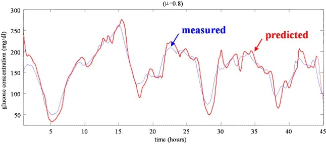
A representative CGM time series (thin line) vs predicted profile (thick line) obtained with the first-order polynomial model with PH = 45 minutes and ff = 0.8 (subject #27).

Continuous Glucose Error-Grid Analysis

An algorithm able to predict glucose fluctuation ahead of time using CGM data can be useful in improving the treatment of diabetes. However, the prediction must be as clinically accurate and reliable as possible. In order to assess the usability of predicted glucose profiles from a clinical point of view, we propose the use of CG-EGA described briefly here. For a detailed description of CG-EGA, we refer the reader to the quoted literature.

CG-EGA was originally designed to evaluate the clinical accuracy of CGM sensors in terms of precision of both BG readings and BG rate of change.³ Augmenting the original Clarke error-grid analysis,⁵ CG-EGA examines temporal characteristics of CGM data. The analysis combines estimates of point and rate precision in a single accuracy assessment presented for each one of three preset BG ranges: hypoglycemia, euglycemia, and hyperglycemia. CG-EGA examines the clinical impact of sensor errors, e.g., what type of clinical outcome might occur if the patient took action based on erroneous CGM feedback about BG levels and rate of change. As pointed out elsewhere,³ BG fluctuations are a continuous process in time. To reflect the temporal characteristics of BG, a new concept of rate-error grid analysis (R-EGA) was introduced, and the traditional Clarke EGA was modified into a new point-error grid analysis (P-EGA). The R-EGA scatter plot is divided into different zones (A through E), which have clinical meaning similar to the original EGA.^5,6 In particular, if a measure falls within the accurate A_R zone, then there is a nearly perfect agreement between reference and sensor glucose rates of change. Zone B_R includes benign errors that do not cause inaccurate clinical interpretation or, if they do, treatment action is unlikely to occur or to result in a negative outcome. Similarly, corresponding zones in the P-EGA are defined depending on the reference rate of BG change. In order to merge R-EGA and P-EGA analysis, CG-EGA computes combined R-EGA and P-EGA accuracy in the three clinically relevant regions of hypoglycemia, euglycemia, and hyperglycemia. This allows the assessment of sensor performance on an error-grid matrix, defined by the extent at which a sensor reading would result in accurate, benign, or wrong treatment.

Assessment of Prediction Algorithms by CG-EGA

The novelty of this article is the use of CG-EGA to assess and compare prediction algorithms. We propose that CG-EGA can be used to evaluate the clinical accuracy of a prediction approach, as well as its impact on decisions to prevent hypo- and hyperglycemic events. Specifically, the 28 predicted profiles were merged in order to generate a single “global” time series (which resulted consisting of 22,961 samples). Then, CG-EGA was used to assess the point and dynamic accuracy of the “global” predicted time series using corresponding measured CGM profiles as reference. In other words, with respect to Kovatchev and co-workers,³ reference BG and sensor BG time series were replaced by measured and predicted time series, respectively. This allowed us to evaluate the clinical impact of using predicted instead of measured glucose levels in diabetes management.

Results

P-EGA and R-EGA

P-EGA and R-EGA scatter plots graphically represent the accuracy of a prediction strategy. Figure 2 shows P-EGA (left) and R-EGA (right) obtained using polynomial (top) and AR (bottom) models with ff = 0.8 and PH = 30 minutes (for clarity, while CG-EGA analysis was carried out on 22,961 samples, results for only 2870 are displayed). P-EGA clearly shows that nearly all the predicted-measured glucose data pairs fall in the A_P zones for both polynomial and AR models, thus confirming that they both provide an accurate proximity between recorded and predicted glucose time series. A very few pairs of points fall in the B_P zone for both time-series models. Less than 10 pairs of points fall in the overcorrection C_P and in the failure to detect D_P zones, especially if the AR model is considered. None fall in the erroneous reading E_P zone. There are no apparent differences between P-EGA plots of polynomial and AR models, with the exception of a wider spread of the former in the B_P zone with BG levels under 150 mg/dl. R-EGA also shows that the majority of the predicted-measured glucose pairs fall in the A_R and B_R zones for both models. This confirms the very good clinical agreement between measured and predicted glucose levels. Occasional pairs of points fall in the C_R zone (i.e., overestimation/underestimation of the measured glucose rate of change). Finally, only a few pairs of points fall in the erroneous D_R and E_R zones where the predicted profile fails to detect significant changes in the measured profile or results in fluctuations opposite to the true rate of change.

Figure 2.

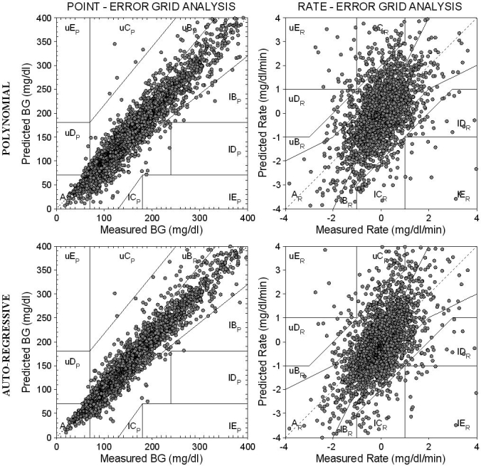
P-EGA (left) and R-EGA (right) obtained for the “global” predicted glucose profile using first-order polynomial (top) and first-order AR (bottom) models with ff = 0.8 and PH = 30 minutes.

Figure 3 shows P-EGA (left) and R-EGA (right) obtained using polynomial (top) and AR (bottom) models, again with ff = 0.8 but with PH = 45 minutes. P-EGA shows that nearly all predicted-measured glucose pairs of points fall in the A_P and B_P zones for both polynomial and AR models, even if a higher PH is considered. As expected, recorded and predicted glucose time series are very close, but P-EGA scatter plots are more spread than those with PH = 30 minutes. A few pairs of points fall in the overcorrection zone C_P, in the failure to detect zone D_P and also in the erroneous zone E_P. No differences are evident between the P-EGA plots obtained by the two models, with the exception of a higher spread of the polynomial model in the B_P zone for BG ≤150 mg/dl. However, these points correspond to prediction errors that do not cause inaccurate clinical interpretation. R-EGA scatter plots (Figure 3, right) show that the majority of the predicted-measured glucose pairs of points fall in the A_R and B_R zones for both models. This confirms the good clinical agreement between measured and predicted glucose levels, even if a longer PH is considered. A few pairs of points fall in the C_R zone. This means that the measured glucose profile would only very rarely lead to overtreatment. Finally, only a few pairs of points fall within D_R and E_R zones.

Figure 3.

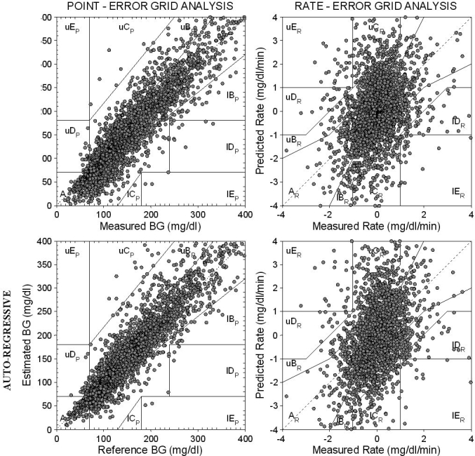
P-EGA (left) and R-EGA (right) obtained for the “global” predicted glucose profile using first-order polynomial (top) and first-order AR (bottom) models with ff = 0.8 and PH = 45 minutes.

The wider spread of the scatter plots obtained with PH = 45 minutes (as compared to PH = 30 minutes), especially in P-EGA, and the presence of a few pairs of points in the erroneous E_P zones are not unexpected because as reported elsewhere,² an increase of PH causes a larger prediction error and wider oscillations in predicted profiles. The same procedure was also applied for ff = 0.2 and 0.5, with both considered PH values (not shown). Similar results were obtained.

CG-EGA Accuracy Table

The CG-EGA computes the so-called error-grid matrix³ in which predicted glucose levels are considered to be clinically accurate when they fall into the A or B zones in both P-EGA and R-EGA. Clinically benign errors are those with acceptable point accuracy (i.e., A or B P-EGA zones) and certain errors in rate accuracy (i.e., C, D, or E R-EGA zones), which are unlikely to lead to negative clinical consequences. Clinically significant errors are those that could lead to a negative clinical action and outcome. Zones considered clinically benign depend on the absolute BG level and are therefore different across the three BG ranges.³

Table 1 presents the CG-EGA error-grid matrix as defined.³ In particular, combined P-EGA and R-EGA results for the “global” predicted glucose profile obtained using either the polynomial or the AR time-series model with ff = 0.8 and PH = 30 minutes are reported in the top and bottom sections, respectively, of Table 1. According to Table 1, the percentage of clinically accurate predictions or predictions resulting in benign errors in the polynomial model are 94.5% at hypoglycemia (91.9% accurate + 2.6% benign), 98.7% at euglycemia (93.1% accurate + 5.6% benign), and 93.9% at hyperglycemia (83.4% accurate + 10.5% benign), thus confirming that performance of the polynomial model is accurate in both normal and critical glucose ranges. The percentage of accurate predictions is significantly higher in hypoglycemia compared to hyperglycemia, which is of particular importance for the forecast of potentially life-threatening events. The highest percentage of accurate readings plus benign errors is obtained at euglycemia, probably because of the smoothness (i.e., small changes in the value of the first time derivative) of the measured time series in the euglycemic range.

Table 1.

Combined P-EGA and R-EGA Results for “Global” Predicted Glucose Profile Obtained Using First-Order Polynomial (Top) and First-Order AR Time-Series (Bottom) Models with ff = 0.8 and PH = 30 Minutes in the Form of CG-EGA Error-Grid Matrix

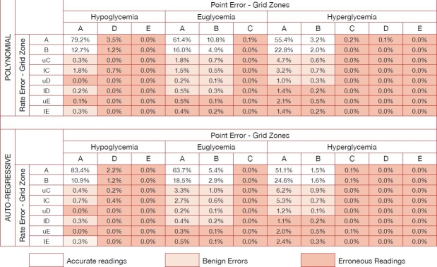Table 1 shows that the percentage of clinically acceptable predictions of the AR model is 96.0% at hypoglycemia (94.3% accurate + 1.7% benign), 99.0% at euglycemia (90.5% accurate + 8.5% benign), and 93.2% at hyperglycemia (78.8% accurate + 14.4% benign). The difference between the percentage of accurate readings plus benign errors obtained at hypo- and hyperglycemia is slightly higher than that with the polynomial model. This is confirmed by the hypoglycemic percentage of accurate predictions, which is now 20% higher than that at hyperglycemia, with a very low percentage of benign errors (i.e., 1.7% at hypoglycemia vs 14.4% at hyperglycemia). This result shows that the predictive strategy based on the first-order AR model is able to achieve excellent accuracy as well. As with the polynomial model, the percentage of accurate readings plus benign errors is highest in the euglycemic range.

Table 2 presents CG-EGA error-grid matrices obtained using either a polynomial or an AR time-series model with variable forgetting factors (ff = 0.8, 0.5, and 0.2) and prediction horizons (PH = 30 and 45 minutes). The polynomial model with ff = 0.8 and PH = 45 minutes shows slightly lower clinically acceptable readings than those obtained with PH = 30 minutes. In particular, the percentage of clinically accurate predictions or predictions resulting in benign errors are 89.3% at hypoglycemia (84.9% accurate + 4.3% benign), 97.4% at euglycemia (86.3% accurate + 11.1% benign), and 91.0% at hyperglycemia (74.8% accurate + 16.2% benign). However, the performance of the polynomial model remains similar in both normal and critical glucose ranges. In contrast, with PH = 30 minutes the percentage of accurate readings plus benign errors is slightly higher at hyperglycemia than at hypoglycemia. As expected, the highest percentage of clinically acceptable predictions is obtained at euglycemia. Similar results are found for the AR model, which results in clinically acceptable predictions of 89.9% at hypoglycemia (86.5% accurate + 3.4% benign), 97.3% at euglycemia (81.7% accurate + 15.6% benign), and 89.6% at hyperglycemia (67.2% accurate + 22.4% benign). The difference between percentage of accurate readings plus benign errors obtained at hypo- and hyperglycemia is very similar to that obtained using the polynomial model, suggesting that the AR model is able to achieve a good accuracy in predicting potentially life-threatening hypoglycemia as well, even if PH increases. Similarly to the polynomial model, the highest percentage of accurate readings plus benign errors is at euglycemia. Finally, as shown in Table 2, results obtained with lower ff values (i.e., ff = 0.2 and 0.5) are less satisfactory.

Table 2.

Percentage of Accurate Readings Plus Benign Errors, Accurate Readings, Benign Errors, and Erroneous Readings for First-Order Polynomial and First-Order AR Predictive Models with ff = 0.8, 0.5, and 0.2 and PH = 30 and 45 Minutes, Respectively

			Hypoglycemia		Euglycemia		Hyperglycemia
			POLYNOMIAL	AR	POLYNOMIAL	AR	POLYNOMIAL	AR
ACCURATE READINGS + BENIGN ERRORS	PH = 30	ff = 0.8	94.5	96.0	98.7	99.0	93.9	93.2
		ff = 0.5	97.2	96.8	98.5	98.3	92.6	91.7
		ff = 0.2	97.5	97.5	97.9	98.0	91.4	90.8
	PH = 45	ff = 0.8	89.3	89.9	97.4	97.3	91.0	89.6
		ff = 0.5	91.4	90.3	96.9	96.5	89.9	87.9
		ff = 0.2	92.3	90.6	97.9	96.1	91.4	87.4
ACCURATE READINGS	PH = 30	ff = 0.8	91.9	94.3	93.1	90.5	83.4	78.8
		ff = 0.5	93.6	93.3	87.8	84.9	75.8	71.6
		ff = 0.2	91.7	92.6	82.8	81.5	69.5	66.9
	PH = 45	ff = 0.8	84.9	86.5	86.3	81.7	74.8	67.2
		ff = 0.5	81.0	82.8	77.3	74.3	64.4	58.5
		ff = 0.2	79.7	81.4	82.8	70.0	69.5	55.0
BENIGN ERRORS	PH = 30	ff = 0.8	2.6	1.7	5.6	8.5	10.5	14.4
		ff = 0.5	3.6	3.5	10.7	13.4	16.8	20.1
		ff = 0.2	5.8	4.9	15.1	16.5	21.9	23.9
	PH = 45	ff = 0.8	4.3	3.4	11.1	15.6	16.2	22.4
		ff = 0.5	10.4	7.5	19.6	22.2	25.5	29.4
		ff = 0.2	12.6	9.2	15.1	26.1	21.9	32.4
ERRONEOUS READINGS	PH = 30	ff = 0.8	5.5	4.0	1.3	1.0	6.1	6.8
		ff = 0.5	2.8	3.2	1.5	1.7	7.4	8.3
		ff = 0.2	2.5	2.5	2.1	2.0	8.6	9.2
	PH = 45	ff = 0.8	10.8	10.1	2.6	2.7	9.0	10.4
		ff = 0.5	8.6	9.7	3.1	3.5	10.1	12.1
		ff = 0.2	7.7	9.4	2.1	3.9	8.6	12.6

These findings suggest that the prediction methodology based on either a first-order polynomial or a first-order AR time-series model² is accurate in both normal and critical glucose ranges. The AR model appears preferable for PH = 30 minutes because it provides a slightly higher percentage of clinically acceptable readings at both hypo- and euglycemia. However, the difference between the two models disappears at PH = 45 minutes. Evaluated via a t test, the difference between results obtained by the two models obtained with different ff and PH values was not significant. Thus, the hypothesis that the two models have an equivalent impact on clinical outcome cannot be rejected statistically. Among the used combinations, the first-order AR model with ff = 0.8 appears preferable because, with an equivalent impact on clinical outcomes, it allows for a slightly higher temporal gain for preventing hypo/hyperglycemic events. Finally, irrespective of the model used, ff = 0.8 is the best among the three tested ff values, yielding the highest percentage of accurate predictions in all three BG ranges.

Conclusions

Previously introduced methods² were implemented to obtain a prediction of glucose fluctuation from past continuous monitoring data 30 or 45 minutes ahead of time. Two different time-series models were used: first-order polynomial and AR models. Results demonstrated that both models allow a satisfactory prediction of future glucose levels, with a temporal gain and a precision depending on two parameters—PH and ff.

The specific goals of this article were (i) to investigate the utility of the CG-EGA for assessing the predictive performance of these two glucose time-series models, (ii) to compare their performance from a clinical point of view, and (iii) to determine ff and PH values that provide the best glucose prediction in terms of clinical accuracy. Tuning of the model parameters and assessment of the clinical accuracy of prediction were based on the CG-EGA,³ which considers both glucose levels and direction and rate of their fluctuations. This is a new application of this analysis, which was originally designed for evaluation of the accuracy of CGM sensors.³

Results obtained on 28 Glucoday time series of Sparacino and colleagues² suggest that the prediction based on either a first-order polynomial or a first- order AR time-series model is accurate in both normal and critical glucose ranges. The AR model seems preferable when a PH of 30 minutes is considered because it provides a slightly higher clinically acceptable percentage of readings at both hypo- and euglycemia. However, this difference disappears when PH = 45 minutes is considered, and the performance of the two models is virtually identical from a clinical point of view. Since the AR model appears to allow for a slightly higher temporal gain in preventing hypo- and hyperglycemic events,² its use is preferable, as already speculated.² Irrespective of the time-series model used, ff = 0.8 yields the highest accurate readings in all the three glycemics for these 3-minute sampled Glucoday data.

Future work on the assessment of glucose prediction algorithms may include an investigation of ways to compare and complement the information coming from CG-EGA with that provided by other metrics, e.g., the quantitative indices of prediction delay and irregularity reported in Sparacino et al.² and the clinical prediction performance index proposed in Facchinetti et al.⁷

Abbreviations

BG

blood glucose

CG-EGA

continuous glucose error-grid analysis

CGM

continuous glucose monitoring

ff

forgetting factor

P-EGA

point-error grid analysis

PH

prediction horizon

R-EGA

rate-error grid analysis

References

- 1.Klonoff DC. Continuous glucose monitoring: roadmap for 21st century diabetes therapy. Diabetes Care. 2005 May;28(5):1231–1239. doi: 10.2337/diacare.28.5.1231. [DOI] [PubMed] [Google Scholar]
- 2.Sparacino G, Zanderigo F, Corazza S, Maran A, Facchinetti A, Cobelli C. Glucose concentration can be predicted ahead in time from continuous glucose monitoring sensor time-series. IEEE Trans Biomed Eng. 2007 May;54(5):931–937. doi: 10.1109/TBME.2006.889774. [DOI] [PubMed] [Google Scholar]
- 3.Kovatchev BP, Gonder-Frederick LA, Cox DJ, Clarke WL. Evaluating the accuracy of continuous glucose-monitoring sensors: continuous glucose-error grid analysis illustrated by TheraSense Freestyle Navigator data. Diabetes Care. 2004 Aug;27(8):1922–1928. doi: 10.2337/diacare.27.8.1922. [DOI] [PubMed] [Google Scholar]
- 4.Maran A, Crepaldi C, Tiengo A, Grassi G, Vitali E, Pagano G, Bistoni S, Calabrese G, Santeusanio F, Leonetti F, Ribaudo M, Di Mario U, Annuzzi G, Genovese S, Riccardi G, Previti M, Cucinotta D, Giorgino F, Bellomo A, Giorgino R, Poscia A, Varalli M. Continuous subcutaneous glucose monitoring in diabetic patients: a multicenter analysis. Diabetes Care. 2002 Feb;25(2):347–352. doi: 10.2337/diacare.25.2.347. [DOI] [PubMed] [Google Scholar]
- 5.Clarke WL, Cox D, Gonder-Frederick LA, Carter W, Pohl SL. Evaluating clinical accuracy of systems for self-monitoring of blood glucose. Diabetes Care. 1987 Sep–Oct;10(5):622–628. doi: 10.2337/diacare.10.5.622. [DOI] [PubMed] [Google Scholar]
- 6.Cox DJ, Gonder-Frederick LA, Kovatchev BP, Julian DM, Clarke WL. Understanding error grid analysis. Diabetes Care. 1997 Jun;20(6):911–912. doi: 10.2337/diacare.20.6.911. [DOI] [PubMed] [Google Scholar]
- 7.Facchinetti A, Sparacino G, Zanderigo F, Cobelli C. Diabetes Technology Meeting. Atlanta, GA: 2006. Nov, Prediction of glucose concentration from CGM data through AR time-series models: role of sampling frequency and other design variables [abstract] [Google Scholar]