SPIDER image processing for single-particle reconstruction of biological macromolecules from electron micrographs

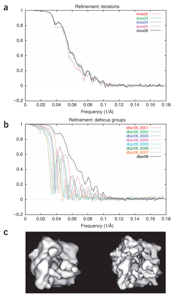
Abstract

This protocol describes the reconstruction of biological molecules from the electron micrographs of single particles. Computation here is performed using the image-processing software SPIDER and can be managed using a graphical user interface, termed the SPIDER Reconstruction Engine. Two approaches are described to obtain an initial reconstruction: random-conical tilt and common lines. Once an existing model is available, reference-based alignment can be used, a procedure that can be iterated. Also described is supervised classification, a method to look for homogeneous subsets when multiple known conformations of the molecule may coexist.

INTRODUCTION

Single-particle reconstruction of molecules from cryo-electron microscopy projections is a field of structure research whose applications are currently proliferating. Following this approach, biological molecules are studied that exist in the specimen not in the form of crystalline aggregates (e.g., as 2D crystals, helical assemblies or icosahedral assemblies), but in the form of single particles lying in random orientations. An intrinsic assumption is that the particle population is homogeneous or that homogeneous subsets can be identified. A limitation of the single-particle reconstruction method is that particles should be of sufficient size such that it allows accurate determination of alignment parameters. Image processing follows various mathematical procedures¹ to determine the orientations of the particles and combine the projection data into a 3D density map of the molecule.

The primary unit of data collection is the ‘electron micrograph’, the image of a field of the specimen recorded either on photographic film or on a charge-coupled device camera. Although photographic film has a much larger information capacity (or useful image field size) than the charge-coupled device camera, it does not lend itself to automated in-line image capture. Each electron micrograph contains 100–1,000 particles, depending on the particle concentration in the buffer and the useful image field size. A reconstruction requires tens of thousands of particles, which means that dozens or hundreds of micrographs need to be collected. For the purpose of image processing, each particle (i.e., particle projection captured in the micrograph) is represented as a 2D array of floating point numbers accompanied by metadata documenting experimental parameters pertaining to the experiment (e.g., defocus) and keeping track of individual measurements such as x/y positions and angles. The collection of particle images associated with a particular reconstruction is referred to as ‘projection data’.

Reconstruction of a 3D density map from EM single-particle projection data requires numerous steps^1,2. Among the mathematical operations to be carried out in the computer are alignment, determination of particle orientation (by random conical technique, common lines or reference to an existing density map), classification, reconstruction and correction of the contrast transfer function (CTF). It was earlier recognized that this kind of multistep processing, often with branching data flow, requires flexible, modular image processing software (SPIDER^3,4, IMAGIC^5,6, EMAN⁷ and XMIPP⁸; for a comprehensive overview, see the image processing software issue of the Journal of Structural Biology⁹). Flexibility is desirable because of the need to explore different image processing and reconstruction strategies. Modularity is called for by the multiple occurrence of identical operations (such as Fourier-transform, cross-correlation, algebraic operations on images) in different contexts. These features of an image processing system make it possible to write programs addressing a new situation without the need to write software on a low level; i.e., the level of FORTRAN, C or C++.

In this article, we present detailed SPIDER protocols on how to proceed from a set of electron micrographs to the reconstruction of a 3D density map. These protocols have the form of scripts (called ‘procedures’ or ‘batch files’) following the syntactic rules of SPIDER. Each of the conceptual steps of single-particle reconstruction (see flowchart in Supplementary Fig. 1 online), such as ‘Alignment’, ‘Data normalization’ or ‘Refinement’, is realized as a sequence of such scripts.

Instead of explicitly running dozens of scripts, these scripts can also be started in the framework of the SPIDER Reconstruction Engine or SPIRE. SPIRE provides a graphical user interface for executing SPIDER scripts, keeping track of the progress of the reconstruction project (see separate section below).

The procedure of this protocol is divided into three sections: (i) random-conical reconstruction; (ii) multiple common lines; and (iii) single-particle reconstruction using the reference-based alignment method. Two approaches are described here to obtain an ab initio structure: random-conical tilt (RCT) and common lines. When an initial 3D model exists, reference-based alignment^10–12 can be used.

Random-conical reconstruction

Random-conical reconstruction is a method proposed by Frank et al.¹³ and implemented by Radermacher et al.^14,15 to produce an initial 3D reconstruction when no a priori knowledge is available on the structure of a macromolecular assembly. This approach is well established for studying single particles^16–18, as many different 2D projections are obtained with only two exposures of the sample to the electron beam.

When considering the set of 2D projections of our particle in Fourier space, they correspond according to the central section theorem to a set of central sections within the 3D Fourier transform of the object, each section being orthogonal to its direction of projection. Therefore, to compute a 3D reconstruction of our object, we need to define the orientation of each central section of our conical tilt series. The conical tilt geometry provides a good sampling of all directions of projections, except in a cone along the z axis. This lack of sampling is responsible for an anisotropic resolution of the 3Dreconstruction along this z axis. However, such limitation can be overcome by merging different set of EM views (e.g., top and side views) or by taking advantage of possible symmetries of the particle.

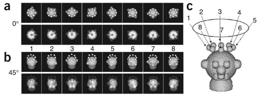
If one considers a set of single particles (little heads in Fig. 1) on an EM grid in one preferred orientation, these particles will produce identical EM views when recording an image with the specimen grid untilted. However, when tilting the specimen grid by a fixed angle, the images collected on the micrograph will correspond to a conical tilt series.

Figure 1.

Geometry for collection of conical tilt data. (a) Surface views (top) and projections (bottom) of a hypothetical 0° view. (b) Surface views (top) and projections (bottom) of a 45° view. (c) Projection directions relative to the object in three dimensions.

In practice, spatial orientations of the 2D projections are defined by Euler angles (http://www.wadsworth.org/spider_doc/spider/docs/euler.html). The RCT 3D reconstruction technique was designed to determine the Euler angles for such experimental data. This protocol comprises four sections:

1. the interactive particle picking on tilted- and untilted-specimen images;

2. 2D image processing of the untilted-specimen images:

   • define Euler angles of all tilted projections and

   • sort images into subsets corresponding to particles with different orientations on the EM grid;

3. computation of 3D reconstructions from selected classes of tilted-specimen images and;

4. correction, if possible, of the ‘missing cone’ artifact, by means of computation of a global 3D reconstruction, by alignment of the individual 3D reconstructions and merging their associated tilted-specimen subsets.

Multiple common lines

A second method to obtain angle assignments for an ab initio reconstruction is by common lines^19,20. The principle is often described under the name of ‘angular reconstitution’ by van Heel²¹, and the procedure below is patterned after a version introduced by Penczek et al.²². Briefly, in accordance with the projection theorem, two 2D projections of a 3D object will intersect along a ‘common line’²³. It follows that data along this line are correlated. By virtue of this relationship, three or more projections, provided they are all not related by rotation around the same axis, can be oriented relative to one another in three dimensions. As raw projection images are too noisy to allow a common-lines alignment, it is necessary to use class averages for this purpose. In our implementation, the class averages are obtained from reference-free alignment and K-means classification. The basic difference between van Heel’s and Penczek’s methods is that van Heel’s proceeds along a sequence of successive angle assignments, one by one, starting from a small set of ‘anchor projections’, whereas the method by Penczek et al. works by optimizing the angle assignments of multiple projections, all at once. An intrinsic problem of common-lines methods is that the handedness of the reconstruction is undecided and that it has to be obtained by a separate experiment or, if the resolution permits, by known chirality of a component.

Reference-based alignment

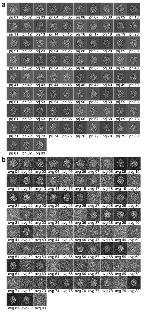
In reference-based alignment, the orientations of the projection data are obtained by comparison to 2D projections of an existing model. A set of 2D reference projections are generated from the 3D reference map, on a coarse angular grid with ~15° spacing, and the corresponding values of alignment parameters (shifts and rotations) are stored. Then, transformations are applied to the particle images according to the values of the alignment parameters. A new model can now be generated, which in turn can be used to refine the alignment parameters iteratively. In the course of angular refinement, iterative methods are applied by matching the experimental projections with those computed from the reconstruction as the angular step size is made smaller and smaller. Thus the experimental particle projections are allowed to ‘settle in’ and find better-fitting angles than available in the initial set of 83 choices. The finally obtained reconstruction is therefore optimally consistent with the data set, provided that no false minimum is reached.

The reference-based alignment protocol comprises two sections:

1. Single-particle reconstruction using the reference-based alignment method^10–12 For the purpose of demonstration, a reconstruction of the Escherichia coli 70S ribosome-elongation factor G (EF-G) complex is generated from10,000 experimental particle images.

   • CTF estimation. The defocus of each micrograph is estimated on the basis of its 2D power spectrum. Then, the micrographs are divided into groups of similar defocus.

   • Particle picking and selection. A particle-picking procedure is used to analyze each micrograph, cutting out of the micrograph small windows, each containing in its center a particle candidate. This procedure is followed by a manual selection process in which the good particle images are identified and the bad ones rejected.

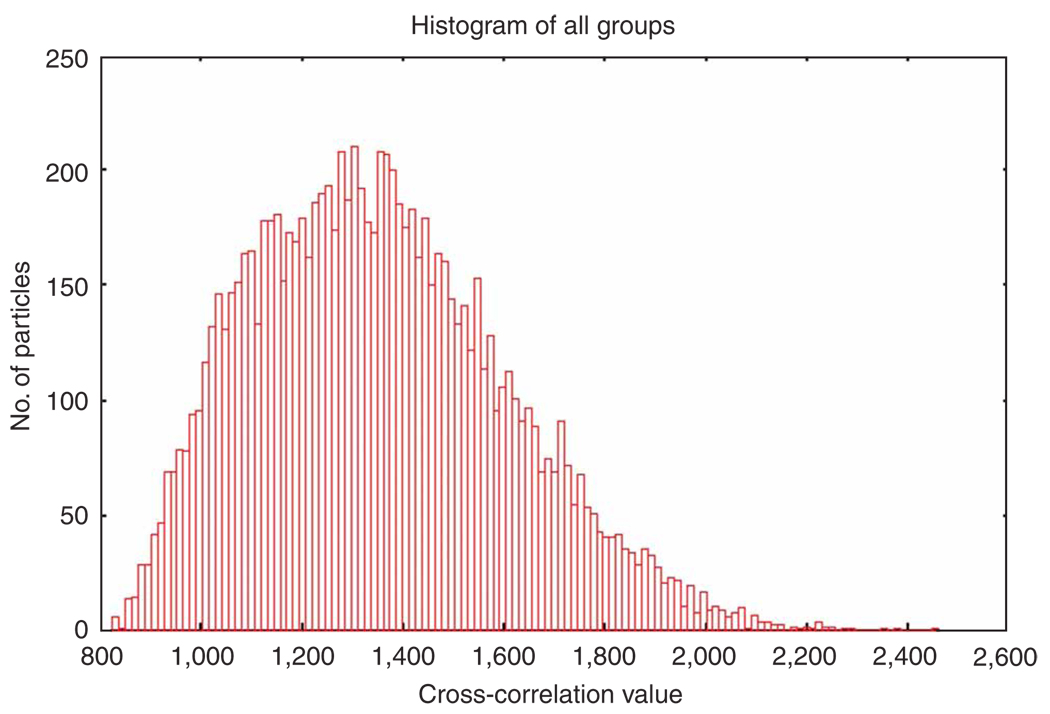
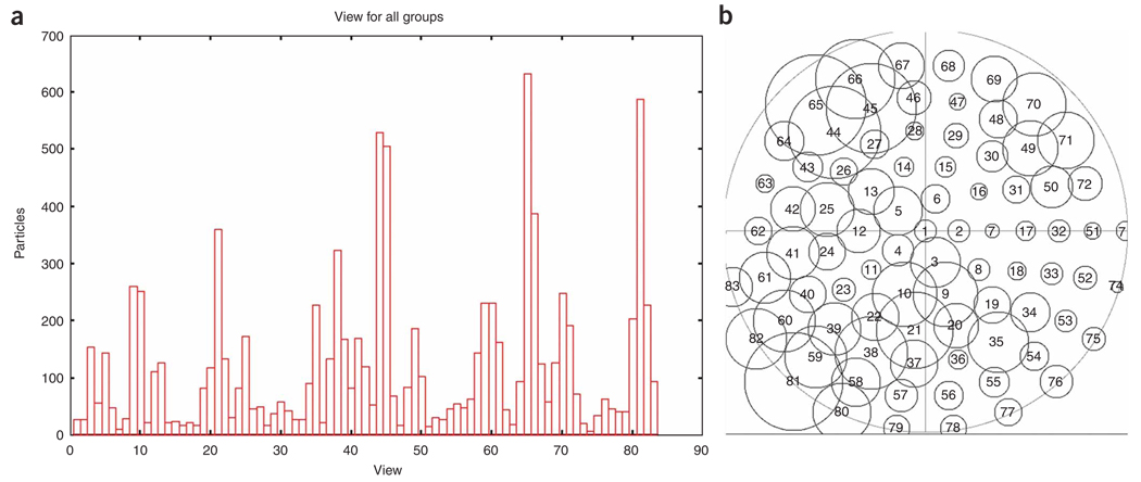
   • Computation of averages. For all projections, all aligned particles of a given reference view are averaged together. Further particle selection is made by selecting a correlation cutoff threshold to reject some inferior particles. The distribution of particles among projections can be displayed.

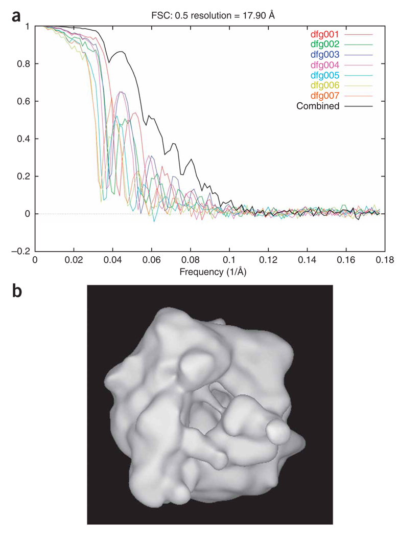
   • Generation of an initial reconstruction. The aligned 2D particle images are used to create an initial 3D reconstruction. To estimate the resolution of the resulting structure, the data are split into two equal sets, and the two resulting reconstructions are compared.

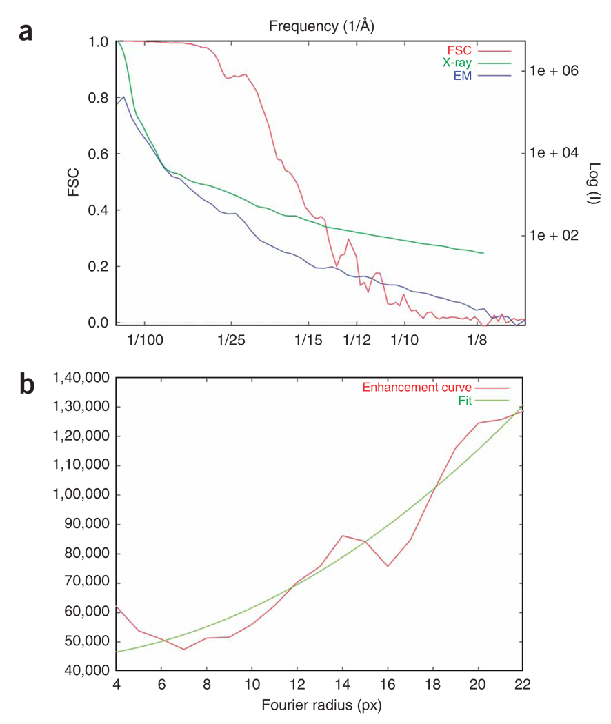
   • Amplitude correction of the EM reconstruction. Fourier amplitudes at higher frequencies are always underrepresented as they are affected by damping factors during data collection (e.g., charging and specimen instability) and image processing (e.g., alignment and interpolation errors). Although the amplitude falloff due to these effects can be approximated as a single Gaussian term, it is difficult to estimate its halfwidth. As exemplified in this protocol, we use a more accurate method to correct the amplitude, by using an empirical (not necessarily Gaussian) function on the basis of a comparison between the radial profiles of the actual Fourier amplitude of the cryo-EM map and the low-angle X-ray solution scattering amplitude, provided such data are available²⁴.

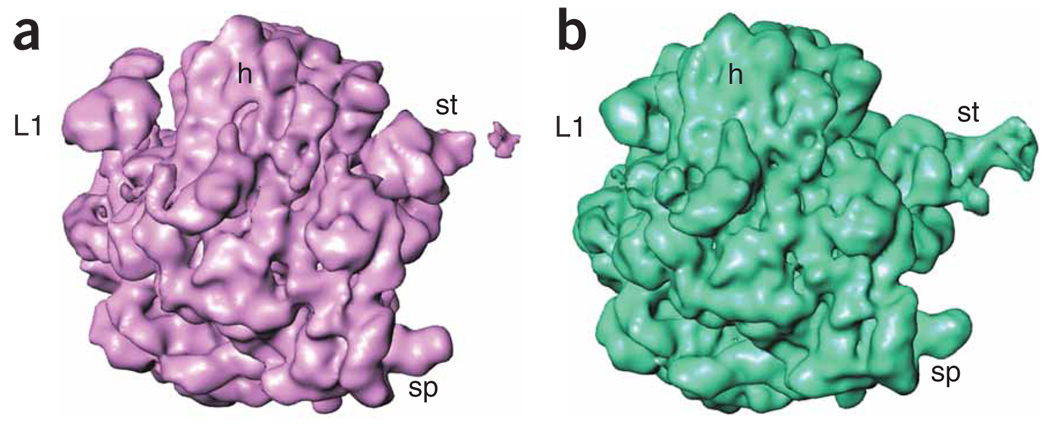
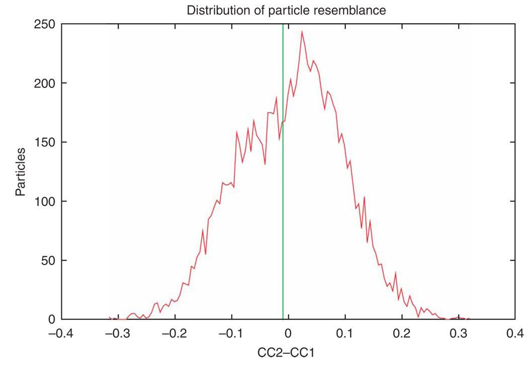
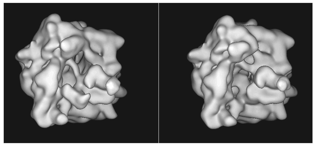
2. Supervised classification. The purpose of supervised classification is to investigate the possible heterogeneity existing in a large cryo-EM data set and sort out the heterogeneous data set on the basis of the resemblance between particle images and two or more reference templates representing different conformational states. For two references, the strategy is as follows: the same reference-based alignment strategy is applied as above, and each particle image is rotationally and translationally aligned with projections of both references. As a result, each particle image bears two cross-correlation coefficients (CC1 and CC2), each associated with a single projection view of one of the two references, respectively. In a case where a particle was assigned to different views for the two references, the view that yielded the higher cross-correlation coefficient is chosen. Taking the cross-correlation coefficient as a measure of resemblance between the reference and the particle image, and forming the difference between the two coefficients, a distribution of the similarity of the particle images with respect to the two references can be derived. According to the similarity distribution, the entire data set can be separated into several subsets^25,26. Finally, by means of the standard single-particle reconstruction method, a 3D density map is computed from each subset.

MATERIALS

EQUIPMENT SETUP

System requirements

The SPIDER image-processing system requires a computer running the Linux, OSX 10 or AIX operating system (OS). (Older releases will also run on SGI Irix.) AMD Opteron or Intel Xeon processors are recommended, as floating-point calculations are dominant. Most compute-intensive operations incorporate open multi-processing (OMP) parallel directives, so SPIDER can make efficient use of multiple processor—multiple core architectures. A 64-bit OS will provide increased speed; however, the program can be run on an older 32-bit OS as well. SPIDER needs at least 256 MB of memory, but 2 GB per core is recommended. We use a SUSE 10+ Linux distribution, but other common distributions work well.

Recompiling requirements

The distribution contains precompiled executables for the following platforms: AMD 32 and 64 bit, Intel 32 bit, OSX 10 on Intel and SGI Itanium. If you wish to recompile SPIDER, both FORTRAN 90 and C compilers are necessary, preferably from the same vendor.

SPIDER software

The SPIDER distribution consists of two separate modules, SPIDER and JWEB. The SPIDER module is written in FORTRAN and is used for mathematical manipulation of images and their contents. The JWEB module is written in Java and is used for visual display and interaction with images created by the SPIDER module or to be used by SPIDER. In addition, there is an older WEB module written in C for use under X-Window system. The WEB display modules will work with most graphics cards on most Linux window managers. Some lower-performance laptop computers may have trouble running the older WEB module under the X-Window system. Operations supported by SPIDER are described in Box 1, and instructions on starting a new SPIDER session are described in Box 2.

BOX 1 | OPERATIONS SUPPORTED.

Following is an overview of operations supported by SPIDER, broken into categories:

File handling and conversion

• Copying, Converting, Stacking and Montaging images, volumes and stacks

Basic image processing

• Contrast enhancement, Arithmetic operations, Rotating, Shifting, Scaling, Windowing, Masking, Thresholding, Filtering, Edge-detection, Histogram analysis and Mirroring

Fourier-space operations

• Fourier transformation, Fourier filtering, Auto- and Cross-Correlation using Fourier theorem, Interpolation

Alignment

• Rotational, Shift, Reference-based and Reference-free alignments

Statistical analysis

• Multivariate statistical analysis, Classification of Image sets, Center of gravity, Variance map

Three-dimensional reconstruction

• Weighted back-projection, ART, SIRT

Resolution determination

• Fourier shell correlation, Differential phase residual, SSNR

Contrast transfer function

• CTF determination, CTF correction through Wiener filter

Graphical representations

• Contouring, Surface shading, Cluster analysis and Graphing

Scripting and flow control

• DO-loops, IF statements, GO TO statements, Variable definition

Document file operations for handling numerical data

• Store, Retrieve, Sort and Process numerical results in SPIDER Document file format

BOX 2 | STARTING A SPIDER SESSION.

To start a SPIDER session, type

spider dat

(where ‘dat’ is understood as the three-letter extension for data files to be accessed in this session).

To run a script, e.g., myscript.bat, type

spider bat/dat @myscript

(i.e., ‘bat’ is the file name extension of the script file, ‘dat’ is the file name extension of the data file, and the name of the file containing the script must be preceded by ‘@’).

Usage

SPIDER operations are usually invoked with two- or three-letter commands, e.g., ‘AP’ or ‘DOC’. Each operation then solicits relevant input and output file names and any necessary input parameters. Many SPIDER operations work on both images (2D arrays) and volumes (3D arrays). A few operations can process a whole image stack within a single operation. SPIDER can be run as an interactive program with immediate access to the results of any operation. SPIDER also contains a set of scripting operations so that it can be programmed and used in a procedural mode. These scripting operations include flow control using ‘IF’ and ‘DO’, modeled on similar FORTRAN commands. In addition, SPIDER contains string variables and floating point variables and a mechanismfor substituting numerical values into strings for creating specific file names, consecutively numbered file names, etc. The various operations can be placed in a procedure or batch file, script files that can be read and interpreted by SPIDER. Sets of partially nested procedures can be written and utilized for the control of complex tasks such as reference-based alignment of projections.

Storage and processing requirements of images in SPIDER

Images and volumes are stored in SPIDER image file format. There is a variable-length header that carries image dimensions, image format and some statistical information. Optionally, it may contain Eulerian angles if applicable, and other pertinent information unique to the image. The image density data are stored in column, row and slice order as IEEE 32-bit floating-point numbers. An image/volume stack format is also available, which has an overall stack header, similar to the image header, followed by a stack of images/volumes in the above format. Images, volumes and stacks can be stored in an internal memory buffer for the duration of a SPIDER session, thereby increasing the access speed. Many of the computationally intensive operations in SPIDER contain OpenMP code for use on shared-memory computers. This capability is available on multicore and multiprocessor Linux and Unix systems supported by SPIDER. Additionally, a few of the compute-intensive image-alignment and back-projection operations have been parallelized for use on message passing interface (MPI) with proper compilation.

Requirements for Fourier transforms

As many of the imaging operations in SPIDER make extensive use of Fourier-space calculations, SPIDER is normally linked with the FFTW (‘The Fastest Fourier Transform in the West’²⁷) C subroutine library for computing discrete Fourier transforms.

Graphical user interface

There is a graphical user interface called WEB for interactive visualization and manipulation of SPIDER images and reconstructions. WEB is available in two versions: (i) ordinary WEB, written in ‘C’, with a point-and-click GUI, and running under the X-Window system; (ii) JWEB, written in Java and running on both Linux and Windows platforms (Box 3 and Box 4).

BOX 3 | WEB OPERATIONS.

WEB operations include the following:

• Displaying images, galleries of images or slices of volumes

• Image contrast enhancement

• Image filtering

• Displaying image histograms

• Windowing (or boxing) subimages from micrographs

• Simultaneous windowing of subimages from two micrographs for random-conical reconstruction

• Density profiling across an image

• Interactive masking

• Power spectrum display

• Image contouring

• Annotation of images

• Recording x/y locations and corresponding densities in images

• Display of correspondence analysis factor maps

• Creating classification dendrograms

• Surface rendering of volumes

BOX 4 | PARALLEL COMPUTING.

Most of the time-consuming operations in single-particle reconstruction can easily be performed in parallel, as there are few cross-dependencies in the processing. Images can be partitioned into groups and distributed among different computers for simultaneous parallel operation. In our examples, the groups are conveniently associated with different defocus levels, but other groupings are also possible. SPIDER includes ‘PubSub’, a Perl script that acts to distribute tasks to be run in parallel on a distributed cluster of computers or within a single cluster. The user places his SPIDER jobs in a shared PubSub queue. Each of the subscriber machines can take jobs from the queue. The use of PubSub is an simple alternative to the use of MPI for parallel operation but, unlike MPI, it can easily utiltize clusters or groups of disparate computers.

SPIRE: the SPIDER reconstruction engine

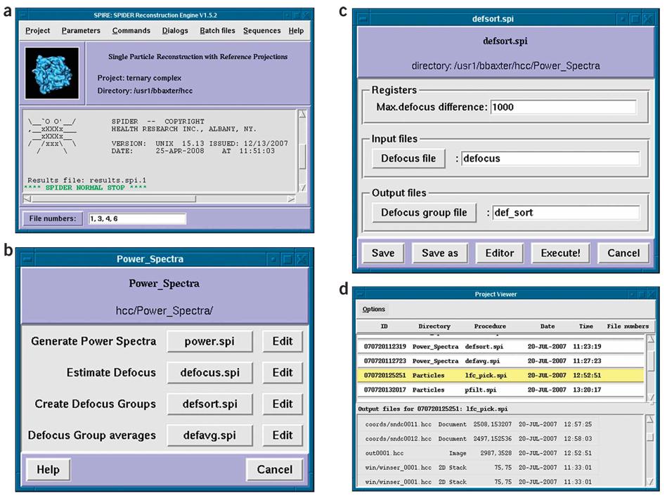
SPIRE²⁸ lets a user run SPIDER batch files in a graphical user interface (Fig. 2a). SPIRE keeps track of procedures and the output files they generate, with a handy interface for viewing all project files. It also provides a convenient environment for testing and debugging batch files. Other features include tools for handling file numbers and project-wide parameters, the ability to save a project in HTML format and a means of accessing external databases. (See the online documentation at http://www.wadsworth.org/spider_doc/spider/docs/spire/index.html for information on downloading and installing SPIRE.)

Figure 2.

SPIRE. (a) SPIRE’s main window. (b) Dialog window with batch-file buttons. (c) The batch file form graphically presents the header values. (d) The Project Viewer.

Projects and dialogs

SPIRE is organized around projects. A project typically consists of an input data set of electron micrographs, the batch files that process the data to produce the result (usually a 3D density map) and numerous intermediate data files. SPIRE projects are organized by project templates called configurations, which indicate the location of the source batch files, the directory structure of a project and how to present the project to the user.

The graphical interface is organized around dialogs (Fig. 2b), which allow the user to launch SPIDER batch files from buttons. With these dialogs, a large number of project batch files can be organized into a few conceptually related units such as particle picking, alignment and power spectrum determination.

Batch files can be executed in SPIDER by pressing the button with the batch file’s name. The input and output files of a batch file can be specified by clicking its accompanying Edit button, which opens a batch file form (see below). The appearance of dialogs is specified by the configuration file, and can be changed in the SPIRE’s Configuration Editor (see below).

Configuration files

SPIRE configuration files are text files, using XML tags to organize their contents, that describe a set of frequently used batch files for various types of projects, such as single-particle reconstruction or tomography. The selected configuration tells SPIRE where to find the source batch files in the user’s file system and where they should be copied to in the working directory of the project. In addition to indicating a project’s directory structure and the location of batch files, the configuration file also specifies how the GUI should present dialogs to the user. There is a Configuration Editor (under the Commands menu), which allows one to change configurations or create new ones.

Starting a new project

In the Projects menu, select New. Fill in the blanks in the presented form; most will have default values. The project file is used to keep track of all batch files run in the course of a project. The project file is a database file created with Python’s shelve module. The configuration file menu provides a list of available configurations, including templates for single-particle reconstruction and tomographic reconstruction, as well as some simple tutorial configurations for familiarizing oneself with SPIRE. Select a configuration for the type of project you wish to carry out. Click OK and SPIRE will create the project subdirectories and copy the batch files from the general repository into the local subdirectories. This way you have your own local copies of the batch files, which can be edited to suit your needs. Once a project has been set up in SPIRE, the batch files may be accessed through the Dialog and Batch file menus. Each dialog lists the batch files that constitute a conceptual unit in the processing pathway. Within each dialog, the batch files appear in the order in which they are typically run.

Editing and running SPIDER batch files

SPIRE requires that batch files have a specific header, containing all registers and file name variables, each with a brief comment. (See a detailed description of the header at http://www.wadsworth.org/spider_doc/spider/docs/spire/wellformed.html.) Clicking a batch file’s Edit button causes SPIRE to read the batch file header and present it to the user in a graphical form (Fig. 2c). Each variable in the header has an entry box, which uses the comment as the label; labels for file names are actually browse buttons that let one search for a file.

The batch file form shows only the default register values, input files and output files that are declared in the header. If you wish to make changes to the processing code outside of the header, click the Editor button to open up the batch file in a text editor. After making the desired changes to the form, clicking Save will write the changes to the local batch file.

A batch file can be run in SPIDER by clicking its button in the dialog. The system command thus executed appears in SPIRE’s main window, along with standard output and any error messages from SPIDER. If SPIDER terminates successfully, SPIRE reads an output file created by SPIDER to see what new files were created and adds the file names to the project file. If there is an error, SPIRE displays the last few lines of SPIDER’s Results file, which usually indicates the source of the error. The current status of the project may be viewed under the Commands menu, View project, which opens the Project Viewer (Fig. 2d).

In its upper panel, the Project Viewer displays all batch files that have completed successfully. Each one has a unique run ID number, the local directory in which it was run, the date and time of execution and, if applicable, the file numbers utilized. Clicking on a batch file displays the files it created in the lower panel. Clicking on an output file displays the files contents: images are viewed in JWEB (see section on SPIDER implementation), whereas document files are viewed in a text editor.

Other features

File numbering

For listing many—perhaps nonconsecutively—numbered file names, some batch files use a SPIDER document file called filenums. SPIRE recognizes this file name and lets the user create it on the fly through the File numbers entry box in the lower left corner of the main window (Fig. 2a). File numbers may be separated either by commas (for explicit, exhaustive specification) or by hyphens (for any stretch of consecutive numbers). It is sometimes helpful to test a batch file with one numbered file after another; this is easy to do with the SPIRE interface. The File numbers label also acts as a browse button for loading file numbers from a document file to use as file numbers in SPIRE.

Parameters

Another common document file is the params file, which contains project-wide parameters that are used in many batch files (such as pixel size or EM acceleration voltage). SPIRE can read this file also and present it graphically. In contrast to the manual procedure of editing register values separately in each batch file, the mechanism of storing parameters in such a centralized location can greatly reduce errors.

The default file names of both the parameter and file numbering files can be changed in the Options section (Commands menu, select Options, then System).

External database

If your laboratory already has a database for reconstruction projects, SPIRE can connect to this external database to obtain or upload project information. This generally occurs at the beginning and end of a reconstruction project. At the start of a project, SPIRE can download some project parameters (e.g., voltage, magnification, scanning resolution) from the database. At the end of a project, results (such as resolution curves, density maps, etc.) can be uploaded into the database. SPIRE provides an application interface, which is a specification of the types of methods it uses to communicate with an external database. The SPIRE distribution contains example code for an example project database in MySQL. See the SPIRE documentation for details about connecting to other databases.

Save a project as HTML

At the end of a project, you can save the contents of the Project Viewer as a set of Web pages (under the Project menu, select Save as html), which lists batch files and their output files in HTML format. This documentation can be saved with the project results, providing a quick index of all batch files that were executed.

Sequences

SPIRE has a convention, called sequences, which allows you to execute any number of batch files with a single button click. A sequence is simply a list of batch files, which is understood to be executed in the order listed. If there is an error, the sequence halts execution. The Sequence menu has items for creating, editing and running sequences.

DATA-SET DESCRIPTIONS

Random-conical reconstruction

Normally, several pairs of micrographs are required to collect enough data for computing a good 3D reconstruction (usually 2,000–3,000 tilted- and untilted-specimen particle images). However, for the clarity of demonstration, we preferred to create a synthetic pair of tilted- and untilted-specimen micrographs. For this purpose, we took from the Macromolecular Structural Database (http://www.ebi.ac.uk/msd-srv/emsearch/) the 3D map of a large macromolecular assembly, the giant hemoglobin from common earthworm Lumbricus terrestris (MSD code: 1078; http://www.ebi.ac.uk/msd-srv/emsearch/atlas/1078_summary.html). This reconstruction was originally obtained at a resolution of 14.9 Å from a set of 16 micrographs, recorded on a JEOL 2010F electron microscope, using an acceleration voltage of 200 kV, a magnification of ×66,489 and defoci ranging from 1,300 to 3,200 nm. These raw data were digitized on a rotating-drum Optronics microdensitometer, with a scanning step and aperture size corresponding to a pixel of 2.5 Å × 2.5 Å on the specimen²⁹.

Multiple common lines

Phantom data used here were generated from the outputs of supervised classification below. A total of 5,000 projections was computed from each of the two reconstructions (as discussed in Step 118 of PROCEDURE), for a total of 10,000 particles. Performance of these procedures is improved when the distribution of orientations is more uniform. Thus, phantom data were used here instead of real data for illustrative purposes.

Reference-based alignment

The cryo-EM data set used in this procedure are translocational ribosomal complexes: 70S●tRNA^fMet●fMet-Ile-tRNA^Ile●EF-G●GDPNP (E. coli ribosome + deacylated P-site tRNA + A-site tRNA with dipeptide + EF-G + GDPNP (a nonhydrolyzable GTP-analog))³⁰. The pretranslocational complex 70S●tRNA^fMet●fMet-Ile-tRNA^Ile was prepared in a highly efficient in vitro system. Subsequent addition of EF-G and GDPNP defines a translocational state that is before the GTP hydrolysis. The solution sample with a final concentration of 32 nM was applied to cryo-EM grids at 4 °C. The micrographs were recorded on the FEI Tecnai F20 electronmicroscope at 200 kV with a calibrated magnification of 49,650, under low-dose conditions. Micrographs were digitized on a Zeiss Imaging scanner (Z/I Imaging) with a step size of 14 µm, corresponding to a pixel size of 2.82 Å on the object scale. A total of 10,000 particles (out of the original 91,114) are used for demonstration in this protocol, with defocus ranging from 2 to 3.5 µm.

PROCEDURE

Random-conical reconstruction

• 1Getting started. First, unpackage the archive randomconical.tar.

  tar -xvf randomconical.tar

  cd Randomconical

  There should be six subdirectories present: hbl/, micrographs/, doc/, images/, r2d/ and r3d/. Those interested to know how the pair of phantom micrographs was created can check batch file b01.mkd. The barrel-shaped six-fold symmetric molecule, which exists in 76 copies, occurs in four orientations on the ’grid’: (1) top view, seen along the 6-fold axis; (2) and (3) side views related to each other by a 30-degree rotation of the molecule around the 6-fold axis; and (4) an intermediate view created by tilting the molecule from the top view position toward the side view. These two micrographs simulate what one would get when observing the same area of a cryo-EM grid with the specimen holder respectively tilted by −45° (tilted-specimen image named rawmic001.hbl) and by 0° (untilted-specimen image named rawmic002.hbl).

• 2Starting SPIRE (optional). To start a new SPIRE project, type spire &. Under Project, select New. Enter a project title and data extension hbl in the appropriate fields. Under Configuration file, browse the directory hbl/ and select RandomConical.xml. The project directory should be the current directory, Randomconical/; the default may be Randomconical/hbl/. Uncheck the box Create directories and load batch files. Do not create a params file, as the parameters used in the batch files below will be self-contained. Going to the Dialogs pull-down menu and selecting batch directory will open a window that contains all of the batch files that will be used here.
• 3Interactive particle picking, using JWEB (Steps 3–13). The two micrographs, in raw 8-byte format (rawmic001.hbl and rawmic002.hbl) in the subdirectory micrographs, will be converted into the REAL*4 SPIDER format. If not using SPIRE, go to the hbl/ subdirectory and then type the command:

  spider fed/hbl b00

  If using SPIRE, click on the button b00.fed. This batch file reads the 8-byte format (rawmic001.hbl and rawmic002.hbl) and converts them into the SPIDER format (mic001.hbl and mic002.hbl). This same batch file also rescales the densities between values of 0 and 1.

• 4JWEB can be used to perform interactive particle picking. For this, the program will be first used to display the two micrographs mic002.hbl and mic003.hbl. Open JWEB by typing at the console jweb &. A main window will appear.
• 5To fit the micrographs on the screen in their entirety, we will set JWEB to reduce images. To do so, in the main JWEB window, go to Options→Settings. Under Resize, click the radio button for Small, and drag the slidebar to, say, 2.0, and click OK.
• 6To open the micrographs, go to File→Open→Image Series, and in the micrographs directory, select mic002.hbl and mic003.hbl. A new window will pop up. Click on the tab labeled Marker-Tilt Pair (Supplementary Fig. 2 online).

  Depending on whether you use one pair of micrographs or several, you can start the numbering of your particles at different values. Here, we set the marker file number equal to 1.

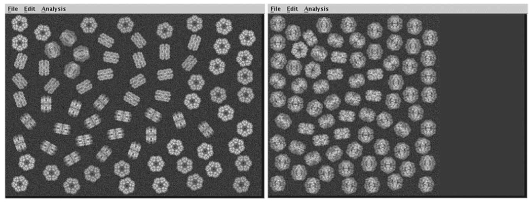
• 7Now, click Show/Edit Marker. The pair of micrographs will pop up (Fig. 3). You will now select one particle within the left-hand side of the screen by putting the arrow on the center of the particle and clicking the mouse. Then you need to select the corresponding particle within the right-hand side of the screen. Identifying constellations of particles in recognizable arrangements will help find the corresponding particle in the tilted image.

  Repeat this pairwise selection for at least four or five particles, as far apart in the micrographs as possible.

• 8Once a large enough area is covered from the first few selected particles, the tilt angle (theta) can be estimated by the program. First, click on Save Marker Files and Determine Theta. The latter step will determine the magnitude of the tilt angle between the untilted and tilted micrographs. Then, click on Fit Angles. The in-plane direction of the tilt axis in the untilted-and tilted-specimen EM fields (phi and gamma) can also be computed at this time (Supplementary Fig. 3 online). By convention, if phi and gamma are close to 0° or 180°, this means that the direction of the tilt axis is close to the y axis of our images on screen. Now, click on Draw Fitted Locations, which will slightly adjust the picked coordinates on the screen. Next, click on Save Angles to save the fitted angles to a file (called dcb001.hbl).

  From now on, the relative orientations of two micrographs are known, so JWEB can help you for the pairwise particle picking. Hence, once you pick the untilted-specimen particle on one side of the screen, the cursor will automatically appear on the other side of the screen on the corresponding tilted-specimen image. You might have to correct the position slightly before clicking on the center of this second particle, but it should be close.

• 9For this tutorial, you will need to select all the particles present on your screen before proceeding. You should get 76 pairs of particles; otherwise, you have missed some.
• 10Once you have finished picking pairs, refine the angles by repeating the sequence above: Save Marker Files, Determine Theta, Fit Angles, Draw Fitted Locations, Save Angles.
• 11To exit JWEB, in the main window, go to File→Exit.
• 12
  All results of your selection are kept in the following document files:

  • dcu001.hbl doc file containing the coordinates of untilted-specimen images
  • dct001.hbl doc file containing the coordinates of tilted-specimen images
  • dcb001.hbl doc file containing the results of the angular determination.

  You can look at the content of these files by typing:

  more dcu001.hbl

  The document file dcu001.hbl contains the coordinates:

  ; hbl/hbl dcu001.hbl Tue Feb 13 16:49:44 2001
  0001	6	1	568	288	284	144	1
  0002	6	2	62	44	31	22	1
  0003	6	3	96	644	48	322	1
  [ . . . ]
  0074	6	74	1012	734	506	367	1
  0075	6	75	812	722	406	361	1
  0076	6	76	914	346	457	173	1
  		IMAGE#	X_COORD	Y_COORD	X_COORD	Y_COORD
  			FULL_SIZE	FULL_SIZE	REDUCED	REDUCED

• 13
  At this stage, you need to move these document files to the subdirectory doc/. The initial locations will be the directory from which JWEB was started, most likely hbl/, micrographs/ or the top-level directory. To move the files from, e.g., hbl/, type the following commands:

  mv dcu001.hbl ../doc/.mv dcu001.hbl ../doc/.mv dcb001.hbl ../doc/.

  
• 14Windowing of isolated particles in individual images (Steps 14–17). Examine the batch files b01.fed and b02.fed, which will be used for the windowing of the two micrographs. These batch files read the document files (dcu001.hbl and dct001.hbl) from the interactive particle selection and create images of 100×100 pixels, written in subdirectory images/. The tilted-specimen images are called tilt[00001–00076].hbl and the untilted-specimen images are called unt[00001–00076].hbl.
• 15
  Declare numerical parameters using SPIRE (http://www.wadsworth.org/spider_doc/spider/docs/spire/index.html) conventions, with PARAMETERS, INPUT file names and OUTPUT file names

  ; ------ Parameters -------
  x76 = 76	; last image number
  x81 = 100	; image dimension
  x82 = x81/2	; 1/2 image dimension
  ; ------ Input files -----
  fr 1
  [init_tilted_coords]../doc/dct001	; tilted image coordinates
  fr l
  [tilted_micrograph]../micrographs/mic001	; tilted micrograph
  ; ----- Output files -----
  fr l
  [tilted_images]../images/tilt{*****x10}	; windowed, tilted images
  fr 1
  [new_tilted_coords] ../doc/dwintilt	; new tilted image coordinates
  ; ----END BATCH HEADER -

• 16To start these batch files from the command line, type, while in the subdirectory hbl/:

  spider fed/hbl b01

  spider fed/hbl b02

  If using SPIRE, click on the buttons in the batch directory window labeled b01.fed and b02.fed. These commands will window a set of 76 untilted- and tilted-specimen images, respectively.

• 17To visualize the newly windowed single-particle images, you can use JWEB using File→Open→Image Series and selecting in the images/ subdirectory the appropriate range of images: unt[00001–00076].hbl for the untilted images or tilt[00001–00076].hbl for the tilted.
• 18Two-dimensional alignment of the untilted-specimen images. To align our images while minimizing the influence of a reference image, we will use a ‘reference-free’ approach developed by Pawel Penczek³¹. Operation AP SR (http://www.wadsworth.org/spider_doc/spider/docs/man/apsr.html) alternates between translational and rotational alignment in an iterative fashion. When no improvement is measured from one cycle to the next, the operation stops. For each cycle, an output overall image is created, and an output document file is created that contains rotation angle and x and y shifts to be applied to each image.

  Run the batch file b03.fed, from the command line (NOTE: you should be in subdirectory hbl/) or from SPIRE.

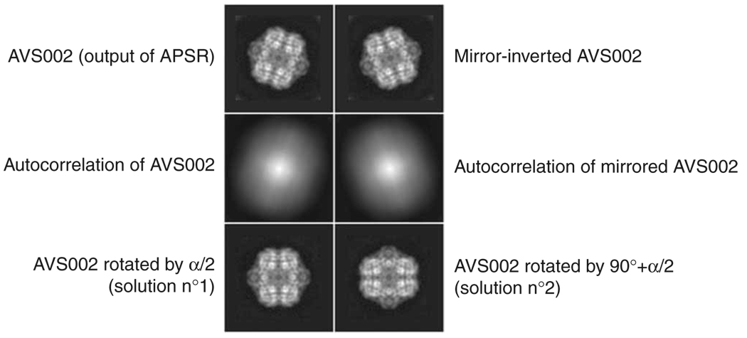
• 19Reorientation of averages. Run the batch file b04.fed. The windowed image to be used in the AP SR (http://www. wadsworth.org/spider_doc/spider/docs/man/apsr.html) operation as the initial reference is selected at random. Because of the random order in which the images are aligned, the alignment may stop after different numbers of cycles in each run. Also note that the output image obtained after alignment might not be in the best orientation to apply symmetries conveniently, or just in the best orientation for pleasing our sense of aesthetics (see Fig. 4, top left).

  To orient the particle according to its symmetry axis, the batch file b04.fed applies a mirror inversion of the output image and, using auto-correlation and angular cross-correlation functions, it finds the angle (α) necessary to align the output image to its mirror-inverted counterpart. Then, depending on the overall shape and orientation of our output image, two solutions can be applied to get a ‘vertical’ or ‘horizontal’ final orientation: either applying (α/2)° or applying (α/2)+90°. To allow for a visual check, both options are computed and put into a montage SPIDER image called ../r2d/MALIGN.hbl (Fig. 4).

• 20
  Application of alignment parameters to untilted images. At this stage, we can decide which of the two solutions we want to apply (here, it is solution 2), and move to the next step of the alignment. Hence, we have to edit batch file b05.fed and, if necessary, modify the values of parameters indicating the number of cycles produced in the previous steps:

  ;- - - - - - - - - - - - - - - - - - - - - - - - - - - - - - - - - - - - - - - - - - - -!; b05.fed/hbf: - after reference-free alignment and visual checking;              - apply solution No.1 or 2. to all original files;- - - - - - - - - - - - - - - - - - - - - - - - - - - - - - - - - - - - - - - - - - - - - - - - - - - - - - - - !; ——— Parameters ———X10 = 2 ; solution chosen No.1 or No.2 for final orientation

  Depending on which angle you choose, if running SPIDER from the command line, use X10 = 1 (for α/2°) or X10 = 2 (for (α/2)+90°). Then save your new version of the batch file b05.fed with a text editor and run it with SPIDER.

  If using SPIRE, click on the Edit button next to b05.fed and change the appropriate register, click Save and then click on b05.fed to execute the batch file. The 76 images resulting from this final alignment step are kept under the name ../images/cenu[00001–00076].hbl and the rotation angles and x/y translations applied to them are kept in the document file ../doc/dalu001.hbl. Using JWEB, you should see something as shown in Figure 5a.

• 21Centering of the 45° tilted-specimen images. Here, we want to center all the particles so that their center of gravity corresponds to the exact center of the image, but we want to keep the particles in their original orientation. Therefore, we use only the operation AP SA (http://www.wadsworth.org/spider_doc/spider/docs/man/apsa.html), which performs only half of the reference-free alignment (only the translational alignment—check also AP RA (http://www.wadsworth.org/spider_doc/spider/docs/man/apra.html), as there is an example of alignment commands using AP RA and AP SA). Look at the batch file b06.fed and run it. The images obtained after this centering step (Fig. 5b) are kept under the name../images/cent[00001–00076].hbl.
• 22Storage of the Euler angles. Run batch file b07.fed. The images correspond to several RCT series whose Euler angles phi, theta and psi were determined during the interactive particle picking (psi = azimuthal orientation of the tilt axis in our micrographs, theta = tilt angle) and during the rotational alignment on the untilted-specimen images (phi). The batch file b07.fed reads these angles and stores them in a document file ../doc/dang005.hbl.
• 23Classification of the untilted-specimen images using multivariate statistical analysis (MSA): custom-made mask (optional). We must now sort our untilted-specimen images to produce homogeneous image classes. In our case, with a small number of particles, this could be done visually, but in practice, one must rely on an automatic statistical procedure, as several thousands of images with a low signal-to-noise ratio must be sorted.

  For the analysis, we want to use only the portion of each image that corresponds to the particle. In this protocol, we could just apply a circular mask, using operation MO (http://www.wadsworth.org/spider_doc/spider/docs/man/mo.html), but as you might work on a wide variety of shapes, we show below a way to create custom-made masks that will follow the outer boundaries of your particle.

  Compute a mask that will roughly follow the outer shape of your particle. First compute the total average map of your aligned particles. The batch file b06.fed created the map ../r2d/avgu001.hbl. From this map, we will create a binary image, using the operation TH M (http://www.wadsworth.org/spider_doc/spider/docs/man/thm.html), and then operation FQ NP (http://www.wadsworth.org/spider_doc/spider/docs/man/fqnp.html) to smooth out and filter this binary image. Finally, TH M (http://www.wadsworth.org/spider_doc/spider/docs/man/thm.html) is used once more to create a new binary image from its smoothed-out version (e.g., look below and try to reproduce this mask interactively to create your own mask within subdirectory r2d/; watch out when using the TH M operation, as the threshold density will greatly change the size and shape of the output binary file).

  cd ../r2dspider hbl.OPERATION: TH M.IMAGE TO BE THRESHOLDED FILE: ../r2d/avgu001.OUTPUT FILE: scr001.BLANK OUT (A)BOVE OR (B)ELOW THRESHOLD? (A/B): B.THRESHOLD: 0.8__________________> see Box 5.OPERATION: FQ NP.INPUT FILE: scr001.OUTPUT FILE: scr0021 - LOW-PASS,       2 - HIGH-PASS3 - GAUSS LOW-PASS, 4 - GAUSS HIGH-PASS5 - FERMI LOW-PASS, 6 - FERMI HIGH-PASS7 - BUTER LOW-PASS, 8 - BUTER HIGH-PASS.FILTER TYPE (1–8): 3.FILTER RADIUS: 0.08.OPERATION: TH M.IMAGE TO BE THRESHOLDED FILE: scr002.OUTPUT FILE: ../r2d/mask01.BLANK OUT (A)BOVE OR (B)ELOW THRESHOLD? (A/B): B.THRESHOLD: 0.1______________________> see Box 5

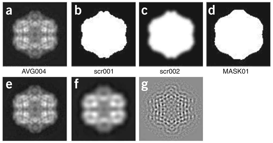
  Depending on which threshold values you use and how strongly you smooth out the first binary file, you can expand or shrink the mask (Fig. 6, panels a–d). Two operations were also developed to perform the same effects, which you can also try. They are called DI (http://www.wadsworth.org/spider_doc/spider/docs/man/di.html) to dilate and ER (http://www.wadsworth.org/spider_doc/spider/docs/man/er.html) to erode any binary map. However, they tend to form ‘squarish’ shapes, if used repeatedly. See Box 5 for information on how to apply a filter of a desired spatial frequency.

• 24
  Correspondance analysis. This version of MSA^1,32 is performed by a single operation CA S (http://www.wadsworth.org/spider_doc/spider/docs/man/cas.html). It will ask you for a prefix name (e.g., coran1), and it creates four output files corresponding to: the sequential file (SEQ), the image coordinates file (IMC), the pixel coordinate file (PIX) and the eigenvalues file (EIG). The output file names will then be formed by a concatenation of the prefix and suffix, as shown below:

  • coran1_SEQ.hbl
  • coran1_IMC.hbl
  • coran1_PIX.hbl
  • coran1_EIG.hbl

  Here, one could imagine that within a multidimensional space (e.g., here with 5,785 dimensions), each image can be represented by a single point whose coordinates are the densities contained in each of its pixels. Thus, all images taken together form a multidimensional ’cloud’. Intuitively, we can see that images that are very similar will lie close to one another, while dissimilar ones will lie far apart in this space.

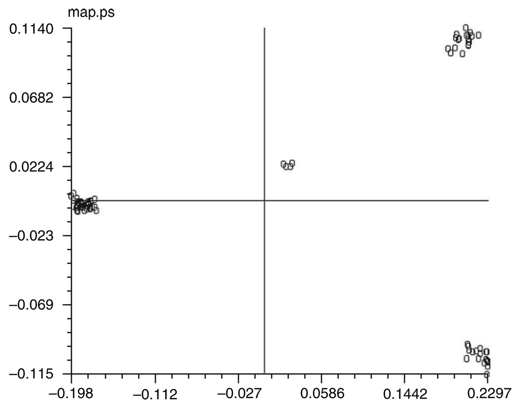
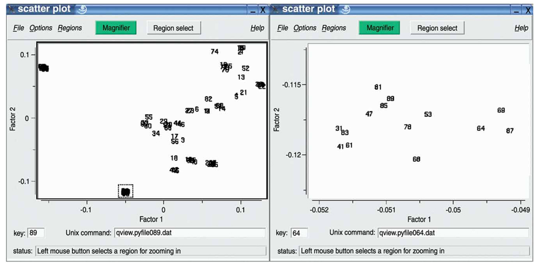
  Correspondence analysis starts by defining distances between images that are based on the χ², rather than the Euclidean metric. It proceeds by defining a new coordinate system whose axes, called ’eigenvectors’ or ’factors’, run into the directions defined by (mutually orthogonal) inter-image variance components, which can be visualized as primary extensions (length, width, etc.) of the whole cloud. In the new coordinate system, each of the images is defined by a set of new coordinates. Factors are ranked in descending order by decreasing importance, and so a much more compact representation of the image set is achieved. We can project the 76 images onto 2D planes (’factor maps’) defined by two of the seven factorial axes calculated. A projection onto the 1 versus 2 factor map (Fig. 7) immediately shows the expected grouping into 4 clusters.

  Run batch file b08.fed. In this batch file, the projection map is created as a PostScript file called ../r2d/map.ps. If you open it, you should see a map similar as the one in Figure 7.

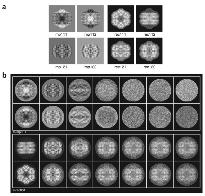
• 25Generation of importance and reconstituted images. To understand which trends correspond to factorial axes 1 and 2, we can use operations CA SRD (http://www.wadsworth.org/spider_doc/spider/docs/man/casrd.html) and CA SRA (http://www.wadsworth.org/spider_doc/spider/docs/man/casra.html) to create ‘importance’ and ‘reconstituted’ images for factorial axes 1 and 2 (Fig. 8a).

  The importance images show which pixels vary as we move along negative and positive portions of axis 1 (imp111 and imp112) and of axis 2 (imp121 and imp122). The reconstituted images show how an image would look that lies at the negative and positive extremes of each factor. Here, one can see that the negative part of axis 1 (rec111.hbl) corresponds to the hexagonal top view, whereas the positive part of axis 1 (rec112.hbl) corresponds to rectangular side views. The meaning of axis 2 is more difficult to ascertain (rec121.hbl and rec122.hbl), but it clearly expresses the variation between the rectangular side views related to the 30° rotation of the molecules.

  Run batch file b09.fed, which explores similarly the meaning of all seven factorial axes. Look at the resulting montages ../r2d/MIMP001.hbl and ../r2d/MREC001.hbl (Fig. 8b).

• 26Automatic clustering of the images (Steps 26–29). At this stage, we are going to use the simplified representation of our image set, which are the coordinates of our 76 images on seven factorial axes, to characterize automatically the different image classes. For this, we will use the hierarchical ascendant classification, which progressively merges the 76 points (corresponding to our 76 images in our new seven-axis factorial space). The merging is done in the ascending direction, i.e., the two closest points (most similar images) are first merged in a single point. The mass and location of this new point correspond to the global mass and center of gravity of the two original points. The aggregation is then resumed with the nearest next points until all the points are progressively merged into a single point. The history of aggregation is kept in a file called ‘dendrogram’ (from the Greek dendros = ‘roots’). Indeed, each merging of two points is represented by a vertical step whose height is related to the total ‘distances’ and ‘masses’ of the merged points.
  Let us see on a practical level how to run hierarchical ascendant classification. Start SPIDER and type the following commands:

  > spider hbl.OPERATION: cl hc.CORAN/PCA FILE (e.g. CORAN_01_IMC ~) FILE: ../r2d/coran1_IMC.FACTOR NUMBERS: 1–7.FACTOR WEIGHT: 0. CLUSTERING CRITERION (1–5): 5<-- Ward’s merging criterionDO YOU WANT DENDROGRAM POSTSCRIPT PLOT? (Y/T/N): N.DO YOU WANT DENDROGRAM DOC FILE? (Y/N): Y.DOCUMENT FILE: ../doc/dhac001.OPERATION: en

• 27
  Explore the results file created during this interactive SPIDER session:

  > cat results.hbl.4
  147	135	141	18	18.	0.61	*
  148	143	146	36	36.	0.75	*
  149	129	145	22	22.	7.1	****
  150	147	149	40	40.	15.	*******
  151	148	150	76	76.	2.03E+02	*****************************
  NODE	INDEX	SENIOR	JUNIOR	SIZE	HEIGHT

  Here, the highest step of the dendrogram (creating two major classes) has a height of 203, the second highest step of the dendrogram (creating a third class) has a height of 15 and the third highest step (creating a fourth class) has a height of 7.1. All subsequent steps have a height of 0.75 or less. From these results, you can decide to truncate the dendrogram between its third and fourth steps (with a threshold of 3.0, for instance). This will generate four image classes.
• 28Run b10.fed, entering the desired parameters for register X27, cutoff for branch points (here, 3.0), and register X26, Maximum dendrogram branch point (here, 203).
• 29Batch file b10.fed mentioned above will create a truncated dendrogram file psdndplot.ps. View it with any PostScript viewer (Fig. 9). You can also use JWEB to view the dendrogram, by opening dhac001.hbl as a document file and clicking on the Dendrogram tab.

  In this case, the resulting truncated dendrogram PostScript file ../r2d/psdndplot.ps looks as shown in Figure 9a.

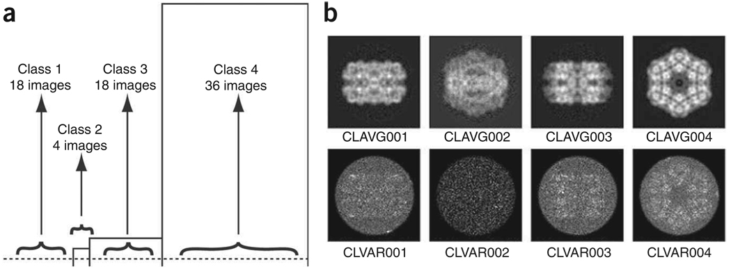
  Other outputs are document files with the lists of images corresponding to each class (../doc/dcla[001–004].hbl) and average and variance maps of each class (Fig. 9b). In this instance, we can see that classes 1 and 3 correspond to two types of rectangular side views, whereas class 4 corresponds to the hexagonal top view, and the small class 2 (only four images) corresponds to an intermediate orientation. This last, small class will not be used for the rest of the project.

  We now have three well-defined image classes from the untilted-specimen micrograph, and we know that their corresponding images windowed from the tilted-specimen micrograph produce three RCT series of projections of our particle. We also have the list of images contained in each class, and we know their Euler angles (phi, theta, psi) specifying their orientation in space. With all these information, we can compute the 3D reconstruction of our particle.

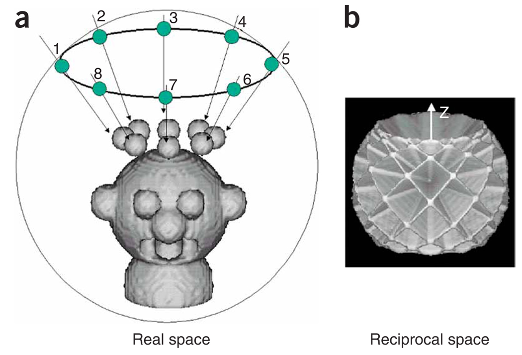
  Figure 10 shows the basic principle of the RCT-series 3D reconstruction approach. The limitation of the tilt that one can impose on the grid in the microscope induces a direct limitation of the Euler angle theta. Hence, within Fourier space (where each 2D projection corresponds to a central slice orthogonal to the projection axis), some regions remain empty. This phenomenon is responsible for the missing-cone artifact, as the empty regions correspond to two opposite cones pointing along the z axis. To prevent this missing-cone artifact, we will use the symmetries of the particle, and we will merge the different series of images to compute a global or ‘merged’ 3D reconstruction.

Figure 3.

Simulated micrograph tilt pair. (Left) Untilted-specimen micrograph. (Right) Tilted-specimen micrograph.

Figure 4.

Reference-free alignment. Reorientation of the average from reference-free alignment along the coordinate axes. The first row of this montage shows the output file and its mirror-inverted copy. The second raw of the montage shows their respective autocorrelation functions. The last two images correspond to the two solutions of our alignment (α/2)° and (α/2) + 90°.

Figure 5.

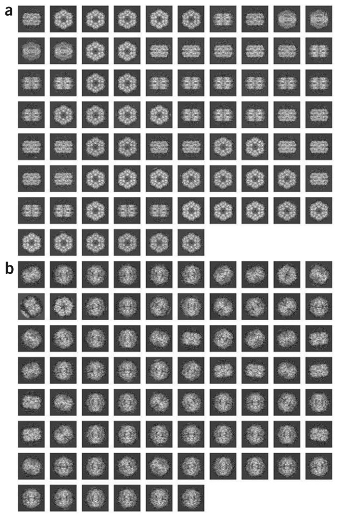
Windowed particles. (a) Montage of aligned, untilted particle images. (b) Montage of centered, tilted images.

Figure 6.

Creation of a binary mask and filtration. (a) Average image, from b06.fed. (b) Thresholded average. (c) Low-pass filtered. (d) Thresholded version of (c). (e) Original image, unfiltered. (f) Low-pass filtration at 1/35 Å⁻¹. (g) High-pass filtration at 1/25 Å⁻¹.

BOX 5 | TO APPLY A FILTER OF A DESIRED FREQUENCY.

For the filter radius, SPIDER uses units of spatial frequency in reciprocal pixels. To apply a filter of a desired frequency in reciprocal Ångstroms on the object scale, a straightforward way to determine the filter radius is to calculate the period in pixels, to know the pixel size and to take the reciprocal. Let us take the image ../r2d/avgu001.hbl (Fig. 6e) used to create the MSA mask. If the pixel size is 3.5 Å, a low-pass filtration of this image is at 1/35 Å⁻¹ resolution and the period of the desired cutoff is 35/3.5=10 pixels, or 1/10=0.10 reciprocal pixels (Fig. 6f). For a high-pass filtration at 1/25 Å⁻¹ resolution, the period is 25/3.5=7.143 pixels, or 1/7.143=0.14 reciprocal pixels (Fig. 6g).

.OPERATION: FQ NP.INPUT FILE: ../r2d/avgu001.OUTPUT FILE: scr0011 - LOW-PASS,       2 - HIGH-PASS3 - GAUSS LOW-PASS, 4 - GAUSS HIGH-PASS5 - FERMI LOW-PASS, 6 - FERMI HIGH-PASS7 - BUTER LOW-PASS, 8 - BUTER HIGH-PASS.FILTER TYPE (1–8): 5.FILTER RADIUS: 0.1 ; ----Radius in px−1.TEMPERATURE (0=CUTOFF): 0.02.OPERATION: FQ NP.INPUT FILE: ../r2d/avgu001.OUTPUT FILE: scr0031 - LOW-PASS,       2 - HIGH-PASS3 - GAUSS LOW-PASS, 4 - GAUSS HIGH-PASS5 - FERMI LOW-PASS, 6 - FERMI HIGH-PASS7 - BUTER LOW-PASS, 8 - BUTER HIGH-PASS.FILTER TYPE (1–8): 6.FILTER RADIUS: 0.14 ; ----Radius in px−1.TEMPERATURE (0=CUTOFF): 0.02

Figure 7.

Factor map. Factor 1 is the abscissa. Factor 2 is the ordinate.

Figure 8.

Importance and reconstituted images. (a) Importance (left) and reconstituted (right) images. (b) Montage of importance images (top) and reconstituted images (bottom). Note that factors 4–7 contain no information related to the variability of views but rather contain spurious noise.

Figure 9.

Clustering of images. (a) Truncated dendrogram. (b) Class averages (top) and class variances (bottom).

Figure 10.

The missing-cone artifact. (a) Projection directions. (b) Illustration of the missing cone. In reciprocal space, every 2D projection of a 3D object corresponds to a central section in the 3D Fourier transform of the object. Each central section is orthogonal to the direction of the projection. A conical tilt series allows sampling of the 3D Fourier transform of the object in all directions, except in a cone along the z axis, hence the term missing-cone artifact.

3D reconstruction of the particle

• 30Creation of the symmetry document file. To take into account the symmetries of the molecule, one must create two types of document files, describing the symmetries when the molecule is oriented in its top view (sixfold symmetry axis parallel to the z axis) or in its side view (sixfold symmetry axis parallel to the y axis).

  Run batch file b11.fed, which computes these files, named ../doc/d6top.hbl and ../doc/d6side.hbl, and which correspond to the different Euler rotation angles that allow us to superimpose the volume upon itself according to a D₆ point-group symmetry.

• 31Computation of three distinct 3D reconstructions. For the 3D reconstruction itself, we will use the BP RP (http://www.wadsworth.org/spider_doc/spider/docs/man/bprp.html) operation, which uses the simultaneous iterative reconstruction technique (SIRT) algorithm.

  Run batch file b12.fed to run these operations, but it is recommended that you use the BP RP operation in interactive mode at least once to better understand its function and adjust the values of some parameters. Here, three reconstructions corresponding to classes number 1, 3 and 4 will be computed. They are termed ../r3d/vcla001.hbl, ../r3d/vcla003.hbl, and ../r3d/vcla004.hbl.

  

• 32Manual determination of respective positions of the three reconstructions. A method to understand the orientation of the reconstructions in real space is to project them on a plane to create a pseudo cryoEM image. This can be done using operation PJ 3.
  Start SPIDER, and enter the following interactively:

  .OPERATION: PJ 3.THREED FILE: ../r3d/vcla001.PROJECTION SAMPLE DIM.: 100.OUTPUT FILE: scr001.AZIMUTH ANGLE (PHI): 0.0.TILT ANGLE (THETA): 0.0

  Here, the azimuth angle corresponds to a rotation of the object around the z axis (i.e., in the plane of the specimen grid), and the tilt angle corresponds to the real tilt angle imposed on the specimen grid within the microscope. In our example, phi and theta are set to zero, which corresponds to a projection of our reconstruction along the z axis in its original orientation, as if it were resting on the electron microscope grid.
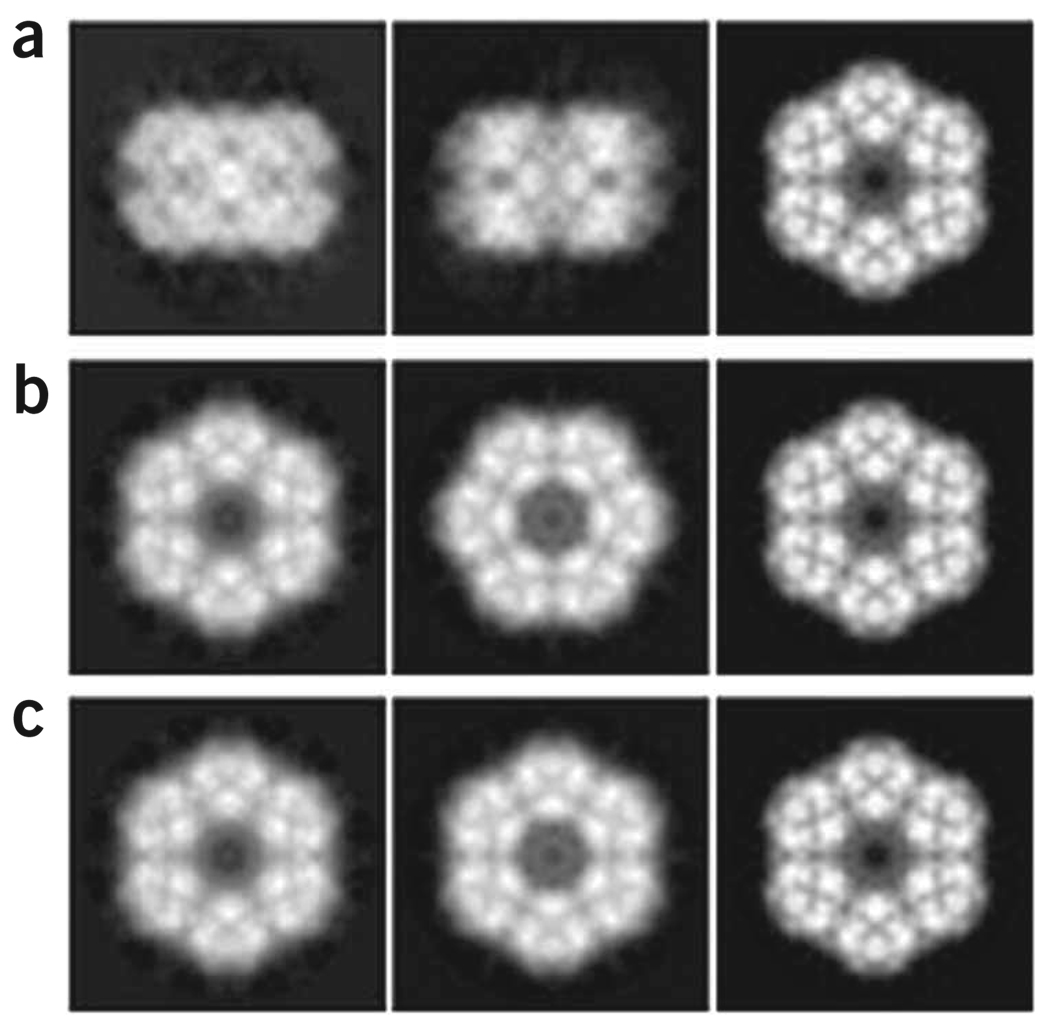
• 33Compute similar projections with the other reconstructions vcla003.hbl and vcla004.hbl, i.e., with the azimuth and tilt angles each set to zero. You will obtain images as shown in Figure 11a, comparable with the average maps of our automatic clustering on the untilted-specimen images (Fig. 9).
• 34
  To rotate a volume in space, we will use the operation RT 3D. From an interactive SPIDER session, type the following:

  .OPERATION: RT 3D.INPUT FILE: vcla001.OUTPUT FILE: VOUT001.Phi, Theta: 90.,90.Psi: -90.

  This example corresponds to a 90° rotation around the x axis.
• 35Now, similarly rotate the second reconstruction 90° around the x axis.
• 36Reproject the first two rotated reconstructions along the z axis as previously done in Step 32 (azimuth/phi and tilt/theta = 0). You will produce this new set of projections. In this panel, the first and third reconstructions are in the same orientation (Fig. 11b).
• 37To align the second reconstruction in a similar orientation, apply an additional 30° rotation around the z axis. Instead of a psi of −90, use a value of −60 (Fig. 11c).

  The batch file b13.fed computes these series of rotations shown in Steps 32 through 37, and the corresponding montages of 2D projections shown above (mpro[001–003].hbl).

• 38
  Automatic determination of relative positions of the three reconstructions. In the general case of RCT, unlike here, the exact orientations are not known in advance. SPIDER will find the best matching orientation for a pair of volumes by performing a search. This search is done stochastically from an original orientation, and the result found is not always the optimal orientation but may correspond to a local minimum searched by random jumps. Therefore, you should run this orientation search several times using different starting positions. The correlation coefficient printed at the end of the search provides an evaluation of the quality of fit (e.g., if the correlation is around 0.3, it is a poor fit, but if it is larger than 0.85, it is good). From an interactive SPIDER session, type:

  .OPERATION: OR 3QX11,X12,X13,X14.Reference 3D FILE: ../r3d/vcla004.Second FILE:../r3d/vcla001.Radius of the mask: 41..Phi, Theta: 90.,90. <----Starting position for theorientation search.Psi: -90.Iteration # 1 Distance = 0.5315237 r = 0.4684763064118FUNIQ - new parameters 90.0000 90.0000 90.0000[...]Iteration # 182 Distance = 0.1053701 r = 0.8946299150353The Euler angles found by minimization procedurePhi, theta, psi and function value90.0001 89.9993 -90.0005 0.8946275

  The batch file b14.fed starts several orientation searches and the resulting values are stored in the document file ../doc/dalv001.hbl.
• 39Merging of the three reconstructions. Rather than summing the three reconstructions after aligning them, a more elegant solution is to compute a new global reconstruction after modification of the Euler angles assigned to the images to take into account the results of the orientation search.

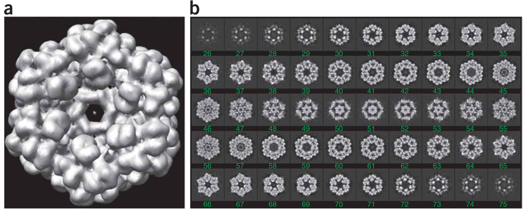
  Run batch file b15.fed. This batch file executes the following steps for each image series: (i) modifies the Euler angles; (ii) copies the images under a new name and with consecutive numbers ../images/cent[10001–10072].hbl; (iii) copies the new Euler angles with consecutive numbers in a new angular document file ../doc/dang010.hbl; and (iv) computes the global or merged reconstruction ../r3d/vtot001.hbl (Fig. 12).

Figure 11.

2D projections of 3D reconstructions for classes. (a) Projections along the z axis of reconstructions from classes 1, 3 and 4. (b) Projections after 90° rotation about the x axis for class reconstructions 1 and 3. (c) Projections after an additional rotation of 30° about the z axis for reconstruction 3.

Figure 12.

Merged reconstruction. (a) Surface rendering, using UCSF Chimera, of the 3D reconstruction vtot001.hbl, generated below by batch file b15.fed. (b) Slice series through the merged reconstruction vtot001.hbl.

Multiple common lines

• 40
  Getting started: prepare working directory. Download and unpackage commonlines.tar by typing:

  tar -xvf commonlines.tarcd Commonlines

  These steps will create a directory called Commonlines/, which contains the following:

  • common-lines batch files, ending in .cor
  • eigenhist.py: python script to generate eigenvalue histogram
  • montagefromdoc.py, .montagefromdoc: python script to view montage of particles and corresponding settings file
  • params.dat: microscopy parameters used in several steps
  • vol1class.dat (Fig. 13), vol2class.dat: reconstructions from which to generate phantom projections
  • mask_r64.dat: circular mask with radius 64 pixels, used in several steps
  • filenums.dat: list of micrographs
  • good/ngood***.dat: lists of particles for each micrograph
  • def_avg.dat: contains defocus value for each micrograph refinement batch files, in the Refinement/ subdirectory, ending in .pam
• 41To set up SPIRE (optional). If using SPIRE:

  type: spire &

  From the Project menu, select New

  Project title is required but need not be meaningful, as it is not used

  Data extension is .dat

  Set project directory to current directory (default may be Commonlines/dat)

  For Configuration file, click on the Browse button and select in the current directory commonlines.xml

  Uncheck the box Create directories and load batch files

  Click OK.

  When the form for the parameter file pops up, click Cancel. The file params.dat has already been provided.

• 42Generate random angles: weightedrandomangles.cor. This batch file will generate random orientations for each of 10,000 phantom projections. The output will contain three columns of Euler angles.

  If using SPIRE, go to Dialogs→Generate data to open the dialog containing buttons for generation of phantom data, and click on weightedrandomangles.cor.

  If not using SPIRE, go to the Commonlines/ subdirectory and then type the command:

  spider cor/dat @weightedrandomangles

  The output file prj-angles.dat will show the three Euler angles for the 10,000 projections that will be generated:

  ;cor/dat 19-JUL-2007 AT 13:28:32 prj-angles.dat
  1	3	302.58	74.453	37.168
  2	3	226.34	105.00	320.92
  3	3	8.4598	128.57	150.34
  [...]
  9998	3	326.38	86.640	350.97
  9999	3	248.70	67.703	136.14
  10000	3	146.53	60.018	140.02

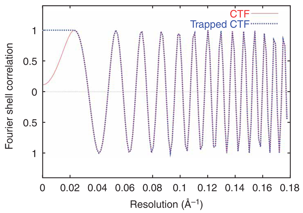
• 43
  Generate CTF filters: trapctf.cor (Steps 43–44). Run batch file trapctf.cor. This batch file generates the filters with which the images will be CTF corrected. The input file def_avg.dat looks similar to the following example:

  ;spi/dat 28-NOV-2006 AT 15:45:17 def_avg.dat
  ; /		MICROGRAPH	DEFOCUS	DEF.GROUP	DEF.GROUP.AVG
  1	4	1.00	21580.	1.00	21580.
  2	4	2.00	24833.	2.00	24833.
  3	4	3.00	26450.	3.00	26450.
  [...]
  12	4	12.0	30993.	5.00	30993.
  13	4	13.0	33150.	6.00	33150.
  14	4	14.0	34588.	7.00	34588.

  The first and second data columns list the micrograph number and defocus value, respectively. The third and fourth columns are not used. (To see how defocus value is estimated, see below in the section on projection matching.) Here, we will write out a CTF profile for each micrograph (Fig. 14).

• 44The CTF profile produced by SPIDER command TF L (http://www.wadsworth.org/spider_doc/spider/docs/man/tfl.html; red curve in Fig. 14) will dampen the lowest spatial frequencies, thus acting as a high-pass filter. To preserve the low spatial frequencies, this batch file also sets a ‘trap’ near the origin (blue curve in Fig. 14).

  Plot this profile by typing:

  gnuplot plot.gnu

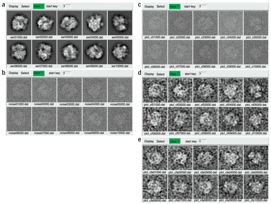
• 45Generate phantom projections: phantom.cor. Run batch file phantom.cor. This batch file applies the random orientation angles from weightedrandomangles.cor and applies the CTF profile from trapctf.cor to generate noise-free images from 14 hypothetical micrographs (Fig. 15a).
• 46
  Get image statistics: getstats.cor. Run batch file getstats.cor. This batch file records the standard deviation (s.d.) of each projection and sorts them from lowest s.d. to highest. The purpose for this step is that to set the signal-to-noise ratio—defined as the ratio of the variance of the signal to the variance of the noise—we need to know the image statistics for the different views.

  ;cor/dat 19-JUL-2007 AT 15:29:04 docsd.dat
  1	2	9967.0	1.35477E-02
  2	2	4783.0	1.35520E-02
  [...]
  4999	2	6447.0	1.57613E-02
  5000	2	6831.0	1.57616E-02
  5001	2	7921.0	1.57617E-02
  [...]
  9999	2	1904.0	1.73090E-02
  10000	2	8459.0	1.73258E-02

  Note that the first two columns of the document file are reversed for indexing. The first data column is the particle number, and the second is the s.d. Here, we will find the median value to be entered below (next section).

• 47Add noise to projections: addnoise.cor. Run batch file addnoise.cor. This batch file adds Gaussian-distributed noise to the projections. If using SPIRE, change the ‘standard deviation’ field to the median s.d. recorded from the output of getstats.cor. If not using SPIRE, use a text editor to change register [img-sd] to the median s.d.

  The default noise-to-signal ratio is set high (thus corresponding to a low signal-to-noise ratio) intentionally (Fig. 15b). In a subsequent step, we will low-pass-filter the images, which will cut out much of the noise and less of the signal on account of the different band limits of the two components.

• 48CTF-correct particles: ctfcorr.cor. If using SPIRE, go to Dialogs→Common lines to open the dialog containing buttons for common-lines alignment.

  Run batch file ctfcorr.cor. This batch file will correct for the CTF by phase-flipping (Fig. 15c).

  Note that these CTF-corrected images may look identical by eye to the initial noise-added images above (Fig. 15b). This is because (i) the amplitudes are unaffected by phase-flipping, (ii) the first zone of the CTF is not flipped and (iii) phase changes at higher spatial frequency are not readily noticeable by eye.

• 49Low-pass-filter particles: filter.cor. Run batch file filter.cor. This batch file applies a low-pass, Butterworth filter to the images (Fig. 15d). The spatial-frequency units of the pass band and stop band are given in reciprocal pixels. To convert these values to Ångstroms, divide the pixel size by the spatial frequency, i.e., in our case, 2.82/0.12 Å⁻¹ = 23.5 Å.
• 50
  Run reference-free alignment: apsr4class.cor. Run batch file apsr4class.cor, which performs reference-free alignment³¹. The number of iterations of reference-free alignment varies; in our test case, this number was eight. The alignment file 01temp008.dat looks like the following:

  ;cor/dat 19-JUL-2007 AT 16:05:55 aligndocs/01temp008.dat
  1	3	121.03	−2.6191	0.92768
  2	3	181.82	0.98035	0.59477
  3	3	213.48	1.8545	0.57318
  [...]
  9998	3	92.928	0.65883	1.1758
  9999	3	8.0175	2.0090	−0.28578
  10000	3	110.14	0.87879	4.58981E-03

  The first data column represents in-plane rotation, and the second and third columns, x and y shift, which are applied to the images (Fig. 15e).

• 51Classify particles: classify_km.cor. Run batch file classify_km.cor. This batch file runs MSA and K-means classification on the particle set.

  The entry ‘number of groups’ (register x75 if not using SPIRE) is to allow for the option to classify the particle set in groups (i.e., subsets). Here, however, we will classify all 10,000 as one set. If more than one group were used, the entry output group directory (if not using SPIRE, the label [group_dir]) can be set, e.g., to grp{**x77}.

  The entry ‘number of K-means classes’ (if not using SPIRE, register x82) is set by default to 100. With 10,000 particles, there will be on average 100 images per class. If this ratio is too low, the class averages may become too noisy, but, on the other hand, if this ratio is too high, dissimilar particles will tend to fall into the same class, which has the undesired effect of blurring the definition of the class average.

• 52Generate class averages: classavg.cor. Run batch file classavg.cor. This batch file generates class averages from the results of the classification above.
• 53
  Calculate 2D resolution: rescalc.cor. Run batch file rescalc.cor. This batch file calculates the nominal resolution from Fourier ring correlation (FRC) for each class from above.

  ;cor/dat 19-JUL-2007 AT 17:42:48 ./coran/frcdoc_final.dat
  ; /		CLASS	0.5FRC	3-SIGMA
  1	3	1.00	56.761	45.754
  2	3	2.00	33.386	29.393
  3	3	3.00	35.964	31.181
  [...]
  98	3	98.0	32.534	29.487
  99	3	99.0	39.761	28.153
  100	3	100.00	39.210	38.349

  The nominal resolution can be used as a coarse measure of the quality of a class. Low resolution (high numeric values in Ångstroms) means that the particles going into the class average are relatively dissimilar, and that the angle of the class average will not be defined very accurately in the common-lines procedure.

• 54Selection of averages (Steps 54–59). Selection of class averages will be illustrated using JWEB. To fit all 100 of the class averages in JWEB on the screen at one time, under Options→Settings, reduce the image size by a factor of, say, two.
• 55Next, go to Open→Image Series and select in the coran/ directory, avgcluster001 through avgcluster100.dat. To select a series of images, click on the first file name, and while holding down the SHIFT key, click on the last file name.
• 56When the Image Series Viewer opens, click on the Pick Particle/Categorize tab (Supplementary Fig. 4 online), and change the output Doc. File Name to coran/cat_avg.dat and click on the radio button Pick Individual Particles. (The default selection method, Pick A Set of Particles, has the user click on the first and last of contiguous series.)
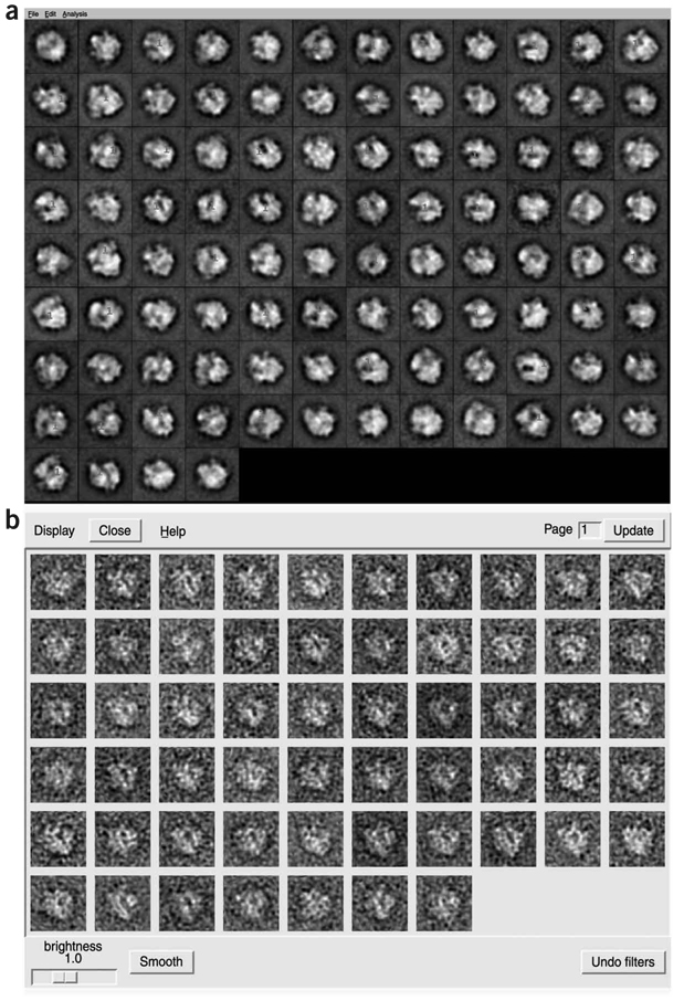
• 57Click on START, and a montage of the class averages will appear (Fig. 16a).
• 58Select the ‘good’ classes. A sharp particle boundary, a flat background, and a high resolution (from rescalc.cor above) are among the characteristics of a good class. Typically, selection of 20 or more classes is recommended for this procedure. The selected class averages are the ones that will be used in the common-lines alignment.
• 59You can see the constituent particles that make up a class by, here, using the Python script montagefromdoc.py. (There are other, equivalent ways to view the particle montage.)

  To open a montage of particles corresponding to avgcluster039.dat, type from a console window while in the Commonlines/directory:

  ./montagefromdoc.py coran/doccluster039.dat

  A pop-up window with default parameters should appear. Click Done, and a particle montage should appear (Fig. 16b). Classes of particles with low diversity in appearance (‘homogeneous classes’) are preferred.

• 60Run common-lines alignment: comlines.cor. Run batch file comlines.cor. This batch file runs common-lines alignment. Among the notable input parameters are the following:

  Number of sets of starting angles—the SPIDER command OP requires as input starting orientation angles. Here, these angles are chosen at random. To improve the chances that the correct solution will be obtained, the alignment is run several times, using several sets of starting angles.

  Number of resolution steps—the OP command asks as an input parameter the range of spatial frequencies to use for alignment of Fourier data. A priori, it is difficult to know what range to use, so the range of maximum resolutions used (the next two input registers) is searched incrementally.

  Diameter of 1D projection—Fourier transforms of 1D projections of a specified diameter will be used in the search for common lines. The length of this projection in pixels must be an odd, Fourier-friendly number. (See the note in SPIDER’s FT documentation (http://www.wadsworth.org/spider_doc/spider/docs/man/ft.html) to see forbidden values up to 1023.)

  Accuracy of theta—this parameter determines the number of reprojections used in comparison to the input class averages. Orientation assignments using a finer angle will take more time.

  Reduction factor—to speed up alignment, input images can be down-sampled. Output reconstructions will be full-sized, however.

  Maximum number of cycles—SPIDER will iteratively attempt to orient the input images, minimizing an error metric. Some orientation assignments will converge quickly, whereas others will not. In general, correct solutions will converge more quickly than incorrect ones. This criterion is not foolproof; sometimes, two more or less equally good solutions may alternate indefinitely. Among the notable output files are the following:

  Reconstructions—there will be one reconstruction for each combination of initial angles and resolution step.

  Comparison stack—this stack of images will contain a comparison of each input image used in the common-lines alignment with reprojections of the resulting reconstruction.

  Composite cross-correlation coefficient (CCC) stats—this document file is a report of each common-lines attempt, for each combination of starting angles and spatial frequency step. For example:

  ;cor/dat 23-JUL-2007 AT 20:04:18 ./commonlines/report_opg.dat
  ; /		ANGLE_SET	STEP	ANGSTROMS	PX^-1	CYCLES	AVG_CCC	AVG-MEDIAN
  1	7	1.00	1.0	47.0	0.1200	5.0	0.73291	5.33837E-03
  2	7	1.00	2.0	37.600	0.1500	200.0	0.73257	4.89831E-03
  3	7	1.00	3.0	31.333	0.1800	12.00	0.73974	1.95136E-02
  4	7	1.00	4.0	26.857	0.2100	18.00	0.73869	7.89970E-03
  5	7	1.00	5.0	23.500	0.2400	18.00	0.73869	7.89970E-03
  [...]
  41	7	9.00	1.0	47.0	0.1200	9.0	0.82867	4.13275E-03
  42	7	9.00	2.0	37.600	0.1500	200.0	0.80989	7.80898E-03
  43	7	9.00	3.0	31.333	0.1800	14.00	0.76985	1.16689E-02
  44	7	9.00	4.0	26.857	0.2100	200.0	0.81036	4.15534E-03
  45	7	9.00	5.0	23.500	0.2400	21.00	0.79224	1.83865E-02

  The first data column corresponds to the filename containing the starting angles. The second data column shows the spatial frequency step. The third data column shows the real-space resolution (expressed in Ångstroms) corresponding to the maximum spatial frequency, and the fourth column, in pixel⁻¹. The fifth column shows the number of cycles of common lines to reach convergence (or the maximum number of cycles). The sixth column is the average CCC between the input images and reprojections of the resulting reconstruction. Note that a high CCC is an indication of self-consistency and not necessarily of correctness. The seventh column shows the difference between the average CCC and the median CCC, which may be a useful metric for evaluation.

• 61Align reconstructions: volalign.cor. Run batch file volalign.cor. This batch file will align each of the reconstructions from above common-lines procedure to a reference reconstruction for the purpose of subsequent classification. If a reconstruction that is known to be correct exists, that reconstruction can be used as a reference. If not, an arbitrary reconstruction from those generated above can be used as a reference.
  Here, a reasonable choice for reference is the reconstruction with the highest average CCC with its class averages, as shown in report_opg.dat. In this instance, this reconstruction happened to be a correct one. Note, however, that this will not always be the case, so it is recommended to try different references. From the output ccvol.dat:

  ;cor/dat 24-JUL-2007 AT 11:41:07 ./commonlines/volumes/ccvol.dat
  1	7	13.0	2.00	2.00	0.36870	−57.804	−21.849	68.018
  2	7	74.0	8.00	−2.00	0.37157	37.190	24.562	−6.2177
  3	7	52.0	6.00	−1.00	0.38501	50.864	−20.249	−21.592
  [...]
  88	7	68.0	7.00	−4.00	0.98515	−22.161	44.678	−106.02
  89	7	85.0	9.00	3.00	0.98638	−65.031	12.702	28.495
  90	7	81.0	9.00	1.00	1.00	0.54120	−5.61557E-09	−0.54120
  ; /		FILENUMBER	SET	STEP	CCC	PHI	THETA	PSI

  The first column is the file number, numbered consecutively for each combination of initial orientation angles, spatial-frequency range and mirroring. The number of reconstructions compared here will be double the number of the common-lines attempts listed above in report_opg.dat. The reason for the doubling is that common-lines alignment does not distinguish between enantiomers²¹. So, each reconstruction and its mirrored analog must be aligned separately. The set of initial starting angles and resolution step are listed in the second and third data columns, respectively. A negative sign in the third data column denotes mirroring. The fourth data column is the CCC between the reference and the given reconstruction. This document file is sorted by value of CCC. If the reference was one of the reconstructions aligned, the highest CCC will be 1. A CCC greater than 0.7 generally means that the reconstruction is similar to the reference, whereas a value less than 0.5 denotes dissimilarity. The last three columns are the Euler angles relating the reconstruction to the reference.

  As an example of anticipated results, Figure 17 shows an example of slices of an aligned reconstruction that closely resemble the reference.

• 62Perform MSA on reconstructions: volmsa.cor. Run batch file volmsa.cor. This batch file runs the aligned reconstructions through MSA. Ideally, the correct solutions will cluster in factor space (Fig. 18).

  The cluster enclosed by the rectangle contains, in this case, 10 of the 16 correct solutions, and four incorrect solutions. It is important to note that there are other clusters in this factor map that do not contain correct solutions. It may be helpful to align the reconstructions to different references and run MSA on each set of aligned reconstructions.

• 63Assemble files required for refinement: copyin.cor. If using SPIRE, go to Dialogs→Refinement to open the dialog pertaining to refinement. If not using SPIRE, change to the Refinement/ subdirectory.

  Run batch file copyin.cor. This batch file prepares files required for refinement. The input parameter reconstruction number corresponds to the reconstruction number generated from volalign.cor, listed in ccvol.dat.

• 64Refine alignments: refine.pam or pub_refine.pam. The refinement batch files used here are modifications of those used later in the projection-matching section. Use the parallelized form pub_refine.pam only if you have PubSub implemented on your computer cluster. Otherwise, use the serial refinement refine.pam.

  The potential utility for refinement is to test whether correct common-lines solutions refine better than incorrect solution. In this case, the correct solution showed only a slightly better nominal resolution: 1/28.5 versus 1/30.2 Å⁻¹ (Fig. 19).

  One consideration with common lines is that there is no guaranteed internal test for correctness: CCC between class averages and reprojections, clustering of reconstructions, nominal resolution after refinement and so on. Ultimately, outside information—such as the structure of a similar complex, random-conical reconstruction and so on—is needed to verify the results from a reconstruction generated from common-lines alignment.

Figure 13.

z slices through one of the two reconstructions used to generate phantom data.

Figure 14.

CTF profiles as a function of spatial frequency. The output of SPIDER command TF L is in red. The blue curve, which preserves low spatial frequencies, will be used. Note that beyond 0.02 Å⁻¹ the two profiles are the same, appearing as a purple line.

Figure 15.

Processing of phantom data. (a) Noise-free projections of the input reconstructions. (b) Projections to which Gaussian-distributed noise has been added. (c) CTF-corrected projections. (d) Low-pass-filtered versions of projections in (c). (e) Images after reference-free alignment.

Figure 16.

K-means classification. (a) Montage of class averages. Images with a green ‘1’ were selected for common-lines alignment. (b) Montage of filtered images assigned to the same class.

Figure 17.

z slices through a common-lines reconstruction that closely resembles the correct solution.

Figure 18.

Scatter plot of factor 1 versus factor 2, generated with scatter.py. (left) and overview plot (right). Close-up view of boxed area in left. A PostScript version of factor 1 versus factor 2 is also generated by volmsa.cor.

Figure 19.

FSC curves after two iterations of refinement.

Single-particle reconstruction using the reference-based projection alignment method

• 65Initialize a Project: create a project directory with the required subdirectories and procedure files. Download reference_based.tar.gz to your working directory and unpack it by typing:

  gunzip Reference_based.tar.gz

  tar xvf Reference_based.tar

  It will create a directory called Reference_based/, containing the procedure files and subdirectories for a reconstruction project.

• 66If using SPIRE:

  go to the directory Reference_based/ and type:

  spire &

  From the Project menu, select New. Project title is required but need not be meaningful since it’s not used Data extension is .dat.

  Set project directory to current directory. (Default may be Reference_based/dat).

  For Configuration file, click on the Browse button and select in the current directory SingleParticle.xml.

  • Uncheck the box Create directories and load batch files.

  • Click OK.

  When the form for the parameter file pops up, click Cancel. The file params.dat will be generated in the next step.

• 67
  Create parameter document file. The file params.dat stores important image processing parameters used for many procedure files later. For details, see the example in the top-level directory. Run the batch file makeparams.spi interactively by typing:

  spider spi/dat @makeparams

  Follow the command-line questions as:

  .?Do the micrographs need to be unzipped(1 = yes, 0 = no)?: 0.?File format (0 = SPIDER, 1 = tif, 2 = PerkinElmer, 3 = ZI)?: 0.?pixel size (in Angstroms)?:2.82.?Electron energy (keV)?: 200.?window size (pixels)?: 130.?actual size (pixels)?: 88.?Magnification?: 50000.?scanning resolution (7,14,etc)?: 14.?decimation factor?: 1

• 68
  Create a document file filenums in the top-level project directory, containing the numbers of the files to be processed in DO loops. Run the batch file makefilelist.spi interactively by typing:

  spider spi/dat @makefilelist

  Follow the command-line questions as:

  .?Start file number: ?: 1.?Last file number: ?: 4.?output filename?: filenums

  The output file filenums.dat looks like the following:

  1	1	1.00
  2	1	2.00
  3	1	3.00
  4	1	4.00

  If you need to exclude any file from this list, use a text editor to delete the appropriate lines, then use the SPIDER operation DOC REN to renumber the lines in the document file consecutively (http://www.wadsworth.org/spider_doc/spider/docs/man/docren.html).

  Please note that due to the data set arrangement, procedures in Steps 68, 70–72, 81 and 83–88 will run only as examples. Users should need to execute these batch files, but their output files will not be used in the downstream procedures. Instead, in the respective directories, we have provided the ready-to-use output files of these procedures to be used in the downstream procedures.

• 69Prepare a 3D reference. If using your own 3D reference, copy it into the top-level project directory. If using the supplied data, it is already present as reference_volume.dat.

Single-particle reconstruction using the reference-based projection alignment method: CTF estimation

• 70Calculation of the power spectrum for each micrograph. Run batch file power.spi, which calls for subprocedure: power-p1.spi. Power spectrum of each micrograph is determined through an average of many smaller power spectra covering the area of the micrograph.

  Outputs comprise both 2D power spectra (power/pw_avg*** (Fig. 20a)) and 1D profiles of the rotationally averaged 2D power spectra (power/roo***). Procedures in this section (Steps 70–80) should be run in the Power_Spectra/ directory. The micrographs should be in the Micrographs/ directory.

• 71Evaluation of power spectrum images using JWEB. Open and examine the power spectrum image series using JWEB. (See Step 54 above for instructions on opening image series.)

  Things to look out for (Fig. 20b) are (i) are the Thon rings circular? (ii) do they extend to high resolution? Discard micrographs that show one of the following artifacts: rings that are cut off unidirectionally (evidence of drift), rings that are elliptical, or even hyperbolic (evidence of astigmatism).

• 72Estimation of defocus, astigmatism and cutoff frequency (Steps 72–77). Run batch file defocus.spi. It estimates the defocus, astigmatism and cutoff frequency at high spatial frequencies using operation TF ED (http://www.wadsworth.org/spider_doc/spider/docs/man/tfed/html).
• 73Manually verify CTF models using ctfmatch.py (http://www.wadsworth.org/spider_doc/spider/docs/spire/guitools/ctfmatch/ctfmatch.html) (Fig. 21). If not using SPIRE, type at the command line:

  ctfmatch.py &

• 74In the Set parameters window, the default parameters should be correct (2.82 Å pixels, 200 keV electrons, 2 mm spherical aberration, 0.1 amplitude contrast ratio), so click OK.
• 75Go to File→Open File series (for a single micrograph, go to File→Open TF ED file), and select the files power/ctf***. A pop-up window with a list of file names corresponding to each micrograph will appear.
• 76Click on the Defocus button (or in the main window, go to File→Open Defocus file) and select defocus_sample.dat (in Power_Spectra/).
• 77
  Next to each micrograph’s file name, the estimated defocus value (in A°ngstroms) will appear. Click on a file name, and five curves will appear:

  • in orange, the 1D profile of the power spectrum
  • in green, the background of the 1D profile
  • in red, the background-subtracted 1D profile
  • in violet, the envelope function
  • in white, the model power-spectrum profile

  For each micrograph, check whether the minima and maxima of red (or orange) and white profiles lie at the same spatial frequencies. It is helpful to multiply the (white) model power-spectrum curve by the envelope function by going to Options and clicking on the Use empirical envelope checkbutton. You can zoom in on the graph by using the y max and x min slidebars. You can adjust the defocus value, if necessary, with the defocus slidebar.

  If using X-Window WEB, manually fit CTF models to the 1D profiles of the rotationally averaged power spectra using CTF from doc file (http://www.wadsworth.org/spider_doc/web/docs/ctf.html).

• 78Group micrographs into defocus groups (Steps 78 and 79). Run batch file defsort.spi to group tentatively the micrographs that have similar defocus and assign the defocus groups.
• 79Check the defocus-group assignments using ctfgroup.py. If not using SPIRE, type at the command line:

  ctfgroup.py &

  Open the file def_sort.dat (in Power_Spectra/). The goal is to maximize the number of micrographs per defocus group, while minimizing the spread of defocus values within each group.

• 80Computation of average defocus value for each defocus group. Run batch file defavg.spi to compute average defocus value for each defocus group.

Figure 20.

Power spectra. (a) A gallery of 2D power spectra (power/pw_avg***) of a series of micrographs with different defoci. The patterns of concentric rings are the Thon rings, which reflect the different CTFs. (b) A gallery of 2D power spectra with examples of problems. Question marks indicate power spectra that fall off rapidly after the first plateau.

Figure 21.

Manual fitting of a CTF model to a 1D power spectrum profile (power/roo***) using ctfmatch.py.

Single-particle reconstruction using the reference-based projection alignment method: particle picking and selection

• 81Generate a background noise file (Steps 81 and 82). A background noise image is used to normalize the backgrounds of the particle images³³. Run batch file noise.spi, which generates a set of images (tmpnoise/noi***) from random regions in the micrograph that appear not to contain any particles. The batch file requires as its input a randomly picked micrograph (e.g., mic001.dat).

  Procedures in this section (Steps 81–88) should be run in the Particles/ directory.

• 82View these noise images in JWEB and select one that does not have any structure and copy it into Particles directory as noise.dat.
• 83Run automatic particle picking. Choose one of the two following approaches: option A to correlate against a Gaussian blob or option B to use a fast locally normalized correlation algorithm.

  1. Apply cross-correlation of the micrographs with a Gaussian blob (works best with globular particles such as ribosome or GroEL)

     1. Run batch file pick.spi, which calls for subprocedures: pick-p.spi, convert-p.spi.

     2. The micrographs are decimated, low-pass-filtered and searched for peaks over regions corresponding to particle dimensions. ‘Decimation’ means that every nth pixel is used (n being in the range of 4 to 6 for particle picking) and the rest discarded.

     3. Particle candidates windowed out and centered are stored as win/ser*****, and their coordinates on the corresponding micrographs are stored in documents coords/ndc*** (peak coordinates from the ×4 decimated image) and coords/sndc*** (top left pixel coordinates for particle images).

  2. Apply fast normally localized correlation algorithm

     1. This approach uses a fast locally normalized correlation algorithm outlined by Roseman³⁴. The detailed implementation as a SPIDER procedure was described by Rath and Frank³⁵.

     2. Run batch file lfc-pick.spi, which calls for subprocedures pickparticle.spi, convert-p.spi.

     3. The local normalization procedure eliminates long-range density fluctuations (‘ramps’, etc.) in the searched image and hence reduces misidentifications of noise peaks in the CCF as particles. As the computation of the local normalization is done in Fourier space, the computation is very fast.

     4. A 3D reference map is required as input to generate projections optionally at desired Eulerian angles for searching different orientations of the particle images in the micrographs.

     5. Output files include particle images (win/ser*****) and pixel coordinates for center of particle images (coords/sndc***).

• 84Determination of particle numbers corresponding to each micrograph. Run batch file pnums.spi. The output file order_picked lists the particle number associated with each micrograph.
• 85(Optional) Filter the particle images. Run batch file pfilt.spi. Manual selection of good particles (the next step) is easier if the particles have been low-pass-filtered. A low-pass Butterworth filter is applied here. The filtered particle images are stored as flt/ser***** (Fig. 22). The batch file will ask for the last particle number, which you can get from the output of pnums.spi, order_picked.dat.
• 86
  Verify the automatically selected particle images and eliminate any nonparticle image. There are three options for particle verification: option A to use JWEB, option B to use montagefromdoc.py and option C to use X-window WEB.

  1. JWEB
     1. To fit a large number of particles on the screen, under Options→Settings, reduce the image size by a factor of, say, two. Next, go to Open→Image Series and select in the win_sample/ directory a convenient number of ser***** files (or flt/ser*****). When the Image Series Viewer opens, click on the Pick Particle/Categorize tab. Change the output Doc. File Name to good/good*** (substituting the appropriate micrograph number) and click on the radio button Pick Individual Particles. When the particle images are displayed on the screen, use the mouse to click on each good particle. Refer to the file order_picked.dat to ensure that particles from only a single micrograph are displayed in an image series, i.e., that the selection does not straddle two micrographs. Note that each time you open a new image series, you will need to reset the Doc. File Name.
  2. montagefromdoc.py.
     1. montagefromdoc.py is a Python/Tkinter program to pick particles. From the Particles directory, type the following: montagefromdoc.py (or, if the current directory is not in your $PATH, type ./montagefromdoc.py). A pop-up window will appear with hopefully appropriate defaults, e.g.,
        • doc_file—coords/sndc0001.dat
        • particle_template—flt/ser******.dat
        • output_file—good/good001.dat
     2. Clicking OK will open a 17×9 montage of particles. The PageDown and PageUp keys will cycle through other screenfuls. (Other keyboard commands are shown in the menu under Help→Keyboard shortcuts.) Clicking on a particle will select it, and clicking a second time will deselect it. Save the list of picked particles using File→Save selection in the menu.
  3. X-Window WEB
     1. Use the operation Categorize from sequential montage. For each micrograph, save your selections to a document file named good/good***.
        The images selected will be those used in alignment. Also, the images used to compute the 3D reconstruction will be selected from this set.
• 87Remove any duplicated particles. Run batch file renumber.spi. When manually selecting particles in the previous step, sometimes a particle is accidentally double-clicked. This procedure will delete the appropriate lines from the file.
• 88List percentages of selected particles. Run batch file snums.spi. Outputs include order_selected, a document file listing selected particles for each micrograph, and percent_selected, listing percentages of automatically picked versus manually selected particles.

Figure 22.

Examples of particle images before (top) and after filtering (bottom).

Single-particle reconstruction using the reference-based projection alignment method: reference-based alignment

• 89
  Create a set of 2D reference projections for alignment from a 3D reference map. Run batch file refproj.spi. The following output files are generated:

  • projlist: document file listing the reference projection numbers. For instance, with angular interval set to 15°, a total of 83 projections are generated.
  • refangles: document file listing the three Euler angles for all the 83 projections, generated by operation VO EA (http://www.wadsworth.org/spider_doc/spider/docs/man/voea.html).
  • prj_***: image stack files of reference projections (Fig. 23a). Generated with the operation PJ 3Q (http://www.wadsworth.org/spider_doc/spider/docs/man/pj3q.html) using the two files mentioned above. For each defocus group, a set of reference projections is generated by applying the CTF of the defocus group that the particle projections belong to. The idea is that with matched CTF applied to the reference projections, the CCF peak value is maximized.
  • Procedures in this section (Steps 89–92) should be run in the Alignment/ directory.
• 90Prepare document files used in alignment. Run batch file sel-by-group.spi. Outputs are part_by_group_*** (listing all the particles in each defocus group) and order_defocus (listing number of particles, cumulative number of particles and average defocus for each group).
• 91Align particle images to the reference projections using operation AP SH (http://www.wadsworth.org/spider_doc/spider/docs/man/apsh.html). Run batch file apshgrp.spi. Outputs contain shift and rotation parameters for the best-matched projections (align_01_***).
• 92Rotate and shift particle images according to alignment parameters. Run batch file alignsh.spi. Outputs are aligned particle images stored as ali/sar*****.

Figure 23.

Multiple references. (a) Gallery of 83 projections of the reference. (b) Averaged particle images in a single defocus group.

Single-particle reconstruction using the reference-based projection alignment method: compute averages

• 93
  Make selection document files listing particles for each projection. Run batch file select.spi. Outputs are as follows:

  • df***/how_many: number of particles associated with each reference view for each defocus group.
  • df***/select/sel***: particles associated with each reference view for each defocus group.
  • how_many: total number of particles associated with each reference view.

  Procedures in this section (Steps 93–103) should be run in the Reconstruction/ directory.

• 94Create average images for all the projection groups (Steps 94 and 95). Run batch file average.spi. Outputs are average images for each projection group (avg/avg***) and variance images for each projection group (avg/var***).
• 95In JWEB, view the set of average images. Projection views with many particles will have averages that resemble the reference projection (Fig. 23b). Projection views with few particles will be noisy.
• 96Identify a threshold correlation coefficient for selecting true particles. Run batch file cchistogram.spi, which creates a histogram for each defocus group that plots the number of particles versus the cross-correlation value. Outputs are histograms by defocus group (hist/cchist_***) and a histogram of all groups (hist/cchist_all).
• 97Plot histograms using Gnuplot (Steps 97 and 98). Run batch file plothist.spi. The output (plot_hist.dat) is a text file containing Gnuplot commands for displaying the histogram for all particles. The histograms by defocus group can be plotted in a similar way.
• 98To display the plot (Fig. 24), from the command line, type gnuplot to start Gnuplot, then at the Gnuplot prompt, type

  load ‘plot_hist.dat’.

  If the histogram displays a bimodal distribution, the higher peak may correspond to actual particles, whereas the lower peak may show noise. A threshold should be chosen between two such peaks.

• 99Compute thresholds of cross-correlation for discarding particles. Run batch file ccthresh.spi. Given a percent cutoff level (stored in register x30), this batch file creates a document file thresh.dat, containing thresholds for each defocus group. For example, if a percent cutoff of 0.20 is used (x30 = 0.2), then 20% of all particles with lowest cross-correlation values will be rejected.

  The correlation thresholds in thresh.dat may be edited, if you wish to use different cutoff levels.

• 100Select particles above the correlation thresholds. Run batch file dftotals.spi. Outputs (df***/seltotal) list the particles with cross-correlation values greater than the threshold.
• 101Check the distribution of particles among all the reference views. Run batch file plotview.spi. This procedure creates a text file of Gnuplot commands plot_view.dat, which plots the document file how_many.dat, showing the number of particles versus projection view (Fig. 25a).
• 102Generate SPIDER image files showing the number of particles per projection view (Steps 102 and 103). Run batch file display.spi, which calls for sub-procedure display-p.spi.
• 103In JWEB, display the output files (display/cndis***), which show the angular reference groups represented by small circles (Fig. 25b). The areas of these circles are proportional to the numbers of particles in each group.

Figure 24.

Correlation histogram of all particles.

Figure 25.

Distribution of orientations. (a) Histogram of number of particles versus projection view. (b) Map of angular coverage. Numbers in circles denote the Eulerian angles (ordered in a spiral outgoing from the pole); areas of circles are proportional to numbers of particle projections falling into that direction.

Single-particle reconstruction using the reference-based projection alignment method: generation of an initial reconstruction

• 104
  Split the data, create paired reconstructions and compute resolution for each defocus group. Run batch file deffsc.spi. This procedure uses the back-projection method (operation BP RP (http://www.wadsworth.org/spider_doc/spider/docs/man/bprp.html)) and creates two half-reconstructions for each defocus group by splitting the data into two equal sets (each with odd- and even-numbered particles, respectively). The reconstruction resolution of each defocus group is calculated by comparing the two half-reconstructions (operation RF 3 (http://www.wadsworth.org/spider_doc/spider/docs/man/rf3.html)). Important outputs are as follows:

  • df***/vol001_odd: reconstructed map from odd numbered images for each defocus group.
  • df***/vol001_even: reconstructed map from even numbered images for each defocus group.
  • df***/doccmp001: Fourier shell correlation (FSC) curve for map in each defocus group:

  Procedures in this section (Steps 104–108) should be run in the Reconstruction/ directory.

• 105
  Apply CTF correction, create an initial reconstruction and compute the combined resolution. Run batch file ctf.spi. This batch file applies CTF correction using Wiener filtering³⁶ to all the defocus groups (operation TF CTS (http://www.wadsworth.org/spider_doc/spider/docs/man/tfcts.html)) and creates a reconstruction from the entire data set. Finally it calculates the FSC resolution curve for the combined data set (operation RF 3 (http://www.wadsworth.org/spider_doc/spider/docs/man/rf3.html)). Outputs include the following:

  • vol001 3D structure from the entire set of particles. It is known as the ‘initial reconstruction’ and will be used as the input for the refinement step.
  • combires FSC curve for the initial reconstruction from the combined data set.
• 106Determine resolution of the initial reconstruction using 0.5 cutoff of FSC. Run batch file res.spi. This batch file computes the FSC between the odd and even reconstructions.
• 107
  Plot the resolution curve of each defocus group, along with the combined resolution curve. Run batch file plotres.spi. This batch file creates a text file of Gnuplot commands plot_res:

  set xlabel ‘‘Frequency’’set title ‘‘FSC: 0.5 resolution = 17.90 Angstroms’’plot \‘‘df001/doccmp001.dat’’ using 3:5 title ‘‘dfg001’’ with lines, \‘‘df002/doccmp001.dat’’ using 3:5 title ‘‘dfg002’’ with lines, \‘‘df003/doccmp001.dat’’ using 3:5 title ‘‘dfg003’’ with lines, \‘‘df004/doccmp001.dat’’ using 3:5 title ‘‘dfg004’’ with lines, \‘‘df005/doccmp001.dat’’ using 3:5 title ‘‘dfg005’’ with lines, \‘‘df006/doccmp001.dat’’ using 3:5 title ‘‘dfg006’’ with lines, \‘‘df007/doccmp001.dat’’ using 3:5 title ‘‘dfg007’’ with lines, \‘‘combires.dat’’ using 3:5 title ‘‘Combined’’ with lines

  A screen capture of the plot is shown in Figure 26a. The nominal resolution is where the Fourier shell correlation drops below the threshold (0.5). Identify the corresponding spatial frequency (resolution distance = pixel size/spatial frequency, here 17.90 Å).

• 108Filter the initial reconstruction Run batch file filt.spi. Low-pass-filter the initial reconstruction at the cutoff frequency (Fig. 26b). Use the Surface operation in JWEB to view the filtered reconstruction.

Figure 26.

Initial reconstruction. (a) FSC curves for all defocus groups, and for the combined set. (b) Surface rendering of the initial reconstruction (map filtered at 17.9 Å).

Single-particle reconstruction using the reference-based projection alignment method: angular refinement

• 109The angular refinement is a computationally expensive operation. Before running the refinement procedure files, check the results of the above reconstructions, to ensure that all defocus groups have reasonable-looking reconstructions. Procedures in this section (Steps 109–113) should be run in the Refinement/ directory.
• 110Create a document file summarizing the selected particles. Run batch file ordselect.spi. The output file (order_select.dat) contains number of particles and defocus value in each group.
• 111Generate the data file stacks and alignment parameter files. Run batch file stack.spi. The purpose of using stack files is to speed up the computation. Multiple images can be stored within a single SPIDER ‘stack file’. Here, the selected original particles are stored as input/data*** and selected aligned particles are stored as input/dala***.
• 112SPIDER refinement (http://www.wadsworth.org/spider_-doc/spider/docs/techs/recon/refine.html). Angular refinement is the most complex procedure and requires a set of SPIDER procedure files. To be distinguishable from other procedure sets, all the procedure files used in the refinement have the same extension pam.

  Procedures include the following:

  refine.pam—main procedure

  refine_settings.pam—stores all the parameters needed to be set

  sort.pam—sorts defocus groups by particle numbers for computing efficiency

  prepare.pam—automatically prepares required initial files

  newdala.pam—prepares stack files for aligned particles

  grploop.pam—in each iteration, for each defocus group, aligns particle images against the reference projections (operation AP REF (http://www.wadsworth.org/spider_doc/spider/docs/man/apref.html)), constructs reconstructions using fast backprojection method in Fourier space (operation BP 32F (http://www.wadsworth.org/spider_doc/spider/docs/man/bp32f.html)) and calculates FSC curves

  mergegroups.pam—at the end of each iteration, performs CTF correction using Wiener filtering (operation TF CTS (http://www.wadsworth.org/spider_doc/spider/docs/man/tfcts.html)) on reconstructions from all the defocus groups

  saveresp.pam—calculates resolution using 0.5 cutoff of FSC

  endmerge.pam—at the end of the last iteration, recalculates reconstructions for each defocus group using the accurate conjugate gradients method (operation BP CG (http://www.wadsworth.org/spider_doc/spider/docs/man/bpcg.html))

  endrefine.pam—at the end of the last iteration, generates the final reconstruction (bpr**) by applying CTF correction using Wiener filtering (operation TF CTS (http://www.wadsworth.org/spider_doc/spider/docs/man/tfcts.html)) on reconstructions from all the defocus groups and calculates the FSC curve of the final, merged reconstruction (dbpr**)

  smangloop.pam—used for refinement with small angular increment (optional)

  enhance.pam—applies Fourier amplitude enhancement (optional)

  Check the parameters and file names in refine_settings.pam and then run batch file refine.pam.

• 113
  Plot the refinement resolution curves. Run batch file plotref.spi. It creates two text files of Gnuplot commands:

  • plot_refi: plots combined resolution curve for each iteration (Fig. 27a).
  • plot_refd: plots combined resolution curve and curves from each defocus group resolution for the last iteration (Fig. 27b).

  Figure 27c shows surface presentations of the initial reconstruction (left) and the final, refined reconstruction (right).

Figure 27.

Refined reconstruction. (a) FSC curves for each iteration. (b) Refined (last iteration) FSC curve of each defocus group, along with the combined resolution curve. (c) Comparison of initial (left, 17.9 Å) and refined (right, 16.0 Å) reconstructions.

Single-particle reconstruction using the reference-based projection alignment method: amplitude correction

• 114Generate a power-spectrum profile for the EM map. Run batch file power-check.spi. This batch file generates a 1D power-spectrum profile and plots it in comparison to the X-ray scattering profile and the FSC (Fig. 28a).

  Procedures in this section (Steps 114–117) should be run in the Amplitude_Correction/ directory, or from the Amplitudes dialog box in SPIRE.

• 115Create an enhancement curve for the EM map. Run batch file enhance.spi, which calls for subprocedure pwsc.spi and Gnuplot script plotfit. The batch file enhance.spi computes an enhancement curve, by comparing a 1D rotationally averaged power spectrum of the EM map to the X-ray solution scattering amplitude (scattering_70s.dat). This curve represents the correction by which the EM map’s power spectrum must be multiplied to raise it to the X-ray curve.
• 116Generate a smooth enhancement curve by fitting a polynomial to the original one. If using SPIRE, the enhancement curve (Fig. 28b) produced by the Gnuplot script plotfit will appear automatically. An iterative fitting will be applied using polynomial ‘K(x) = A* x* x + B’, in which K(x) is the original enhancement curve and A and B are two fitting parameters. When the Gnuplot window is closed, the fitting information from Gnuplot will appear in the SPIRE main window. Note the fitting parameters A and B.
• 117Apply the fitted enhancement curve to the reconstruction. Run batch file applyabc.spi. Using the parameters obtained above (here, A = 121.868; B = 61,431.1), apply the enhancement to the EM map, and filter the enhanced map at the resolution level.

  Upon amplitude correction, local features appear sharper as an effect of the enhancement of amplitudes in the high spatial frequency range. The effect is more pronounced in a higher-resolution map (Fig. 29).

Figure 28.

Amplitude-enhancement profiles. (a) Profiles of Fourier shell correlation, Fourier amplitudes of the EM map (bpr06.dat) and the low-angle X-ray solution scattering data. (b) Fitting of the enhancement curve.

Figure 29.

Effect of amplitude enhancement. (a) Comparison of maps before (left) and after (right) the Fourier amplitude correction. (b) Effect of amplitude correction on a 9.9-Å EM map (reconstructed from the same data set described in this protocol, using original 91,114 particles).

Single-particle reconstruction using the reference-based projection alignment method: supervised classification

• 118Choose proper reference maps representing the two presumed conformers in the data set. In this example, we use maps of two ribosomal complexes related by a ratchet-like motion (Fig. 30, shown in Fig. 13 as slices), both provided in the top-level directory.

  Procedures in this section (Steps 118–130) should be run in the Classification/ directory, or from SPIRE from the Classification dialog.

• 119Creation of a set of 2D reference projections. Run batch file refproj.spi, which creates a set of 2D reference projections for alignment for the second reference map.
• 120Preparation of selection files used for reference map. Run batch file sel-by-group.spi, which prepares document files used in alignment for the second reference map.
• 121Align particle images to the second reference map. Run batch file apshgrp.spi, which aligns particle images to the second reference map.
• 122Recalculate alignments. Run batch file sc-apsh.spi, which recalculates alignments for particles that assigned to different views for the two reference maps. Only the view that yields the higher CC is chosen.
• 123Normalization of cross-correlation coefficients. Run batch file sc-norm.spi, which normalizes the CC for each reference, i.e., rescales from 0 to 1.
• 124Calculate CC2 − CC1 (Δ CC) for all the particles. Run batch file sc-compare.spi. This procedure creates two document files, align_sc_diff.dat (stores ΔCC for each particle) and hist_sc_diff.dat (stores number of particles versus ΔCC).
• 125Plot the distribution of number of particles versus Δ CC. Run batch file plotdiff.spi. This procedure creates a text file of Gnuplot commands plot_diff.dat, which plots the distribution of particle resemblance (hist_sc_diff.dat) with respect to the two references.
• 126Creates particle list for each chosen subset, according to the particle distribution above. Run batch file sc-select.spi. On the basis of Figure 31, we divided the entire data set into two subsets, along the x axis: subset no. 1, −0.01 to 0.4 (including 5,834 particles); subset no. 2, −0.4 to −0.01 (including 4,166 particles).

  Steps 126–130 should be performed on each of the two subsets chosen from the histogram in Figure 31. In SPIRE, Steps 126–129 are enclosed in a box labeled with a reminder. For Step 130 (refinement), SPIRE has a separate dialog for each of the two subsets.

• 127Separation of selection list for subset by defocus group. Run batch file sc-dfsel.spi, which separates the selection list for a subset by defocus group.
• 128Creation of reconstructions and computation of resolution for each defocus group. Run batch file deffsc.spi, which creates paired reconstructions and computes the resolution for each defocus group.
• 129CTF correction and computation of combined resolution. Run batch file ctf.spi, which applies CTF correction and computes the combined resolution.
• 130Refinement. Repeat refinement for each class (Steps 109–112). That is,

  ordselect.spi

  stack.spi

  refine.pam (serial) or pub_refine.pam (parallelized)

  plotref.pam

  Run these batch files from the Classification/Refinement1/ or Classification/Refinement2/ directories. If using SPIRE, there are separate dialogs for each class called Class 1 Refinement and Class 2 Refinement.

Figure 30.

Reference maps used for supervised classification. These maps differ in the degree of ‘ratchet’ rotation of the 30 versus 50S subunit²⁶. (a) Unratcheted ribosome. (b) Ratcheted ribosome.

Figure 31.

Distribution of particle resemblance with respect to the two references (red curve), which reveals a possible bimodel distribution. Here, the data set is divided into two subsets at ΔCC= −0.01 (green line).

Random-conical reconstruction

Step 1, getting started: depends on network speed; TAR files total about 3.6 MB

Steps 3–13, interactive particle picking, using JWEB: ~10 min

Step 18, two-dimensional alignment of the untilted-specimen images: <1 min

Step 20, application of alignment parameters to untilted images: <1 min

Step 21, centering of the 45° tilted-specimen images: <1 min

Step 22, storage of the Euler angles: <1 min

Step 23, classification of the untilted-specimen images using MSA: custom-made mask (optional): ~3 min

Step 24, correspondence analysis: <1 min

Step 25, generation of importance and reconstituted images: <1 min

Steps 26–29, automatic clustering of the images: ~3 min

3D reconstruction of the particle

Step 31, computation of three distinct 3D reconstructions: ~20 min if using BP RP and ~3 min if using BP 3F

Step 32, manual determination of respective positions of the three reconstructions: <1 min

Step 38, automatic determination of respective positions of the three reconstructions (optional): <1 min

Step 39, merging of the three reconstructions: ~20 min if using BP RP and ~4 min if using BP 3F

Multiple common-lines

Step 40, getting started: prepare working directory: depends on network speed, TAR files total about 18 MB.

Step 41, to set up SPIRE (optional): ~1 min

Step 42, generate random angles: weightedrandomangles.cor: <1 min

Step 43, generate CTF filters: trapctf.cor: <1 min

Step 45, generate phantom projections: phantom.cor: ~10 min

Step 46, get image statistics: getstats.cor: ~1 min

Step 47, add noise to projections: addnoise.cor: ~3 min

Step 48, CTF-correct particles: ctfcorr.cor: ~2 min

Step 49, low-pass-filter particles: filter.cor: ~7 min

Step 50, run reference-free alignment: apsr4class.cor: ~20 min

Step 51, classify particles: classify_km.cor: ~40 min

Step 52, generate class averages: classavg.cor: ~3 min

Step 53, calculate 2D resolution: rescalc.cor: ~2 min

Steps 54–59, selection of averages: ~10 min

Step 60, run common-lines alignment: comlines.cor: 3 h

Step 61, align reconstructions: volalign.cor: ~15 min

Step 62, perform MSA on reconstructions: volmsa.cor: 30 min

Step 63, assemble files required for refinement: copyin.cor: 2 min

Step 64, refine alignments: refine.pam or pub_refine.pam: ~8 h

Single-particle reconstruction using the reference-based projection alignment method

Step 65, initialize a Project: create a project directory with the required subdirectories and procedure files: depends on network speed, TAR files total about 800 MB

Step 67, create parameter document file: <1 min

CTF estimation

Step 70, calculation of the power spectrum for each micrograph: ~1 min

Step 71, evaluation of power spectrum images using JWEB: ~1 min

Step 72, estimation of defocus, astigmatism and cutoff frequency: <1 min

Steps 78 and 79: group micrographs into defocus groups: <1 min

Step 80, computation of average defocus value for each defocus group: <1 min

Particle picking and selection

Steps 81 and 82, generate a background noise file: <1 min

Step 83, run automatic particle picking: ~10 min

Step 84, determination of particle numbers corresponding to each micrograph: <1 min.

Step 85, filter the particle images: ~5 min

Step 86, verify the automatically selected particle images and eliminate any nonparticle image: ~1 h

Step 87, remove any duplicated particles: <1 min

Reference-based alignment

Step 89, create a set of 2D reference projections for alignment from a 3D reference map: <1 min

Step 90, prepare document files used in alignment: <1 min

Step 92, rotate and shift particle images according to alignment parameters: ~5 min

Compute averages

Step 93, make selection document files listing particles for each projection: <1 min

Step 94, create average images for all the projection groups: <1 min

Step 95, view the set of average images:<1 min

Step 96, identify a threshold correlation coefficient for selecting true particles: <1 min

Steps 97 and 98, plot histograms using Gnuplot: <1 min

Step 99, compute thresholds of cross-correlation for discarding particles: <1 min

Step 100, select particles above the correlation thresholds: <1 min

Step 101, check the distribution of particles among all the reference views: <1 min

Steps 102 and 103, generate SPIDER image files showing the number of particles per projection view: <1 min

Generation of an initial reconstruction

Step 104, split the data, create paired reconstructions and compute resolution for each defocus group: ~1 h

Step 105, apply CTF correction, construct an initial reconstruction and compute the combined resolution: <1 min

Step 106, determine resolution of the initial reconstruction using 0.5 cutoff of FSC: <1 min

Step 107, plot the resolution curve of each defocus group, along with the combined resolution curve: <1 min

Step 108, filter the initial reconstruction: <1 min

Angular refinement

Step 110, create a document file summarizing the selected particles: <1 min

Step 111, generate the data file stacks and alignment parameter files: ~5 min

Step 112, SPIDER refinement: ~6 h

Step 113, plot the refinement resolution curves: <1 min

Amplitude correction

Step 114, generate a power-spectrum profile for the EM map: <1 min

Step 115, create an enhancement curve for the EM map: <1 min

Step 116, generate a smooth enhancement curve by fitting a polynomial to the original one: <1 min

Step 117, apply the fitted enhancement curve to the reconstruction: <1 min

Supervised classification

Step 119, creation of a set of 2D reference projections: < min

Step 120, preparation of selection files used for reference map: < min

Step 121, align particle images to the second reference map: ~1 h

Step 122, recalculate alignments: ~10 min

Step 123, normalization of cross-correlation coefficients: < min

Step 124, calculate CC2 - CC1 (ΔCC) for all the particles: < min

Step 125, plot the distribution of number of particles versus ΔCC: < min

Step 126, creates particle list for each chosen subset, according to the particle distribution above: <1 min

Step 127, separation of selection list for subset by defocus group: <1 min

Step 128, creation of reconstructions and computation of resolution for each defocus group: ~30 min

Step 129, CTF correction and computation of combined resolution: <1 min

Step 130, refinement: ~5 h

Step 7

If you make a mistake and select the wrong particle, you can correct this mistake by clicking the right button of the mouse before resuming your selection.

Step 13

If you encounter some problems during particle picking with the JWEB software, you can still do the rest of the tutorial because we already put particle-picking document files (dcu001.hbl, dct001.hbl, dcb001.hbl) in the doc/ subdirectory.

Step 20

If your rectangular views are rotated 90° compared with these images, then it means that you chose the wrong final rotation angles above. In this case, you should modify the value of X10 in batch file b05.fed and run it again.

Step 31

If BP RP is too slow on your machine, or if you are in a hurry, check the end of batch file b12.fed, where the use of operation BP 3F (http://www.wadsworth.org/spider_doc/spider/docs/man/bp3f.html), which uses direct Fourier methods, is implemented but commented out. Reconstructions can be checked, using surface rendering in UCSF Chimera (http://www.cgl.ucsf.edu/chimera/), for example.

Step 39

As with batch file b12.fed mentioned above, if operation BP RP is too slow, operation BP 3F is implemented but commented out.

Step 70

If SPIDER exits with an error message, often the first place you should look in is the Results file. Look at the last few lines of the results file for useful diagnostic information.

Some common errors:

*** DOC FILE DOES NOT EXIST: ../filenums.hcc

*** FILE NOT FOUND: ../Micrographs/mic0001.hcc

Make sure that the file exists and that the path is correct.

Also check the file numbering in the batch file. The number of digits in the file name must match the number of asterisks in the variable name, e.g., for [i] = 1, mic{****[i]} matches mic0001.dat, but not mic01.dat

*** SUBSTITUTING: 123 INTO: mic{**[i]} DAMAGES INVARIANT PART OF STRING

There are not enough asterisks to represent the three-digit number. Use more asterisks.

*** ERROR OPENING FILE: power/pw_avg0001.hcc

Make sure the output directory exists.

*** ERROR: PROCEDURE FILE.spi DOES NOT EXIST

SPIDER cannot find the batch or procedure file. Make sure the SPIDER command ‘spider ext/dat @procname’ correctly specifies the desired procedure file. If the batch file calls for additional procedures, they must have the same file name extension as the calling batch file.

Step 116

If Gnuplot pop-up window does not open, first type gnuplot to start Gnuplot, then under the prompt of Gnuplot, type load ‘plotfit’.

ANTICIPATED RESULTS

Expected outcomes of this protocol are described throughout PROCEDURE. Finally, we obtained two refined maps at resolutions of 18.1 and 18.5 Å, from two subsets, separately (Fig. 32).

Figure 32.

Reconstructions from two subsets using supervised classification. The map no. 1 (left) is reconstructed from subset no. 1 using 5,834 particles and map no. 2 (right) is reconstructed from subset no. 2 using 4,166 particles. In one of the maps, EF-G becomes visible as a solid mass, but it is absent in the other map. In contrast, the previous map generated from the entire dataset (Fig. 29a) contains EF-G as a fragmented, incomplete mass.

Supplementary Material

S1

Note: Supplementary information is available via the HTML version of this article.

References

- 1.Frank J. Three-Dimensional Electron Microscopy of Macromolecular Assemblies. New York: Oxford University Press; 2006. [Google Scholar]
- 2.Glaeser RM, Downing K, DeRosier D, Chiu W, Frank J. Electron Crystallography of Biological Macromolecules. New York: Oxford University Press; 2007. [Google Scholar]
- 3.Frank J, Shimkin B, Dowse H. SPIDER-a modular software system for electron image processing. Ultramicroscopy. 1981;6:343–358. [Google Scholar]
- 4.Frank J, et al. SPIDER and WEB: processing and visualization of images in 3D electron microscopy and related fields. J. Struct. Biol. 1996;116:190–199. doi: 10.1006/jsbi.1996.0030. [DOI] [PubMed] [Google Scholar]
- 5.van Heel M, Keegstra W. Imagic: a fast, flexible, and friendly image processing software system. Ultramicroscopy. 1981;7:113–129. [Google Scholar]
- 6.van Heel M, Harauz G, Orlova EV. A new generation of the IMAGIC image processing system. J. Struct. Biol. 1996;116:17–24. doi: 10.1006/jsbi.1996.0004. [DOI] [PubMed] [Google Scholar]
- 7.Ludtke SJ, Baldwin PR, Chiu W. EMAN: semiautomated software for high-resolution single-particle reconstructions. J. Struct. Biol. 1999;128:82–97. doi: 10.1006/jsbi.1999.4174. [DOI] [PubMed] [Google Scholar]
- 8.Marabini R, et al. Xmipp: and image processing package for electron microscopy. J. Struct. Biol. 1996;116:237–240. doi: 10.1006/jsbi.1996.0036. [DOI] [PubMed] [Google Scholar]
- 9.Aebi U, Carragher B, Smith PR. Editorial. J. Struct. Biol. 1996;116:1. doi: 10.1006/jsbi.1996.0001. [DOI] [PubMed] [Google Scholar]
- 10.Schoehn G, et al. An archaeal peptidase assembles into two different quaternary structures: A tetrahedron and a giant octahedron. J. Biol. Chem. 2006;281:36327–36337. doi: 10.1074/jbc.M604417200. [DOI] [PubMed] [Google Scholar]
- 11.Halic M, et al. Following the signal sequence from ribosomal tunnel exit to signal recognition particle. Nature. 2006;444:507–511. doi: 10.1038/nature05326. [DOI] [PubMed] [Google Scholar]
- 12.Taylor DJ, et al. Structures of modified eEF2 80S ribosome complexes reveal the role of GTP hydrolysis in translocation. EMBO J. 2007;26:2421–2431. doi: 10.1038/sj.emboj.7601677. [DOI] [PMC free article] [PubMed] [Google Scholar]
- 13.Frank J, Goldfarb W, Eisenberg D, Baker TS. Reconstruction of glutamine synthetase using computer averaging. Ultramicroscopy. 1978;3:283–290. doi: 10.1016/s0304-3991(78)80038-2. [DOI] [PMC free article] [PubMed] [Google Scholar]
- 14.Radermacher M, Wagenknecht T, Verschoor A, Frank J. Three-dimensional reconstruction from a single-exposure, random conical tilt series applied to the 50S ribosomal subunit of Escherichia coli. J. Microsc. 1987;146:113–136. doi: 10.1111/j.1365-2818.1987.tb01333.x. [DOI] [PubMed] [Google Scholar]
- 15.Radermacher M. Three-dimensional reconstruction of single particles from random and nonrandom tilt series. J. Electron Microsc. Tech. 1988;9:359–394. doi: 10.1002/jemt.1060090405. [DOI] [PubMed] [Google Scholar]
- 16.Qazi U, Gettins PGW, Stoops JK. On the structural changes of native human α2-macroglobulin upon proteinase entrapment. Three-dimensional structure of the half-transformed molecule. J. Biol. Chem. 1998;273:8987–8993. doi: 10.1074/jbc.273.15.8987. [DOI] [PubMed] [Google Scholar]
- 17.Radermacher M, et al. The three-dimensional structure of complex I from Yarrowia lipolytica: a highly dynamic enzyme. J. Struct. Biol. 2006;154:269–279. doi: 10.1016/j.jsb.2006.02.011. [DOI] [PMC free article] [PubMed] [Google Scholar]
- 18.Ohi MD, Ren L, Wall JS, Gould KL, Walz T. Structural characterization of the fission yeast U5.U2/U6 spliceosome complex. Proc. Natl. Acad. Sci. USA. 2007;104:3195–3200. doi: 10.1073/pnas.0611591104. [DOI] [PMC free article] [PubMed] [Google Scholar]
- 19.Andel F, Ladurner AG, Inouye C, Tjian R, Nogales E. Three-dimensional structure of the human TFIID-IIA-IIB complex. Science. 1999;286:2153–2156. doi: 10.1126/science.286.5447.2153. [DOI] [PubMed] [Google Scholar]
- 20.Craighead JL, Chang WH, Asturias FJ. Structure of yeast RNA polymerase II in solution: implications for enzyme regulation and interaction with promoter DNA. Structure. 2002;10:1117–1125. doi: 10.1016/s0969-2126(02)00813-4. [DOI] [PubMed] [Google Scholar]
- 21.van Heel M. Angular reconstitution: a posteriori assignment of projection directions for 3D reconstruction. Ultramicroscopy. 1987;21:111–124. doi: 10.1016/0304-3991(87)90078-7. [DOI] [PubMed] [Google Scholar]
- 22.Penczek PA, Zhu J, Frank J. A common-lines based method for determining orientations for N> 3 particle projections simultaneously. Ultramicroscopy. 1996;63:205–218. doi: 10.1016/0304-3991(96)00037-x. [DOI] [PubMed] [Google Scholar]
- 23.Crowther RA, DeRosier DJ, Klug A. The reconstruction of a three-dimensional structure from projections and its application to electron microscopy. Proc. Roy. Soc. Lond. A. 1970;317:319–340. [Google Scholar]
- 24.Gabashvili IS, et al. Solution structure of the E. coli 70S ribosome at 11.5 Å resolution. Cell. 2000;100:537–549. doi: 10.1016/s0092-8674(00)80690-x. [DOI] [PubMed] [Google Scholar]
- 25.Valle M, et al. Cryo-EM reveals an active role for the aminoacyl-tRNA in the accommodation process. EMBO J. 2002;21:3557–3567. doi: 10.1093/emboj/cdf326. [DOI] [PMC free article] [PubMed] [Google Scholar]
- 26.Gao H, Valle M, Ehrenberg M, Frank J. Dynamics of EF-G interaction with the ribosome explored by classification of a heterogeneous cryo-EM dataset. J. Struct. Biol. 2004;147:283–290. doi: 10.1016/j.jsb.2004.02.008. [DOI] [PubMed] [Google Scholar]
- 27.Frigo M, Johnson SG. FFTW: an adaptive software architecture for the FFT; 23rd International Conference on Acoustics, Speech, and Signal Processing; Proc. ICASSP; Seattle. 1998. pp. 1381–1384. [Google Scholar]
- 28.Baxter WT, Leith A, Frank J. SPIRE: the SPIDER reconstruction engine. J. Struct. Biol. 2007;157:56–63. doi: 10.1016/j.jsb.2006.07.019. [DOI] [PubMed] [Google Scholar]
- 29.Mouche F, Boisset N, Penczek PA. Lumbricus terrestris hemoglobin—the architecture of linker chains and structural variation of the central toroid. J. Struct. Biol. 2001;133:176–192. doi: 10.1006/jsbi.2001.4362. [DOI] [PubMed] [Google Scholar]
- 30.Scheres SH, et al. Disentangling conformational states of macromolecules in 3D-EM through likelihood optimization. Nat. Methods. 2007;4:27–29. doi: 10.1038/nmeth992. [DOI] [PubMed] [Google Scholar]
- 31.Penczek P, Radermacher M, Frank J. Three-dimensional reconstruction of single particles embedded in ice. Ultramicroscopy. 1992;40:33–53. [PubMed] [Google Scholar]
- 32.van Heel M, Frank J. Use of multivariate statistics in analysing the images of biological macromolecules. Ultramicroscopy. 1981;6:187–194. doi: 10.1016/0304-3991(81)90059-0. [DOI] [PubMed] [Google Scholar]
- 33.Boisset N, Penczek P, Pochon F, Frank J, Lamy J. Three-dimensional architecture of human alpha 2-macroglobulin transformed with methylamine. J. Mol. Biol. 1993;232:522–529. doi: 10.1006/jmbi.1993.1408. [DOI] [PubMed] [Google Scholar]
- 34.Roseman AM. Particle finding in electron micrographs using a fast local correlation algorithm. Ultramicroscopy. 2003;94:225–236. doi: 10.1016/s0304-3991(02)00333-9. [DOI] [PubMed] [Google Scholar]
- 35.Rath BK, Frank J. Fast automatic particle picking from cryo-electron micrographs using a locally normalized cross-correlation function: a case study. J. Struct. Biol. 2004;145:84–90. doi: 10.1016/j.jsb.2003.11.015. [DOI] [PubMed] [Google Scholar]
- 36.Zhu J, Penczek PA, Schröder R, Frank J. Three-dimensional reconstruction with contrast transfer function correction from energy-filtered cryoelectron micrographs: procedure and application to the 70S Escherichia coli ribosome. J. Struct. Biol. 1997;118:197–219. doi: 10.1006/jsbi.1997.3845. [DOI] [PubMed] [Google Scholar]
Associated Data
This section collects any data citations, data availability statements, or supplementary materials included in this article.
Supplementary Materials