A new probabilistic rule for drug–dug interaction prediction

Abstract

An innovative probabilistic rule is proposed to predict the clinical significance or clinical insignificance of DDI. This rule is coupled with a hierarchical Bayesian model approach to summarized substrate/inhibitor's PK models from multiple published resources. This approach incorporates between-subject and between-study variances into DDI prediction. Hence, it can predict both population-average and subject-specific AUCR. The clinically significant DDI, weak DDI, and clinically insignificant inhibition are decided by the probabilities of predicted AUCR falling into three intervals, (– ∞, 1.25), (1.25, 2), and (2, ∞). The main advantage of this probabilistic rule to predict clinical significance of DDI over the deterministic rule is that the probabilisticrule considers the sample variability, and the decision is independent of sampling variation; while deterministic rule based decision will vary from sample to sample. The probabilistic rule proposed in this paper is best suited for the situation when in vivo PK studies and models are available for both the inhibitor and substrate. An early decision on clinically significant or clinically insignificant inhibition can avoid additional DDI studies. Ketoconazole and midazolam are used as an interaction pair to illustrate our idea. AUCR predictions incorporating between-subject variability always have greater variances than population-average AUCR predictions. A clinically insignificant AUCR at population-average level is not necessarily true when considering between-subject variability. Additional simulation studies suggest thatpredicted AUCRs highly depend on the interaction constant K_i and dose combinations.

Introduction

Drug–drug interactions (DDI) have become a significant concern for both pharmaceutical industries and FDA, since being exemplified by the interaction of ketoconazole and terfenadine, which caused potentially life-threatening ventricular arrhythmias [1], and the interaction between sorivudine and fluorouracil which resulted in fatal toxicity [2, 3]. The possible sites of DDI and static mechanistic models which can predict the change of pharmacokinetic (PK) profiles include (1) gastrointestinal absorption, (2) plasma and/or tissue protein binding, (3) carrier-mediated transport across plasma membranes, and (4) metabolism [4, 5]. Recently, the static metabolic DDI mechanism was integrated with PK models to predict the effects of dose staggering on DDIs [6]. Thesuccess of this approach has shown great potential in predicting in vivo DDI based on either in vitro or in vivo PK data. Both FDA and pharmaceutical industry have recognized the importance of early DDI detection, in which early negative findings can eliminate the need for later clinical investigations. FDA has recently issued a draft Guidance for Industry on Drug Interaction Studies (http://www.fda.gov/cder/guidance/6695dft.pdf) discussing study design, data analysis, and implications for dosing and labeling.

The extent of an in vivo DDI is measured by the ratio of the area under the substrate concentration-time curve (AUC) in the presence of inhibitor to the substrate's AUC in the absence of an inhibitor (AUCR). The current rule proposed by FDA suggests that an AUCR greater than 2 is a clinically significant DDI, and an AUCR less than 1.25 is considered clinically insignificant. This rule has been implemented in literature of model-based DDI predictions [6, 7]. However, stochastic features of data from an individual drug's PK study, PK models, and their parameters are not fully considered. To fulfill this imminent need, a probabilistic decision ruleis proposed to facilitate DDI prediction. This probabilistic decision is built upon our Bayesian hierarchical PK model on individual drug's PK data [8, 9]. The DDI can be predicted at either a subject-specific level, or a population-average level. This paper utilizes a previously reported Bayesian model predicting the in vivo effect of the potent CYP3A inhibitor ketoconazole (KETO) on the pharmacokinetics of midazolam (MDZ) [8, 9] to illustrate this novel probabilistic DDI prediction methodology. MDZ is a highly selective CYP3A substrate in vivo that is not dependent on membrane transporters for intracellular access [10]. The KETO/MDZ pair is employed as an inhibitor-substrate example to illustrate our model based DDI prediction.

Methods

KETO and MDZ PK models

Development of the KETO and MDZ interaction model has previously been described in detail [8, 9]. PK of both drugs were fit to a two-compartment model with occurring from the central compartment and systemic clearance assumed to be equivalent to hepatic clearance. Orally administered KETO was absorbed into the central circulation through a first-order process with no lag time. MDZ was administered to the systemic compartment by intravenous bolus. When KETO and MDZ are administrated separately, PK models (1) and (2), describe the plasma concentration time course, respectively, and these differential equations can be independently solved.

$$\begin{array}{l}\frac{\text{dA}{1}_I}{\text{dt}}=F_I\times \text{Dose}\times {\text{ka}}_I\times e^{-{\text{ka}}_I\times t}-{\text{CL}}_I\times \frac{A{1}_I}{V{1}_I}+\left(-\frac{A{1}_I}{V{1}_I}+\frac{A{2}_I}{V{2}_I}\right)\times \text{CL}{12}_I,\\ \frac{\text{dA}{2}_I}{\text{dt}}=\left(\frac{A{1}_I}{V{1}_I}-\frac{A{2}_I}{V{2}_I}\right)\times \text{CL}{12}_I,(A{1}_I,A{2}_I){|}_{t=0}=(0,0),\end{array}$$ (1)

where subscript I indicates the inhibitor, KETO; the initial amount of KETO in two compartments (A1_I, A2_I)|_t=0 = (0, 0); F_I is the bioavailability which is assumed to be known, 0.7 [11]; ka_I is the absorption rate constant; (V1_I, V2_I) are volumes of distribution in systemic and peripheral compartments, respectively; CL12_I is the between-compartment rate constant; CL_I is the hepatic (systemic) clearance, which is described by the well-stirred model CL_I = Q_h × CL_int,I/(Q_h + CL_int,I), in which hepatic blood-flow, Q_h = 80 l/h [12] is known, and intrinsic hepatic clearance, CL_int,I = fu_I × V max_I/(Km_I + fu_I × A1_I/V1_I), where fu_I = 0.03 [13].

$$\begin{array}{l}\frac{\text{dA}{1}_S}{\text{dt}}=-{\text{CL}}_S\times \frac{A{1}_S}{V{1}_S}+\left(-\frac{A{1}_S}{V{1}_S}+\frac{A{2}_S}{V{2}_S}\right)\times \text{CL}{12}_S\\ \frac{\text{dA}{2}_S}{\text{dt}}=\left(\frac{A{1}_S}{V{1}_S}-\frac{A{2}_S}{V{2}_S}\right)\times \text{CL}{12}_S,(A{1}_S,A{2}_S){|}_{t=0}=(\text{Dose},0)\end{array}$$ (2)

where subscript S represents substrate MDZ; (V1_S, V2_S) are volumes of distribution in systemic and peripheral compartments, respectively; CL12_S is the inter-compartment rate constant; CL_S is the hepatic (systemic) clearance, which follows a well-stirred model CL_S = Q_h × CL_int,S/(Q_h + CL_int,S), and intrinsic clearance CL_int,S =fu_S × V max_S/(Km_S +fu_S × A1_S/V1_S), in which Km_S = 2.11 and fu_S = 0.04, and the amount of drug in blood is transformed to plasma by multiplying 0.86. When the drugs are administrated simultaneously, KETO competitively inhibits the clearance of MDZ such that

$${\text{CL}}_{int,\text{S}}=\frac{{\text{fu}}_S\times V{max}_S}{{\text{Km}}_S\times \left(1+\frac{{\text{fu}}_I\times A{1}_I}{{\text{MW}}_I\times \text{Ki}\times V{1}_I}\right)+{\text{fu}}_S\times \frac{A{1}_S}{V{1}_S}}$$ (3)

A range of inhibition constants, K_i = 0.18 to 0.0037, as set forth in the FDA's Guidance was tested (http://www.fda.gov/cber/gdlns/interaction.pdf). This model assumes that the clearance of KETO is not affected by MDZ administration. In addition, KETO has no effect on protein binding or disposition of MDZ other than altering its apparent Km. The concentration of drug at the enzyme site is assumed to be equivalent to the plasma concentration.

A common criterion to evaluate the extent of interaction is the AUC ratio (AUCR) of substrate after and before inhibitor administration.

$$\text{AUCR}=\frac{{\text{AUC}}_{S,W}}{{\text{AUC}}_{S,\text{WO}}}$$ (4)

where, AUC_S,W is the substrate AUC in the presence inhibitor and AUC_S,WO is its AUC without inhibitor. AUC is estimated via the trapezoidal rule with extrapolation to infinity [14].

A hierarchical Bayesian meta-analysis model for published sample mean KETO and MDZ data sets

Published data (Table 1) are available in the form of sample average plasma drug concentration and its standard deviation [8, 9]. A hierarchical Bayesian meta-analysis model was developed to reconstruct a drug PK model from these published data. More details are illustrated in the Appendix. The following models from (5) to (8) are a brief summary,

Table 1.

Published KETO and MDZ data sets

Sources	Dose (mg)	Sample size per subject (time frame)	Size (M/F)	Meal
KETO
[24]	200 capsule	5 (1–24 h)	3 (N/A)	Fasting
	200 solution	5 (1–24 h)	3 (N/A)	Fasting
	100,200,400 tablet	8 (0.5–48 h)	12 (N/A)	Meal
	200 solution	8 (0.5–48 h)	12 (N/A)	Meal
[25]	200, 400 tablet	14 (0.5–48 h)	28–44 6(6/0)	Meal
[26]	200 tablet, 7(0–24 h)	10 (0.5–8 h)	8 (8/0)	Fasting
[27]	200, 400, 600 800, tablet	13 (0.5, 32 h)	8 (3/5) (20–31)	Meal
[28]	200 solution suspension, tablet	12 (0.5–48 h)	24 (24/0)	Fasting
	200, 400, 800 solution	12 (0.5–48 h)	12 (24/0)	Fasting
Novopharm Ltd	200 tablet	17 (1/4–24 h)	39 (39/0)	Fasting
(FDA, 1999)	200 tablet	17 (1/4–24)	23 (24/0)	Meal
TEVA Pharm.	200 tablet	15 (1/3–48)	24 (24/0)	Fasting
(FDA, 1999)	200 tablet	15 (1/3–48)	17 (17/0)	Meal
MDZ
[29]	2 IV fusion	27 (1/2–6 h)	12 (6/6)	Fasting
[10]	2 IV	12 (1/4–8 h)	9 (6/3)	Fasting

Sample mean PK model

$$p\left({\overline{y}}_{•\text{jkh}}\right|{\beta }_k,\sum ,\Omega ,{\sigma }_0^2)\sim N\left(f\left({\beta }_k,t_{\text{jkh}}\right),\frac{F_{\text{jkh}}^{\text{T}}\sum F_{\text{jkh}}+{\sigma }_0^2}{n_{\text{kh}}}\right)$$ (5)

Sample variance model

$$\frac{\left(n_{\text{kh}}-1\right)}{F_{\text{jkh}}^T\sum F_{\text{jkh}}+{\sigma }_0^2}{S}_{\text{jkh}}^2\sim {\chi }_{n_{\text{kh}}-1}^2$$ (6)

Study-specific PK parameter model:

$$p\left({\beta }_k|\Omega \right)\sim N\left(\beta ,\Omega \right),$$ (7)

Prior Distributions:

$$p\left(\beta \right)=U\left(\text{0},10^4\right),p({\sigma }_l^2)=U\left({0.01}^2,2^2\right),l=1,\dots ,q.$$ (8)

where, $F_{\text{jkh}}=\partial f/\partial {\beta }_k^T$.

In this hierarchical model, f(β_k, t_jkh) denotes the predicted sample average log-transformed drug concentration at jth time point from phase h of study k. The sample mean data ȳ_•jkh provides information about study specific PK parameters β_k and study to study variation parameter Σ. The standard deviation data ${\text{S}}_{\text{jkh}}^2$ provides information about subject level heterogeneity parameter Ω and technical variance, ${\text{σ}}_0^2$. Variance components ${\sigma }_l^2$, l = 1,…, q, denote all the variance parameters. The estimation procedure is implemented with a Monte Carlo Markov chain process [8, 9], and is illustrated in the appendix. In particular, β = (V1_S, V2_S, Vmax_S, Km_S, CL12_S)^T for MDZ, and β = (V1_I, V2_I, V max_I, Km_I, CL12_I, ka_I)^T for KETO. The posterior 95% creditable intervals for population average PK parameters are summarized in Table 2.

Table 2.

PK parameters estimate for KETO and MDZ

KETO			MDZ
Parameter	Est.	95% CI	Parameter	Est.	95% CI
V1I	20.1	(0.84, 1.17)	V1S	67.05	(0.73, 1.59)
V2I	32.2	(0.56, 1.85)	V2S	45.08	(0.65, 1.55)
V maxI	21.0	(0.83, 1.17)	V maxS	4284	(0.63, 1.43)
KmI	0.48	(0.97, 1.06)	KmS	2.11	(0.60, 1.80)
CL12I	2.25	(0.54, 1.78)	CL12S	42.9	(0.56, 1.60)
kaI,TM	0.45	(0.78, 1.40)	kaS,SL	1.86	(0.44, 2.29)
kaI,TF	0.70	(0.78, 1.42)	kaS,T	0.69	(0.09, 4.02)
kaI,SPF	1.79	(0.76, 1.41)	FaS,SL	0.46	(0.55, 1.70)
kaI,SLM	0.75	(0.74, 1.41)	FaS,T	0.24	(0.38, 2.13)
kaI,SLF	2.18	(0.74, 1.44)	ωFS	0.29	(0.26, 2.23)
ωV1I	0.14	(0.40, 1.94)	ωV1S	0.39	(0.29, 1.57)
ωV2I	0.64	(0.43, 1.68)	ωV2S	0.43	(0.31, 1.66)
ωV maxI	0.15	(0.52, 1.72)	ωV maxS	0.36	(0.37, 1.44)
ωCL12I	0.72	(0.59, 1.74)	ωCL12S	0.43	(0.36, 1.58)
ωkaI	0.38	(0.47, 1.76)	ωkaS	0.36	(0.28, 2.28)

Population average DDI prediction

Denote AUCR_pop(β, K_i) as the population average DDI, where β are PK parameters from KETO and MDZ. Based on posterior distributions of PK parameters from the mean-variance model, we are able to obtain a predictive distribution of AUCR_pop at the population-average level.

$$p\left[{\text{AUCR}}_{\text{pop}}\left(\beta ,K_{\iota }\right)|{\overline{Y}}_{•},S)\right]=\int p\left[\text{AUCR}\left(\beta ,K_i\right)|\beta \right]p\left(\beta |{\overline{Y}}_{•},S\right)d\beta$$ (9)

This distribution can be sampled by ${\{{\text{AUCR}}_{\text{pop}}^{(u)}=\text{AUCR}({\beta }^{(u)},K_i)\}}_{u=1,\dots ,U}$, where {β^(u)}_u=1, …, U are their posterior draws. A sample size of U = 1000 issufficiently large.

Subject-specific DDI prediction

The subject-specific DDI is defined as AUCR_subj(β_mk, k_i) with a posterior distribution of

$$\begin{array}{l}p\left[\text{AUCR}\left({\beta }_{\text{mk}},K_i\right)|{\overline{Y}}_{•},S\right]\\ =\int p\left[\text{AUCR}\left({\beta }_{\text{mk}},K_i\right)|{\beta }_{\text{mk}}\right]p\left({\beta }_{\text{mk}}|{\beta }_k,\sum \right)p\left({\beta }_k|\beta ,\Omega \right)p\left(\beta |{\overline{Y}}_{•},S\right)\\ \times p\left(\Omega |{\overline{Y}}_{•},S\right)p\left(\sum |{\overline{Y}}_{•},S\right)d\beta d{\beta }_{k}d\Omega d\sum ,\end{array}$$ (10)

This distribution can be sampled by

$${\left\{{\text{AUCR}}_{\text{subj}}^{(u)}\sim \text{AUCR}\left({\beta }^{(u)},{\beta }_k^{(u)},{\beta }_{\text{mk}}^{(u)},{\Omega }^{(u)}{\sum }^{(u)},K_i\right)\right\}}_{u=1,\dots ,U},$$ (11)

where ${\left\{{\beta }^{(u)},{\beta }_k^{(u)},{\beta }_{\text{mk}}^{(u)},{\Omega }^{(u)},{\sum }^{(u)}\right\}}_{u=1,\dots ,U}$ are their posterior draws. A sample size of U = 1000 is sufficiently large. In this context, subject-specific DDI prediction means that random samples are drawn from the between-subject distributions that don't correspond to real subjects. It doesn't mean subject-specific predictions related to specific datasets, especially in the Bayesian context.

Both population-average and subject-specific DDI predictions are improvements over the deterministic approach [6], in which β were chosen as a set of fixed numbers(i.e. their estimates), and their estimation error and between-study/subject variation information were totally ignored.

Probabilistic DDI prediction rule

The current rule proposed by the FDA suggests that an AUCR greater than 2 is considered to be a clinically significant inhibition, an AUCR less than 1.25 is treated as clinically insignificant, and any AUCR falling into between 1.25 and 2 is claimed as a weak inhibition. By taking account of the uncertainty of PK parameter estimates, and their between subject and study variations, a probabilistic rule is proposed: if 90% of predicted AUCR > 2, the inhibition is concluded as statistically significant at the clinically significant level; if 90% of predicted AUCR is below 1.25, the inhibition is statistically significant at the non-clinical level; otherwise, the inhibitor is concluded to be weak. In particular, the population average and subject-specific probabilities are estimated as,

$$\begin{array}{l}\stackrel{\wedge }{\text{Pr}}\left({\text{AUCR}}_{\text{pop}}\in E\right)=\frac{{\sum }_{u=1}^{u}1\left\{{\text{AUCR}}_{\text{pop}}^{(u)}\in E\right\}}{U},\\ \stackrel{\wedge }{\text{P}}\text{r}\left({\text{AUCR}}_{\text{subj}}\in E\right)=\frac{{\sum }_{u=1}^{u}1\left\{{\text{AUCR}}_{\text{subj}}^{(u)}\in E\right\}}{U},\end{array}$$ (12)

where E = (– ∞, 12.5), (1.25, 2), (2, ∞).

KETO/MDZ inhibition predictions and sensitivity analysis

The dose combination of KETO/MDZ is chosen as 200/2 mg and 800/10 mg. Following the FDA's guideline, K_i is tested on two ends of the interval (0.0037, 0.18). In addition, the time interval between the administration of KETO and MDZ are tested between −12 and 12 h. In addition, the effect of food and dosage formulation of KETO on the AUCR of MDZ was examined.

Results

Population-average DDI prediction

Given a 200/2 mg KETO/MDZ dose combination, the population average AUCR is predicted from 1.21 ×/÷ 1.013 (geometric mean ×/÷ (1 + CV)) to 3.02 ×/÷ 1.11 for K_i = (0.18, 0.0037), respectively (Table 3). Its probabilities in three intervals are, (0.98, 0.02, 0.0) and (0.0, 0.0, 1.0), respectively (Fig. 1a, b). Therefore, the conclusion of the inhibition can be either clinically or non-clinically significant, which depends on K_i.

Table 3.

Population average DDI prediction

Ki	KETO (mg)/MDZ (mg)
	200/2	800/10
0.18	1.21 ×/÷ 1.013	1.78 ×/÷ 1.027
0.0037	3.02 ×/÷ 1.11	3.93 ×/÷ 1.14

Geometric mean ×/÷ (1 + CV) of the predicted AUCR

Fig. 1.

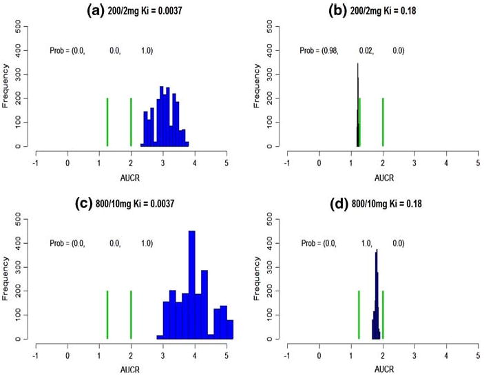
Population average DDI prediction. The green bars cut the axis into three intervals, (– ∞, 1.25), (1.25, 2), (2, ∞). The probabilities on the top represent the probabilities falling into these intervals. a–d The predicted population average DDI at various dose combinations and K_i

With a much higher dose combination, 800/10 mg, a K_i of 0.18 leads to a predicted AUCR_pop = 1.78 ×/÷ 1.027 (Table 3). Its probabilities in three intervals are (0.0, 1.0, 0.0) (Fig. 2d), and the inhibition is concluded as a weak one. On the other hand, for a much smaller K_i, 0.0037, AUCR_pop is predicted as 3.93 ×/÷ 1.14 with probabilities, (0.0, 0.0, 1.0) (Fig. 2c), and inhibition is concluded to be both statistically and clinically significant.

Fig. 2.

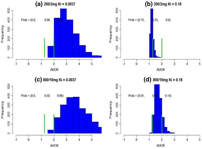
Subject-specific DDI prediction. The green bars cut the axis into three intervals, (– ∞, 1.25), (1.25, 2), (2, ∞). The probabilities on the top represent the probabilities falling into these intervals. a–d The predicted subject-specific DDI at various dose combinations and K_i

Subject-specific DDI prediction

Providing a 200/2 mg KETO/MDZ dose combination, the predicted AUCR_subj based on between-subject variation is from 1.19 ×/÷ 1.084 to 2.95 ×/÷ 1.26 for K_i of 0.18 and 0.0037, respectively (Table 4). Its probabilities in three intervals are (0.75, 0.25, 0.0) and (0.0, 0.06, 0.94), respectively (Fig. 2a, b). Therefore, K_i = 0.18 will lead to a weak DDI conclusion, and K_i = 0.0037 will lead to a statistically and clinically significant DDI. Given a much higher dose combination, 800/10 mg, a K_i of 0.18 leads to a predicted AUCR_subj = 1.69 ×/÷ 1.15 (Table 4). Its probabilities in three intervals are (0.01, 0.85, 0.14) (Fig. 3d), and the inhibition is concluded as a weak one. On the other hand, for a much smaller K_i, 0.0037, AUCR_subj is predicted as 3.61 ×/÷ 1.28 with probabilities, (0.0, 0.02, 0.98) (Fig. 3c), and inhibition is concluded both statistically and clinically significant.

Table 4.

Subject-specific average DDI prediction

Ki	KETO (mg)/MDZ (mg)
	200/2	800/10
0.18	1.19 ×/÷ 1.084	1.69 ×/÷ 1.15
0.0037	2.95 ×/÷ 1.26	3.61 ×/÷ 1.28

Geometric mean ×/÷ (1 + CV) of the predicted AUCR

Fig. 3.

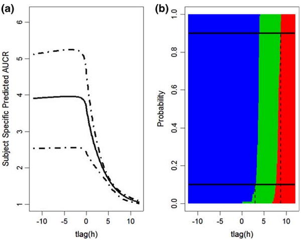
Effects of dosage separation on DDI when KETO(PO)/MDZ(IV) combination is 800/10 mg and K_i = 0.0037. a The mean and 90% credit intervals for AUCR predicted based on between-subject variability across the interval from −12 to 12 h. Negative values indicate that KETO is administrated before MDZ, and positive that MDZ administered prior to KETO. b The blue represents Pr{AUCR_subj > 2}, the green represents Pr{1.25 < AUCR_subj < 2}, the red represents Pr{AUCR_subj < 1.25}. The top black solid horizontal line represents the probability = 0.9, and it crosses the red region when the interval between administration is 8.8, indicating that if PO KETO is administrated 8.8 h after MDZ IV or later, the effect on AUCR will be clinically insignificant with probability larger that 90%. The black solid line at the bottom represents probability = 0.1, and it crosses the blue region when the time interval between dosage of interacting drugs is 3.0, meaning that if PO KETO is administrated within 3 h after MDZ IV, the inhibition will be clinically significant with probability larger that 90%. Otherwise, their DDI will be a weak interaction

The effect of dosing interval on KETO/MDZ interaction

Administration of the KETO PO dose (800 mg) was simulated from 12 h before to 12 h after the MDZ IV dose (10 mg), with K_i set at 0.0037. According to the previous analysis, simultaneous KETO/MDZ interaction showed the highest interaction based on this dose and K_i combination. Figure 3a presents the relationship between the time between KETO and MDZ doses and predicted subject-specific level AUCR. The solid line is AUCR_subj, and the dashed lines are its 95% credit intervals. The maximum AUCR_subj happens when KETO is administrated about 4.5 h before MDZ, AUCR_subj = 4.02 ×/÷ 1.31. At the mean level, this is 11% greater than the AUCR_subj when the drugs are administered simultaneously, 3.61 ×/÷ 1.28.

If KETO is administrated after MDZ, its inhibition effect is quickly diminished. In order to tell the probabilities of AUCR_subj falling into three DDI intervals, they are displayed in a heatmap (Fig. 3b). The blue represents Pr{AUCR_subj > 2}, the green represents Pr{1.25 < AUCR_subj < 2}, the red represents Pr{AUCR_subj < 1.25}, with these probabilities represented across the differences in dosing times. The top black solid horizontal line represents the probability = 0.9, and it crosses the red region when KETO is administered 8.8 h after MDZ. Thus, if PO KETO is administrated more than 8.8 h after MDZ IV, their inhibition will be clinically insignificant with probability larger that 90%. The black solid line at the bottom of Fig. 3 represents a probability = 0.1 and intersects the blue region at +3.0 h, indicating that if PO KETO is administrated before or within 3 h after MDZ IV, it will cause a clinically significant reduction in MDZ clearance with probability greater that 90%. Otherwise, their DDI will be a weak interaction.

The effect of KETO formulation and food on subject specific AUCR prediction

Published KETO PK studies used to develop the model [8, 9] utilized various KETO formulations and conditions: tablet fasting (TF), tablet with a meal (TM), suspension fasting (SPF), solution with a meal (SLM), and solution fasting (SLF), respectively. The corresponding ka posterior distributions were estimated from published sample mean data. The effects of food and formulation on the predicted AUCR_subj are displayed in Fig. 4. When KETO/MDZ dose combination is 800/10 mg and K_i = 0.0037, they all have similar distributions, and the probabilities in three DDI intervals are very similar.

Fig. 4.

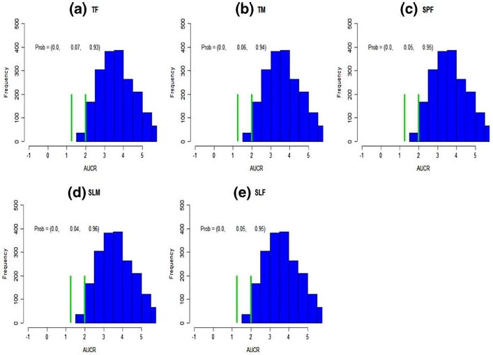
The effect of KETO administration route on AUCR. Predictions incorporated individual subject variability. The notations (TF, TM, SPF, SLM, SLF) represent tablet fasting (a), tablet meal (b), suspension fasting (c), solution meal (d), and solution fasting (e), respectively. The KETO(PO)/MDZ(IV) combination is 800/10 mg and K_i = 0.0037

Discussion

An innovative probabilistic rule is proposed to predict the clinical significance or clinical insignificance of DDI. A KETO/MDZ inhibition combination is used as an example. This rule can be applied to predictions of both population-average and subject-specific level AUCR's to determine the extent of a DDI. As shown, AUCR_subj prediction always exhibit larger variances than the corresponding AUCR_pop. Hence, a clinically insignificant AUCR_pop is not necessarily true when considering between-subject variability. For example, under the 200/2 mg KETO/MDZ dose combination and a K_i = 0.18, the population-average DDI claim an insignificant KETO/MDZ interaction (Fig. 1b). On the other hand, its subject-specific level prediction is concluded as a weak DDI (Fig. 2b).

It is very clear that AUCR highly depends on the K_i and dose combination chosen. Simulations were run with K_i set at 0.0037 or 0.18 μM, the values set forth in the FDA Guidance (http://www.fda.gov/cder/guidance/6695dft.pdf). This nearly 50-fold range in the in vitro K_i values can greatly impact the conclusion of DDI significance. This variability may arise from different buffer conditions, the enzyme source, and the concentration of substrate and inhibitor studied. Hepatocyte and microsomal studies may yield different results as hepatocytes require that the drug access an intact cell system [15]. Standardization and optimization of the in vitro assay to determine K_i is necessary to accurately predict DDI potential of a new compound. Similarly, the design of the clinical trial can influence the effect of the DDI. The trial should be designed to determine the “worst-case scenario,” i.e. doses of KETO and MDZ should be administered at a time when maximal inhibition is likely to occur. As shown in Fig. 4, KETO administered 4.5 h before MDZ would result in the maximal interaction.

The main advantage of probabilistic rule to predict clinical significance of DDI over the deterministic rule is that the probabilistic rule considers the sample variations, while deterministic rule does not. For example, for a dose combination 200/2 mg and K_i = 0.18 μM, predicted AUCR_subj is 1.19 ×/÷ 1.084 and its probabilities in the three intervals are 0.75, 0.25, 0.0. Based on this, it is classified as a weak inhibitor. However, if it is judged under the deterministic rule, 75% of time it will be declared insignificant inhibition, and 25% of time it will claimed to be a weak inhibitor.

We utilized a hierarchical Bayesian meta-analysis model designed to summarize published sample mean and sample variance data [8, 9]. It is capable of recovering between subject and between study variances. Information from these recovered variances information became the foundation for the AUCR prediction at the subject level. On the other hand, if the data from original PK studies are available with PK parameters for each individual, many conventional Bayesian PK models can be applied [16–21].

There are several limitations in the MDZ/KETO model that we applied to illustrate our probabilistic rule. For instance, the current MDZ model (2) assumes that 100% of clearance is by hepatic CYP3A. However, approximately 10% of MDZ's clearance is through non-CYP3A mechanisms. Incorporating non-inhabitable elimination will reduce the extent of the DDI. These models also assume that the concentration of substrate (MDZ) and inhibitor (KETO) at the active site is equivalent to the concentration in the central compartment. A potentially higher active site concentration of KETO will lead to a larger AUCR. This paper only considers the inhibition of MDZ administered by IV route. A similar model for PO MDZ is more complex as it would need to incorporate information on inhibition of CYP3A in the intestine. The model does not take any correlation between the PK of MDZ and KETO for an individual person into account. While we recognize that the CL of the two drugs may be related, e.g. to body weight or genotype, we do not currently have the information required to build this correlation into our model.

While we utilized our Bayesian MCMC model to estimate between-subject variability in PK parameters, the probabilistic rule proposed in this paper may be applied to any situation in which the individual PK models, incorporating variability, are available for both the inhibitor and substrate. It fits well with newly developed FDA guidelines for exploratory IND studies (http://www.fda.gov/cder/ guidance/6695dft.pdf). This document highly recommends a PK study of an investigational drug at a very low dosing level and of a short duration. The purpose is to obtain this drug's PK, instead of investigating its pharmacologic effects. If this investigational drug is an inhibitor, its PK data and model may be incorporated with PK data that is available for many common substrates and the K_i values determined in vitro for the substrate-inhibitor combination. The interaction potential of this new agent can thus be predicted at both subject-specific and population-average levels. This same strategy can be applied to a new compound that is a substrate by nature, utilizing PK data for the enzyme inhibitor (e.g. KETO). If one is able to predict either a clinically significant or insignificant DDI with probability greater than 90%, no further in vivo DDI study may be required. Only when predicted as a weak DDI, a further in vivo DDI may be required to assess the clinical extent of the interaction. In these cases, utilizing the predictive PK interaction model may enhance the design of a trial to determine a DDI. As shown in Fig. 3, the time interval between administration of inhibitor and substrate may impact the AUCR.

If a drug's in vivo pharmacokinetics variability isn't available, they can be built up with data known for drugs in the same class, or information on enzyme variability (e.g. genetic variation), or variability seen in vitro (e.g. in hepatocytes obtained from different individuals). This bottom-up strategy is described in the literature [22]. The challenge of this approach is to establish and validate the equivalence between predicted DDI variability and clinical DDI variability.

The probabilistic decision rule presented here provides an alternative to the deterministic rule commonly utilized. This novel method takes into account stochastic variability in the determination of a clinically significant DDI. While DDI may be predicted using both population-average and subject-specific data, we recommend subject-specific DDI prediction since it contains more information on variation across the population.

Appendix

Meta-analysis models for individual level data

When individual level data are available for each study, summarizing PK parameters from multiple sources by meta-analysis has been addressed by applying Bayesian methods to construct a drug PK model from several clinical study data sets. (See, e.g. Wakefield and Rahman [20]). In general, the following set of models are used

• subject-specific PK model:

  $$\left[y_{\text{mjkh}}|{\beta }_{\text{mk}},z_{\text{jkh}}\right]\sim \text{MVN}\left[f\left({\beta }_{\text{mk}},z_{\text{jkh}}\right),{\sigma }_0^2\right],$$ (13)

• subject-specific PK parameter model in study k:

  $$\left[{\beta }_{\text{mk}}|{\beta }_k,\sum \right]\sim \text{MVN}({\beta }_k,\sum ),$$ (14)

• study-specific PK parameter model:

  $$\left({\beta }_k|\beta ,\Omega \right)\sim \text{MVN}(\beta ,\Omega )$$ (15)

In (13), y_mjkh represents log-transformed drug concentration at time t_jkh for subject m in phase h of study k. Here we use a generic notation z_jkh to denote available data and constants for a study subject at time t_jkh. It includes dosage, dosing route, and fixed constants such as Q_h, F_I, Km_I, fu_I, MW_I, Km_S, fu_S, and time point t_jkh at which plasma concentration is measured. The mean value f(β_mk, z_jkh) is the predicted log-transformed drug concentration for subject m at jth time point from phase h of study k. In the case that y_mjkh is the KETO concentration observed from the first compartment, then f(β_mk, z_jkh) = log(A1_I/V1_I). The measurement error variation, ${\text{σ}}_0^2$, is assumed equal across studies. The variance components Σ and Ω are for subject-specific and study-specific PK parameters.

However, published data are often available in the form of sample average plasma concentration. In other words, only $({\overline{y}}_{•\text{jkh}},S_{\text{jkh}}^2)$, instead of y_ijkh are published. But model (13) obviously needs y_mjkh, and hence cannot be directly implemented to perform meta-analysis with summarized data. Reconstructing a drug PK model from $({\overline{y}}_{•\text{jkh}},S_{\text{jkh}}^2)$ needs a new meta-analysis formulation and different Bayesian sampling algorithm.

Meta-analysis models with sample mean and standard deviation data

As individual data are not available, it is an unrealistic goal to estimate subject level PK parameters. The sample mean data ȳ_•jkh at most provide information about study specific PK parameters β_k and study to study variation parameters Ω. The sample variance data ${\text{S}}_{\text{jkh}}^2$ at most provide information about between-subject heterogeneity parameter Σ. As a result, models based on (13)–(15) are only suitable when working on subject level data. When only sample mean and sample variance data are available, they need to be modified to make estimation feasible. In other words, the models should not involve β_mk. A natural approach is to base estimation methods on marginalized likelihood where β_mk is integrated out. However, as no analytic form is available for f(β_mk, z_jkh), direct integration is not feasible. The alternative we take is to first derive an approximation for f(β_mk, z_jkh) and then marginalize. Specifically, we adapt as follows.

By Taylor expansion at β_k, f(β_mk, z_jkh) can be approximated as

$$f\left({\beta }_{\text{mk}},z_{\text{jkh}}\right)\approx f\left({\beta }_k,z_{\text{jkh}}\right)+{\left(\frac{\partial f}{\partial {\beta }_{\text{mk}}}{|}_{{\beta }_{\text{mk}}={\beta }_k}\right)}^T\left({\beta }_{\text{mk}}-{\beta }_k\right).$$ (16)

Denote $F_{\text{jkh}}=\frac{\partial f}{\partial {\beta }_{\text{mk}}^T}{|}_{{\beta }_{\text{mk}}={\beta }_k}$. Instead of individual level PK model (16), we assume the following approximated model $\left[y_{\text{mjkh}}|{\beta }_{\text{mk}},{\beta }_k,{\sigma }_0^2,z_{\text{jkh}}\right]\sim N(f\left({\beta }_k,z_{\text{jkh}}\right)+F_{\text{jkh}}^T\left({\beta }_{\text{mk}}-{\beta }_k\right),{\sigma }_0^2$. Now by integrating out β_mk using the conditional distribution of β_mk given β_k, we have

$$\left[y_{\text{mjkh}}|{\beta }_k,z_{\text{jkh}},\sum ,{\sigma }_0^2\right]\sim N\left(f\left({\beta }_k,z_{\text{jkh}}\right),F_{\text{jkh}}^T\sum F_{\text{jkh}}+{\sigma }_0^2\right)$$ (17)

As a result,

$$\left[{\overline{y}}_{•\text{jkh}}|{\beta }_k,z_{\text{jkh}},\sum ,{\sigma }_0^2\right]\sim N\left(f\left({\beta }_k,z_{\text{jkh}}\right),\frac{F_{\text{jkh}}^T\sum F_{\text{jkh}}+{\sigma }_0^2}{n_{\text{kh}}}\right)$$ (18)

To obtain the approximate distribution for sample variance, $S_{\text{jkh}}^2={\sum }_{i=1}^{n_{\text{kh}}}{\left(y_{\text{ijkh}}-{\overline{y}}_{•\text{jkh}}\right)}^2/\left(n_{\text{kh}}-1\right)$, we use the known fact the normalized sample variance of m i.i.d. normal variables has a Chi-square distribution with degree of freedom m – 1. From the approximate model (18), we immediately obtain

$$\frac{{{\sum }_{i=1}^{n_{h_k}}\left(y_{\text{mjkh}}-{\overline{y}}_{•\text{jkh}}\right)}^2}{F_{\text{jkh}}^T\sum F_{\text{jkh}}+{\sigma }_0^2}\sim {\chi }_{n_{\text{kh}}-1,}^2\text{or equivalently},\frac{\left(n_{\text{kh}}-1\right)}{F_{\text{jkh}}^T\sum F_{\text{jkh}}+{\sigma }_0^2}{S}_{\text{jkh}}^2\sim {\chi }_{n_{\text{kh}}}^2-1$$ (19)

Notice that (18) and (19) depend only on β_k, Σ, and ${\sigma }_0^2$. Hence estimation of these parameters is feasible with mean and standard deviation data. Our estimation will be based on the following hierarchical models.

• Sample mean PK model

  $$\left[{\overline{y}}_{•\text{jkh}}|{\beta }_k,z_{\text{jkh}},\sum ,{\sigma }_0^2\right]\sim N\left(f\left({\beta }_k,z_{\text{jkh}}\right),\frac{F_{\text{jkh}}^T\sum F_{\text{jkh}}+{\sigma }_0^2}{n_{\text{kh}}}\right)$$ (20)

• Sample variance PK model

  $$\frac{\left(n_{\text{kh}}-1\right)}{F_{\text{jkh}}^T\sum F_{\text{jkh}}+{\sigma }_{\text{0}}^2}{S}_{\text{jkh}}^2\sim {\chi }_{n_{\text{kh}}-1}^2$$ (21)

• Study-specific PK parameter model:

  $$\left[{\beta }_k|\beta ,\Omega \right]\sim \text{MVN}\left(\beta ,\Omega \right)$$ (22)

Many times, a main purpose of determining variability is to identify individuals at risk. However as our model is based on summarized data, no individual information is available. All we can do is to quantify variance for a given population. Of course if individual data are available, subject covariates can be used in explaining variability using individual level models.

Prior specification and posterior distributions

$$\begin{array}{l}p\left(\beta \right)=U\left(0,{10}^4\right)\\ p\left({\sigma }_l^2\right)=U\left(a,b\right)\iff p\left({\sigma }_l^{-2}\right)=\frac{{\left({\sigma }_l^{-2}\right)}^{-2}}{\left(b-a\right)},l=0,1,\dots ,q;\\ p\left({\omega }_l^2\right)=U\left(a,b\right)\iff p\left({\omega }_l^{-2}\right)=\frac{{\left({\omega }_l^{-2}\right)}^{-2}}{\left(b-a\right)},l=1,\dots ,q.\end{array}$$ (23)

Variance components all follow a uniform prior because practically they rarely exceed the bound (a, b) = (0.01², 2²). Let Ȳ• = {Ȳ_•jkh; j = 1,…, T_kh; k = 1,…, K; h = 1,…, H_k} be the sample mean data and $S=\left\{S_{\text{jkh}}^2;j=1,\dots ,T_{\text{kh}};k=1,\dots ,K;h=1,\dots ,H_k\right\}$ the sample variance data. Then, the posterior probability distribution based on (20)–(22) and priors (23) is,

$$\begin{array}{l}p\left({\beta }_1,\dots ,{\beta }_K,\sum ,\Omega ,{\sigma }_0^2|{\overline{Y}}_{•},S,z\right)\\ \propto \left\{\prod _{k=1}^K\prod _{h=1}^{H_k}\prod _{j=1}^{T_{\text{kh}}}N({\overline{y}}_{•\text{jkh}}\left|f\right({\beta }_k,t_{\text{jkh}}),\frac{F_{\text{jkh}}^T\sum F_{\text{jkh}}+{\sigma }_0^2}{n_{\text{kh}}}\right)\}\\ \times \left\{\prod _{k=1}^K\prod _{h=1}^{H_k}\prod _{j=1}^{T_{\text{kh}}}{\chi }_{n_{h_k}-1}^2\left(\frac{\left(n_{\text{kh}}-1\right)S_{\text{jkh}}^2}{F_{\text{jkh}}^T\sum F_{\text{jkh}}+{\sigma }_0^2}\right)\right\}\\ \times \left\{\prod _{k=1}^{K}p\left({\beta }_k|\beta ,\Omega \right)\right\}\times p\left(\beta \right)\times p\left(\sum \right)\times p(\Omega )\times p\left({\sigma }_0^2\right)\end{array}$$ (24)

The estimation procedure is implemented with a Monte Carlo Markov chain method. The posterior probability functions, $p\left(\beta |•\right),p\left({\beta }_k|•\right),p\left({\sigma }_0^{-2}|•\right),p\left({\sigma }_l^{-2}|•\right),\text{and}p\left({\omega }_0^{-2}|•\right)$ are derived in the following.

$$p({\beta }_l|•)\propto \left\{\prod _{h=1}^{H_k}\prod _{j=1}^{T_{\text{kh}}}N\left(f(\alpha ,{\beta }_k,z_{\text{jkh}}),\frac{F_{\text{jkh}}^T\sum F_{\text{jkh}}+{\sigma }_{0k}^2}{n_k}\right)\right\}\times \left\{\prod _{k=1}^{K}p({\beta }_k|\beta ,\Omega )\right\}$$ (25)

$$p({\beta }_l|•)\propto N\left({\left\{\frac{1}{{\tau }_l^2}+\frac{K}{{\omega }_l^2}\right\}}^{-1}\left\{\frac{1}{{\tau }_l^2}{\mu }_l+\frac{K}{{\omega }_l^2}{\overline{\beta }}_{•l}\right\},{\left\{\frac{1}{{\tau }_l^2}+\frac{K}{{\omega }_l^2}\right\}}^{-1}\right)$$ (26)

for l = 1,…,q; where $\overline{\beta }{.}_l={\sum }_{K=1}^K{\beta }_{\text{kl}}$ Variance components:

$$\text{Pr}\left({\omega }_l^2|•\right)\sim \text{Inv}-\text{Gamma}\left[\left(\frac{K}{2}-1\right),\left(\frac{{{\sum }_{k=1}^k\left({\beta }_{\text{kl}}-{\beta }_l\right)}^2}{2}\right)\right]\times 1_{{\omega }_l^2}({0.01}^2,2^2)$$ (27)

where $1_{{\omega }_l^2}$ (0.01²,2²) equals 1 when ${\omega }_l^2$ is inside (0.01², 2²) and 0 otherwise.

$$\begin{array}{l}p\left({\sigma }_1^2\right|•)\propto \prod _{k=1}^K\prod _{h=1}^{H_k}\prod _{j=1}^{T_{\text{kh}}}{(F_{\text{jkh}}^T{F}_{\text{jkh}}{\sigma }_1^2+{\sigma }_0^2)}^{-\frac{n_{\text{kh}}}{2}+1}\\ \times \text{exp}\left\{-\frac{n_{\text{kh}}{\left\{{\overline{y}}_{•\text{jkh}}-f\left(\alpha ,{\beta }_k,z_{\text{jkh}}\right)\right\}}^2+{\sum }_{i=1}^{n_{\text{kh}}}{\left(y_{\text{ijkh}}-{\overline{y}}_{•\text{jkh}}\right)}^2}{2\left(F_{\text{jkh}}^T{F}_{\text{jkh}}{\sigma }_1^2+{\sigma }_0^2\right)}\right\}\\ \times 1_{{\sigma }_1^2}\left({0.01}^2,2^2\right)\end{array}$$ (28)

$$\begin{array}{l}p\left({\sigma }_1^2\right|•)\propto \prod _{k=1}^K\prod _{h=1}^{H_k}\prod _{j=1}^{T_{\text{kh}}}{(F_{\text{jkh}}^T{F}_{\text{jkh}}{\sigma }_1^2+{\sigma }_0^2)}^{-\frac{n_{\text{kh}}}{2}+1}\\ \times \text{exp}\left\{-\frac{n_{\text{kh}}{\left\{{\overline{y}}_{•\text{jkh}}-f\left(\alpha ,{\beta }_k,z_{\text{jkh}}\right)\right\}}^2+{\sum }_{i=1}^{n_{\text{kh}}}{\left(y_{\text{ijkh}}-{\overline{y}}_{•\text{jkh}}\right)}^2}{2\left(F_{\text{jkh}}^T{F}_{\text{jkh}}{\sigma }_1^2+{\sigma }_0^2\right)}\right\}\\ \times 1_{{\sigma }_1^2}\left({0.01}^2,2^2\right)\end{array}$$ (29)

Here $1_{{\text{σ}}_1^2}$ (0.01²,2²) and $1_{{\sigma }_0^2}$ (0.01²,2²) are similarly defined as $1_{{\omega }_{\mathrm{l}}^2}$ (0.01²,2²).

MCMC convergence

Samples are drawn through the Metropolis Hasting (MH) algorithm (Hastings et al. 1970). At each step, a random walk chain is used and the random perturbation is taken to mean normal with mean 0 and standard deviation of 10%. The mixing is well with such proposed density and the acceptance rate varies. For most of the study specific parameters β_k, the acceptance rates are close to 25%. Five independent chains were run simultaneously to determine the convergence with dispersed starting values on population parameters. It needed less than 4000 iterations for the estimated potential scale reduction criterion of Gelman and Rubin [23] to be less than 1.2. By visual inspection of trace plots, almost all chains start to mix well after 500 iterations. The final results are based on a single chain of 50,000 iterations after a burn-in of 10,000. Every tenth iteration after burn-in was extracted for summarizing results.

References

- 1.Monahan BP, Ferguson CL, Killeavy ES, Lloyd BK, Troy J, Cantilena LR., Jr Torsades de pointes occurring in association with terfenadine use. JAMA. 1990;264(21):2788–2790. [PubMed] [Google Scholar]
- 2.Watabe T. Strategic proposals for predicting drug-drug interactions during new drug development: based on sixteen deaths caused by interactions of the new antiviral sorivudine with 5-fluorouracil prodrugs. J Toxicol Sci. 1996;21(5):299–300. doi: 10.2131/jts.21.5_299. [DOI] [PubMed] [Google Scholar]
- 3.Okuda H, Nishiyama T, Ogura K, Nagayama S, Ikeda K, Yamaguchi S, Nakamura Y, Kawaguchi Y, Watabe T. Lethal drug interactions of sorivudine, a new antiviral drug, with oral 5-fluorouracil prodrugs. Drug Metab Dispos. 1997;25(5):270–273. [PubMed] [Google Scholar]
- 4.Ito K, Iwatsubo T, Kanamitsu S, Ueda K, Suzuki H, Sugiyama Y. Prediction of pharmacokinetic alterations caused by drug-drug interactions: metabolic interaction in the liver. Pharmacol Rev. 1998;50(3):387–412. [PubMed] [Google Scholar]
- 5.Ito K, Iwatsubo T, Kanamitsu T, Nakajima S, Sugiyama Y. Quantitative prediction of in vivo drug clearance and drug interactions from in vitro data on metabolism, together with binding and transport. Annu Rev Pharmacol Toxicol. 1998;38:461–499. doi: 10.1146/annurev.pharmtox.38.1.461. [DOI] [PubMed] [Google Scholar]
- 6.Yang J, Kjellsson M, Rostami-Hodjegan A, Tucker GT. The effects of dose staggering on metabolic drug-drug interactions. Eur J Pharm Sci. 2003;20(2):223–232. doi: 10.1016/s0928-0987(03)00200-8. [DOI] [PubMed] [Google Scholar]
- 7.Ito K, Chiba K, Horikawa M, Ishigami M, Mizuno N, Aoki J, Gotoh Y, Iwatsubo T, Kanamitsu S, Kato M, Kawahara I, Niinuma K, Nishino A, Sato N, Tsukamoto Y, Ueda K, Itoh T, Sugiyama Y. Which concentration of the inhibitor should be used to predict in vivo drug interactions from in vitro data? AAPS Pharmsci. 2002;4(4):E25. doi: 10.1208/ps040425. [DOI] [PMC free article] [PubMed] [Google Scholar]
- 8.Li L, Yu M, Chin R, Lucksiri A, Flockhart D, Hall DS. Drug–drug Interaction prediction: a Bayesian meta-analysis approach. Stat Med. 2007;26(20):3700–3721. doi: 10.1002/sim.2837. [DOI] [PubMed] [Google Scholar]
- 9.Yu M, Kim S, Wang Z, Hall DS, Li L. A Bayesian meta-analysis on published sample mean and variance pharmacokinetic data with application to drug–drug interaction prediction. J Biopharm Stat. 2007 doi: 10.1080/10543400802369004. in press. [DOI] [PMC free article] [PubMed] [Google Scholar]
- 10.Tsunoda SM, Velez RL, von Moltke LL, Greenblatt DJ. Differentiation of intestinal and hepatic cytochrome P450 3A activity with use of midazolam as an in vivo probe: effect of ketoconazole. Clin Pharmacol Ther. 1999;66(5):461–471. doi: 10.1016/S0009-9236(99)70009-3. [DOI] [PubMed] [Google Scholar]
- 11.Cleary JD, Taylor JW, Chapman SW. Itraconazole in antifungal therapy. Ann Pharmacother. 1992;26(4):502–509. doi: 10.1177/106002809202600411. [DOI] [PubMed] [Google Scholar]
- 12.Price PS, Conolly RB, Chaisson CF, Gross EA, Young JS, Mathis ET, Tedder DR. Modeling interindividual variation in physiological factors used in PBPK models of humans. Crit Rev Toxicol. 2003;33(5):469–503. [PubMed] [Google Scholar]
- 13.Martinez-Jorda R, Rodriguez-Sasianin JM, Calvo R. Serum binding of ketoconazole in health and disease. Int J Clin Pharmacol Res. 1990;5:271–276. [PubMed] [Google Scholar]
- 14.Rowland M, Tozer TN. Clinical pharmacokinetics concept and applications. 3rd. Lippincott Williams & Wilkins; London: 1995. [Google Scholar]
- 15.Van L, Heydari A, Yang J, Hargreaves J, Rowland-Yeo K, Lennard MS, Tucker GT, Rostami-Hodjegan A. The impact of experimental design on assessing mechanism-based inactivation of CYP2D6 by MDMA (Ecstasy) J Psychopharmacol. 2006;20:834–841. doi: 10.1177/0269881106062902. [DOI] [PubMed] [Google Scholar]
- 16.Wakefield JC, Smith AFM, Racine-Poon A, Gelfand AE. Bayesian analysis of linear and non-linear population models by using the Gibbs sampler. Appl Stat. 1994;43:201–221. [Google Scholar]
- 17.Wakefield JC. Bayesian individualization via sampling-based methods. J Pharmacokinet Biopharm. 1996;24(1):103–131. doi: 10.1007/BF02353512. [DOI] [PubMed] [Google Scholar]
- 18.Wakefield JC. The Bayesian analysis of population pharmacokinetic models. J Am Stat Assoc. 1996;91:62–75. [Google Scholar]
- 19.Wakefield JC, Bennett JE. The Bayesian modeling of covariates for population pharmacokinetic models. J Am Stat Assoc. 1996;91:917–927. [Google Scholar]
- 20.Wakefield JC, Rahman N. The combination of population pharmacokinetic studies. Biometrics. 2000;56(1):263–270. doi: 10.1111/j.0006-341x.2000.00263.x. [DOI] [PubMed] [Google Scholar]
- 21.Lopes HF, Muller P, Rosner GL. Bayesian meta-analysis for longitudinal data models using multivariate mixture priors. Biometrics. 2003;59(1):66–75. doi: 10.1111/1541-0420.00008. [DOI] [PubMed] [Google Scholar]
- 22.Rostami-Hodjegan A, Tucker G. “In Silico” simulations to assess the “in vivo” consequences of “in vitro” metabolic drug-drug interactions. Drug Discov Today Technol. 2004;1:441–448. doi: 10.1016/j.ddtec.2004.10.002. [DOI] [PubMed] [Google Scholar]
- 23.Gelman A, Rubin DB. Inference from iterative simulation using multiple sequences. Stat Sci. 1992;7:457–472. [Google Scholar]
- 24.Gascoigne EW, Barton GJ, Michaels M, Meuldermans W, Heykans J. The kinetics of ketoconazole in animals and man. Clin Res Rev. 1991;1(3):177–187. [Google Scholar]
- 25.Daneshmend TK, Warnock DW, Turner A, Roberts CJ. Pharmacokinetics of ketoconazole in normal subjects. J Antimicrob Chemother. 1981;8:299–304. doi: 10.1093/jac/8.4.299. [DOI] [PubMed] [Google Scholar]
- 26.Daneshmend TK, Warnock DW, Ene MD, Johnson EM, Parker G, Richardson MD, Roberts CJ. Multiple dose pharmacokinetics of ketoconazole and their effects on antipyrine kinetics in man. J Antimicrob Chemother. 1983;12(2):185–188. doi: 10.1093/jac/12.2.185. [DOI] [PubMed] [Google Scholar]
- 27.Daneshmend TK, Warnock DW, Ene MD, Johnson EM, Potten MR, Richardson MD, Williamson PJ. Influence of food on the pharmacokinetics of ketoconazole. Antimicrob Agents Chemother. 1984;25(1):1–3. doi: 10.1128/aac.25.1.1. [DOI] [PMC free article] [PubMed] [Google Scholar]
- 28.Huang YC, Colaizzi JL, Bierman RH, Woestenborghs R, Heykants J. Pharmacokinetics and dose proportionality of ketoconazole in normal volunteers. Antimicrob Agents Chemother. 1986;30(2):206–210. doi: 10.1128/aac.30.2.206. [DOI] [PMC free article] [PubMed] [Google Scholar]
- 29.Lee JI, Chaves-Gnecco D, Amico JA, Kroboth PD, Wilson JW, Frye RF. Application of semisimultaneous midazolam administration for hepatic and intestinal cytochrome P450 3A phenotyping. Clin Pharmacol Ther. 2002;72(6):718–728. doi: 10.1067/mcp.2002.129068. [DOI] [PubMed] [Google Scholar]