Abstract
Many biomedical problems relate to mutant functional properties across a sequence space of interest, e.g., flu, cancer, and HIV. Detailed knowledge of mutant properties and function improves medical treatment and prevention. A functional census of p53 cancer rescue mutants would aid the search for cancer treatments from p53 rescue. We devised a general methodology for conducting a functional census of a mutation sequence space, and conducted a double-blind predictive test on the functional rescue property of 71 novel putative p53 cancer rescue mutants iteratively predicted in sets of 3. Double-blind predictive accuracy (15-point moving window) rose from 47% to 86% over the trial (r = 0.74). Code and data are available upon request1.
Keywords: Biology and genetics, Feature extraction or construction, Machine learning, Medicine and science
1 Introduction
Mutations and their functional effects drive evolution, drug resistance, genetic disorders, viral evasion of the immune system, and other important biomedical processes. In pharmacogenomics [1] and drug resistant HIV [2],[3],[4], detailed knowledge of functionally important mutations leads directly to better patient treatment. In flu [5], knowledge of important mutations leads directly to better disease prevention, by way of better vaccine design. In cancer, the concern of this paper, the effect of functionally important mutations causes the disease.
Medical practice is often advanced by knowing mutant functional properties across a mutation sequence space of specific interest. One difficulty is that mutation spaces grow to be combinatorially large, while experimental time and resources remain bounded. Computational analysis is challenging because subtle effects on structure and function result in broad and diverse changes.
1.1 p53 overview
Cancer is caused by the accumulation of genetic mutations in two critical regulatory pathways: normal cell growth, and programmed cell death (apoptosis). Defects in the cell growth pathway can result in uncontrolled cellular proliferation. Tumor suppressor proteins such as p53 normally trigger apoptosis in affected cells and destroy the tumor.
p53 exerts its tumor suppressor activity mainly as a transcription factor that induces cell cycle arrest, apoptosis, DNA repair, and/or senescence. It is stabilized and activated in response to cell stress by a complicated series of post-translational modifications [6],[7],[8],[9]. Activated p53 suppresses tumors through one of the following mechanisms:
Induction – p53 directly targets and induces genes with tumor supressor functions [10],[11]. There are approximately 100 known genes with p53 binding sites [12], and several hundred genes are directly or indirectly upregulated by activated p53 [13] ,[14].
Repression – p53 also represses the expression of genes. As most of the repressed genes lack a distinct p53 binding site the mechanism is currently unknown [15].
Non-transcriptional Mechanisms – p53 translocates to the mitochondria in response to DNA damage and causes cytochrome c release [16],[17].
p53 mutations that disrupt these mechanisms are complicit in human cancers. The International Agency for Research on Cancer (IARC) TP53 Mutation Database2 (R10) lists 21,588 p53 mutations found in human cancer patients [18]. 71% of the entries (15,387) result in full-length protein with a single amino acid change in the DNA binding p53 core domain. The top eight mutants account for 30% and the top 50 account for 54% of these single amino acid change mutants [19].
The structure of full-length wild-type p53 is unknown, but the crystal structure of the core domain [20], in conjunction with biophysical and NMR studies [21],[22],[23], has made it possible to construct homology models. p53 has 393 amino acids and three important domains: an amino-terminal transactivation domain, a core domain consisting of amino acids 96−292 which recognizes p53 DNA binding sites, and a carboxy-terminal tetramerization domain [24],[25],[26],[27],[28].
1.2 Novel cancer treatments and p53 functional rescue
A long-held medical goal for anti-cancer therapy is achieving functional rescue of p53 cancer mutants by stabilizing the wild-type conformation, thereby activating apoptosis in cancerous cells and shrinking or killing the tumor. Several promising drug-like small molecules have been identified [29],[30], but their mechanisms of action and their spectra of activity are not known. This has led to intense scientific interest in the basic mechanisms of p53 functional rescue.
1.2.1 p53 cancer rescue mutants
We established the existence of global functional rescue mechanisms for p53 cancer mutants [31] through studies of intragenic second-site suppressor mutations that restore native p53 function (“cancer rescue,” “cancer suppressor,” among other names). Surprisingly, a second-site p53 suppressor mutation can co-occur with a p53 cancer mutation such that functional effects cancel and the double mutant protein has normal p53 function.
A search for such suppressor mutations resulted in identification of a “global suppressor motif” involving core domain amino acids 235, 239 and 240 [32]. Specific amino acid changes of one or more of these restored p53 function to 16 of 30 of the most common p53 cancer mutants tested.
1.2.2 Terminology
In this paper, the terms active and inactive are used to describe mutant functionality. In other literature an active mutant may be referred to as a “functional,” “positive,” or “rescued” mutant and an inactive mutant may be referred to as a “non-functional,” “negative,” or “cancer” mutant.
1.3 Computational approaches to p53
The p53 mutant classification problem is to predict whether a given set of amino acid changes to the p53 core domain results in an active p53 protein or not. It is a difficult problem because the p53 protein is marginally stable at physiological temperature (37°C). p53 cancer mutants can be destabilized by only a few kcal/mole [33]. Some p53 mutants are inactive at human physiological temperature (37°C), but regain activity at 30°C. It is a substantial challenge to predict mutant functional activity from sequence when it depends crucially upon such subtle nuances.
The first, and previously the only, systematic integrated computational analysis of p53 mutation data and structural effects was made by Martin and colleagues [34] . They correlated mutations in the IARC database [18] with structural and evolutionary features, but did not make predictions or consider mutant phenotypic function. In 34% of distinct cancer mutations their analysis was able to find identifiable underlying structural changes that might be expected to affect protein folding or protein-DNA contacts, based on secondary structure, hydrogen bonding, backbone torsion angles, and solvent accessibility. Possibly explainable changes rose to 56% by including substitutions of amino acids that are 100% conserved across many species.
While their results are impressive, they highlight the difficult case of p53. Two-thirds of all distinct p53 cancer mutants lack even a single putative explanation in terms of identifiable underlying structural changes; and nearly half have no putative explanation whatsoever.
2 A theory of computation assisting experimentalists to pursue function
A functional census of p53 cancer and suppressor mutations means a catalog of the functional effect of each mutation. The census assigns active or inactive labels to every mutant, by experimental determination or computational prediction.
Initially, experimental work would focus on selective screens in relevant regions of the p53 core domain, where most mutations that inactivate p53 occur. Hits from the screens would provide an initial training set for computational predictors of mutant p53 activity. The result of tested computational predictions would be a larger pool of known mutants with experimental activities. The larger training set would yield more accurate computational predictors, leading to a repeating cycle of improving predictions and experiments. Once the computational predictor was sufficiently accurate, it would be used to guide experimental work by identifying interesting regions in the p53 sequence.
2.1 Functional census of mutation sequence space
This section defines procedures for 1) iterated predictions; 2) informative mutant selection; 3) cross-validation; and 4) periodic methodology updates.
2.1.1 Iterated predictions
Let set Ki be the mutants known to be active or inactive at step i. Predict Ki with cross-validation using Ki as a training set. Select a set Xi of unknown mutants as described below in section 2.1.2. Predict Xi blindly using Ki as a training set, and record the predictions. Determine functions for Xi experimentally and score the recorded predictions. Predict Ki, Xi, and Ki+Xi with cross-validation using Ki+Xi as a training set. Finally, let K{i+1} equal Ki+Xi and advance to step i+13.
2.1.2 Informative mutant selection
Active learning is a technique for selecting the most informative unlabeled examples, and was previously used successfully for drug discovery and cancer classification [35],[36],[37]. Here, the most informative mutant is determined by estimating its impact on classifier accuracy. First, suppose the unknown mutant is active, rebuild the classifier, and determine the new cross-validated accuracy on the training set. Then suppose the mutant is inactive and repeat. The maximum increase in the cross-validated correlation coefficient (CC), for an unknown mutant (m), across both assumed classes is called here “curiosity” (1),(2).
| (1) |
| (2) |
The CCc,t for a given classifier (c) in the set of all component classifiers with training set (t) is calculated using the true positive (tpc,t), false positive (fpc,t), false negative (fnc,t), and true negative (tnc,t) receiver operator characteristic (ROC) statistics.
2.1.3 Overlap Exclusion Cross-Validation (OECV)
The usual cross-validation strategies may not be sufficiently stringent for mutation sequence spaces because the training set may contain mutants that differ in only trivial ways (irrelevant mutations) from mutants in the test set. In OECV, mutants are removed from the training set if they share more than one mutation with the mutant being predicted. Thus, no cancer / rescue pair ever occurs in both training and test sets. Even so, cross-validation can be a misleading estimator. A major strength of this paper and methodology is that all predictions are made blindly and are verified experimentally.
2.1.4 Periodically Update Methodology
During the course of the iterated mutant predictions, new information will become available about mutant behavior. This will lead to better theories to describe behavior and better classifiers to predict founction. New information about mutant behavior is used periodically to update the classifier and framework (see Fig. 1).
Fig. 1.
The Overall Prediction Strategy. The in silico predictions drive the in vitro experiments, which in turn improve the in silico models.
2.2 Molecular models and statistical learning
If molecular models and dynamics (MD) simulations could predict protein function correctly from one or a few amino acid changes, then computation would face an easy task. However, atomic models are not strictly accurate in atomic-level detail due to structure prediction limitations with current tools. Current computer simulations cannot accurately predict the functional effects, nor definitively predict the protein structure, resulting from even one single key amino acid change. This is especially so for marginally stable proteins like p53.
Our hypothesis is that: 1) atomic models and MD simulations encode useful information, in the form of weak trends and tendencies that are partially correlated with molecular function, even when the molecular models themselves fail to achieve consistent, reliable, detailed atomic-level accuracy; and 2) statistical machine learning methods can extract that information in a useful way.
2.3 This paper
The goals of this paper are: 1) To demonstrate machine learning and statistical predictions in synergy with molecular modeling (see section 2.2). 2) To perform a double-blind test of the functional census methodology on p53 cancer rescue mutants (see section 2.1).
To accomplish the first goal, we constructed molecular models of all mutants considered in this paper. We extracted predictive features as described below in section 3.4 and used the features to make the predictions described in the second goal. As a control, we constructed and optimized two purely string-based classifiers. They were used to make the same test predictions, based on the same training mutants, as for the molecular model-based predictions.
To accomplish the second goal, we began with a training set of 123 known p53 putative cancer rescue mutants experimentally determined to contain 52 active and 71 inactive mutants. These constituted K1, the initial known set. The test set consisted of 71 novel p53 mutants, selected and assayed by the Brachmann laboratory. These constituted X1 to X24, and were predicted by 24 iterations of section 2.1.1 in groups of three mutants (the last group had two mutants). The experimentalists first released mutant identities but sequestered all other information, including summary statistics. After each double-blind computational prediction was made, the corresponding experimental result was released.
2.3.1 Biological advance
This paper will demonstrate a general methodology for the computer-aided functional census of protein mutation sequence spaces, together with its instantiation on a central cancer protein. Other groups can use the methodology to create a functional census for other proteins. For example, Karchin et al. [38] provide a practical system that automates the model-building described below. Thus, the techniques in this paper can be implemented on a large scale using tools available now. After a functional census has been achieved for several dozen cancer proteins, we will know a great deal more about cancer systems biology than we know now.
2.3.2 Computational advance
This paper will demonstrate that machine learning and statistical methods extend the utility of modeling techniques, while atomic modeling methods improve the power and predictive accuracy of machine learning. This will advance molecular computation by extending both molecular modeling and machine learning/statistical methods into useful but poorly understood applications to molecular function.
3 Methods
A multi-dimensional view of p53 mutant data is sketched schematically in Fig. 2.
Fig. 2.
A multi-dimensional view of p53 mutant data shows the mutant/rescue mutant paradigm and the component classifiers used for different perspectives describing mutant p53.
3.1 A yeast p53 functional assay
The basic yeast p53 functional assay expresses human wild-type p53 from a CEN plasmid (maintained at one copy per cell) under the control of the constitutive yeast ADH1 promoter. Wild-type p53 binds to an artificial consensus p53 DNA binding site and transactivates the URA3 reporter gene, thus allowing yeast cells to grow on plates lacking uracil (Ura+ phenotype). The phenotype (active, inactive) is scored after two to three days at 37°C [31].
Intragenic suppressor mutations were initially screened for by PCR mutagenesis, followed by gap repair in yeast [32]. Once codons 239 and 240 were identified as suppressor codons, a saturation mutagenesis was performed for these two codons using oligonucleotides. A background mutagenesis was included for the remaining codons of the oligonucleotides (225 to 241). Annealed oligonucleotides were cloned into yeast expression plasmids for common p53 cancer mutants. The resultant libraries were transformed into the yeast reporter strain and Ura+ colonies were analyzed [32]. The results of these studies served as the basis for the training set.
The libraries for the p53 cancer mutants R158L, V173L, Y205C, Y220C, G245S and R273H were used to generate a new test set for computational analysis. Yeast transformants were generated for each p53 cancer mutant and replica-plated to plates lacking uracil to determine the Ura-phenotype. Ura− and Ura+ colonies were selected for each p53 cancer mutant, single-colony purified and retested for phenotype. The plasmids were rescued from yeast, sequenced, and transformed again into the yeast reporter strain for phenotype confirmation. This resulted in the isolation of 49 Ura− and 22 Ura+ p53 mutants that were unique (see Table 4). 39 Ura+ p53 mutants were excluded because they had been previously reported.
Table 4.
Predictions grouped by cancer mutant.
| Mutant | Yeast Assay | Prediction | Iteration |
|---|---|---|---|
| R158L_C229G_H233R_N239L | Inactive | Active | 13 |
| R158L_C229S_H233D_S240E | Inactive | Active | 12 |
| R158L_C238H_N239R | Inactive | Active | 16 |
| R158L_D228E_N239R | Active | Active | 4 |
| R158L_H233L_N239F | Active | Active | 17 |
| R158L_N235D_S240H | Inactive | Active | 11 |
| R158L_N235T_N239R | Active | Active | 9 |
| R158L_N239P | Inactive | Inactive | 21 |
| R158L_N239R | Active | Inactive | 23 |
| R158L_S227F_N239Y | Active | Active | 11 |
| R158L_S227Y_N235Y_N239L | Inactive | Inactive | 18 |
| R158L_S240H | Inactive | Inactive | 13 |
| R158L_T230N_N239E | Inactive | Active | 24 |
| R158L Prediction Accuracy | 53.8% | ||
| V173L_C229G_I232S_N239Y | Inactive | Inactive | 13 |
| V173L_D228Y_N235T_N239C | Inactive | Inactive | 3 |
| V173L_I232L_N239A | Inactive | Inactive | 24 |
| V173L_N235I_C238R_S240G | Inactive | Inactive | 7 |
| V173L_N239S | Inactive | Inactive | 14 |
| V173L_N239Y_S240T | Active | Inactive | 10 |
| V173L_S227T_N239Y | Active | Active | 11 |
| V173L_T231I_C238S_S240K | Inactive | Inactive | 23 |
| V173L_T231I_N235K_S240N | Active | Active | 14 |
| V173L_Y234S_N239H | Inactive | Active | 4 |
| V173L Prediction Accuracy | 80.0% | ||
| Y205C_D207V_G226A_C238F_S240V | Inactive | Inactive | 18 |
| Y205C_D207V_H233N_N239W | Active | Active | 20 |
| Y205C_D207V_I232M_S240K | Inactive | Inactive | 22 |
| Y205C_D207V_N239D_S240E | Inactive | Active | 5 |
| Y205C_D207V_N239E | Inactive | Inactive | 16 |
| Y205C_D207V_N239S | Inactive | Inactive | 22 |
| Y205C_D207V_N239W | Active | Inactive | 19 |
| Y205C_D207V_S240W | Inactive | Inactive | 15 |
| Y205C_D207V_T231A_I232S_N239K_S240G | Inactive | Inactive | 19 |
| Y205C_D207V_T231N_S240F | Inactive | Inactive | 6 |
| Y205C Prediction Accuracy | 80.0% | ||
| Y220C_C229F_Y236S_S240I | Inactive | Inactive | 3 |
| Y220C_C229G_S240R | Inactive | Inactive | 7 |
| Y220C_C238S_N239Y_S240Q | Inactive | Active | 6 |
| Y220C_D228E_N239Y | Active | Active | 1 |
| Y220C_D228H_H233L_N239P | Inactive | Inactive | 9 |
| Y220C_G226V_S240W_S241P | Inactive | Inactive | 23 |
| Y220C_H233N_N239S | Inactive | Active | 10 |
| Y220C_N235K_N239L | Active | Active | 17 |
| Y220C_N239F | Active | Active | 22 |
| Y220C_N239K | Inactive | Inactive | 2 |
| Y220C_S227C_N235Y_N239H | Inactive | Active | 8 |
| Y220C_S240L | Inactive | Active | 2 |
| Y220C_T230C_N239Y | Active | Inactive | 8 |
| Y220C_Y234F_N239L | Active | Inactive | 12 |
| Y220C Prediction Accuracy | 57.2% | ||
| G245S_C238G_S240L | Inactive | Active | 15 |
| G245S_H233C_N239F | Active | Active | 3 |
| G245S_H233Y_S240H | Inactive | Active | 9 |
| G245S_I232M_N239I_S240K | Inactive | Active | 18 |
| G245S_M237L_S240W_S241A | Inactive | Active | 2 |
| G245S_N239F_S240N | Active | Active | 21 |
| G245S_N239K | Inactive | Active | 16 |
| G245S_S227F_Y234C_N239T | Inactive | Inactive | 17 |
| G245S_S240V | Inactive | Active | 4 |
| G245S_S240Y | Active | Inactive | 5 |
| G245S_Y234F_C238R_S240K | Inactive | Inactive | 21 |
| G245S_Y234F_S240Y | Active | Active | 19 |
| G245S_Y236C_N239S | Inactive | Active | 15 |
| G245S Prediction Accuracy | 38.5% | ||
| R273H_C229Y_Y234H_S240V | Inactive | Inactive | 8 |
| R273H_C238S_N239K | Inactive | Active | 1 |
| R273H_D228H_S240Q | Inactive | Inactive | 7 |
| R273H_G226D_S240R | Active | Inactive | 5 |
| R273H_I232F_S240G | Inactive | Inactive | 20 |
| R273H_N235K_N239R_S240R_S241T | Active | Active | 6 |
| R273H_N239A | Inactive | Inactive | 12 |
| R273H_N239I_S240L | Inactive | Inactive | 10 |
| R273H_N239R_S240N | Active | Active | 20 |
| R273H_N239S | Inactive | Inactive | 1 |
| R273H_S240K | Inactive | Inactive | 14 |
| R273H Prediction Accuracy | 81.8% | ||
Yeast Assay is the activity observed at 37°C in Dr. Brachmann's laboratory. Prediction is made by the composite classifier outlined in this paper. Iteration is the iteration in which that mutant was predicted.
All plasmids for Y205C contained the spurious mutation D207V introduced during the library construction. For a previous study [32], we separated Y205C from D207V and found that this did not change the observed rescue effects of suppressor mutations, such as N235K or N239Y. For the purpose of the current study, we therefore considered D207V to be a neutral amino acid substitution unlikely to impact on rescue effects of the 235−239−240 rescue region.
3.2 Training and test data
Functional assays by the Brachmann laboratory characterized sets of p53 mutants for suppressor (rescue) properties. Because 1) all data was generated by one laboratory using the same assay, and 2) results were reconfirmed by replicate testing, the dataset is considered to be reliable and internally consistent. These data were described in section 2.3.
3.3 Molecular Models
Machine learning and statistical techniques made the predictions using features derived from homology-based atomic models and molecular dynamics simulations.
3.3.1 Molecular modeling and dynamics
All simulations were performed in the AMBER package [39] using the wildtype p53 core domain crystal structure [20] as a template4. All hydrogen atoms were added by the AMBER Leap module. The ff99 force field with a recent revision of the main chain torsion terms5 was used. The Zn-binding interface in p53 was calibrated in a previous study (Lu and Luo, unpublished data). The generalized Born model [40] was used for solvation. The protein dielectric constant was set to 1.0. The water dielectric constant was set to 80.0. All nonbonded interactions were cut off at 12 Angstroms. The nonbonded list was updated every 20 steps. All bonds involving hydrogen atoms were constrained by the SHAKE algorithm [41]. Initial homology models of p53 mutants were constructed in the AMBER Leap module. Side chain rotamers of the mutated residue and closest neighboring residues were optimized by SCWRL6 [42] to avoid clash. The models were then subjected to 1,000-step steepest descent minimization [43] in vacuum.
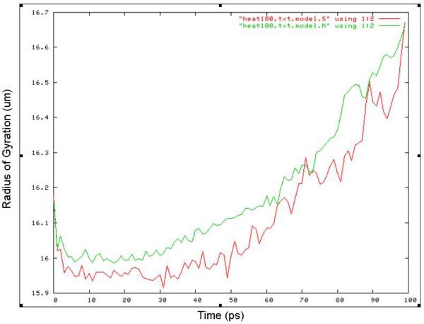
Unfolding simulations for p53 mutants were performed with linearly increasing temperature from 40K to 1,000K over 100 picoseconds. Radius of gyration in an unfolding trajectory was monitored to correlate with thermodynamic stability. Three molecular dynamics runs were performed to reduce uncertainty in the trajectories.
3.4 Features
Computational analyses used molecular model-based representations to create the component classifiers: (1D) genomic sequence, (2D) surface property maps, (3D) protein structure distance maps, and (4D) unfolding trajectories over time. Feature selection was done inside the cross-validation loop. As a control, two string-based classifiers also were constructed.
3.4.1 Sequence (1D)
Information about the location of the mutation and the residue change was used to construct the set of 1D structure features. Secondary structure information of the mutation (alpha helix, beta sandwich, etc.) was recorded with its general location in the p53 core domain (S1, S2, H1, H2). The residue property change was recorded: polarity, amino acid substitution, size, charge, aromaticity, hydrophobicity, and if in a DNA-binding region. Stability predictions from MUpro7 Error! Reference source not found. were also included, resulting in 247 features per mutant.
3.4.2 Surface property maps (2D)
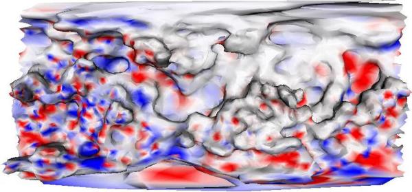
In its role as “guardian of the genome,” p53 interacts with many molecules. The 2D surface maps the p53 surface that is available for molecular interactions and drug binding (see Fig. 3).
Fig. 3.
An example of a 2D surface property map. The peaks and valleys show physical topographies on the surface of the p53. The colors indicate electrostatic charge at those positions. Red indicates a negative charge and blue indicates a positive charge.
The 2D surface property maps were annotated with surface properties, such as electrostatics or h-bond donor/acceptor status provided by the electrostatic add-ons to AMBER 6 by coauthors Lu and Luo [39]. The molecular surface was mapped to a sphere, steric and depth information was recorded and the sphere was mapped to a plane.
The resulting surface map was subtracted from the wild-type map, and a raw set of 4,883 steric surface map features and 4,895 electrostatic surface map features were extracted. A cross-validated mutual information algorithm selecting the 3,000 most relevant features (selected inside the cross-validation loop) resulted in the best classifier.
3.4.3 Protein structure distance maps (3D)
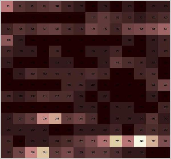
A structural mutation perturbs the molecular structure. The 3D distance map is an NxN matrix giving the Cartesian distance between N residue alpha carbons. It reflects structural shifts induced by the mutation. The wild-type distance map is subtracted, leaving a difference map.
The p53 core domain has 197 residues resulting in a 197×197 matrix that may be collapsed to a distance vector giving the magnitudes of the distance changes (Fig. 4). The resulting 197 length vector map had 3 features for each residue, the directional i, j, and k vectors. This resulted in 591 features per mutant.
Fig. 4.
A visualization of a 3D distance map. Each square represents a residue in the p53 core domain. Squares lighten as a residue moves further from its wild-type position. In this example mutations at residues 273 and 239 result in steric changes near residues 275, 281 and 240.
3.4.4 Heating Simulation (4D)
The thermodynamic stability of a p53 mutant is an important determinant of cancer. The unfolding of a molecular model in a simulated heat bath is related to thermodynamic stability. The 4D data tracks the 3D structure of the molecule over time. For each ps time step, the radius of gyration averaged across three runs produced a vector with 99 features per mutant (see Fig. 5).
Fig. 5.
A 4D unfolding trajectory showing two mutants with obviously different unfolding patterns.
3.4.5 String-based control
A Support Vector Machine (SVM) was used for the string-based classifiers because SVMs have been found to perform well on diverse biological data [45]. Two string based classifier methods were selected. One, hereafter called string-match based, used just k-mer match scores between sequences [46] and was optimized extensively and used in the composite classifier as an alternative 1D classifier. The other, hereafter called string-mismatch based, used slightly different k-mer match scores with a mismatch tolerance parameter [47]. Both were tested with k from 2−5 and the mismatch tolerance m was tested from 0−1 to see which produced the highest cross-validated accuracy on the known data set. Ultimately a kernel with k=4 was selected for the string-match based method and k=5 with m=0 was selected for the string-mismatch based method.
3.5 Machine learning
The WEKA machine learning software8 Support Vector Machine algorithm [48][49] was used for 1−4D component classifiers. The composite classifier was constructed using an in-house implementation of the Naive Bayes algorithm [50]. In this implementation, statistics for each of the 1−4D component classifiers and all combinations thereof are used to determine the probability of each classifier correctly predicting a mutant. Specifically, let A be the event that mutant m is active, c[i] be the i th component classifier trained on set t , Ci = c[i](m) be the prediction of c[i] on m , and Di = (C1 & C2... & Ci) with D0 = () . Then P(A | DN) , the Bayesian probability that m is active given the predictions of the N component classifiers, is estimated as follows (3),(4),(5),(6)9:
| (3) |
| (4) |
| (5) |
P(Ci | A) estimates the probability of an active or inactive prediction given an active mutant.
| (6) |
P(Ci | Di 1) estimates the probability that a given component classifier makes an active or inactive prediction given all previous component classifiers. Ultimately, a mutant with P(A | DN) greater than 0.5 was predicted to be active.
4 Results
This section gives results from 1) the preparatory analysis, 2) the double-blind trials, and 3) the post-mortem analysis.
4.1 Preparatory Analysis
Table 1 summarizes the composite classifier on K1, the initial training set of 123 mutants.
Table 1.
Cross-validated Composite Classifier Accuracy
| Train | Test | Accuracy | Correlation |
|---|---|---|---|
| K1 | K1 | 72.2 | 0.44 |
K1 is the initial set of known mutants cross-validated using OECV (section 2.1).
Table 2 shows each component classifier in cross-validated predictions, also on K1.
Table 2.
Cross-validated accuracy of the component classifiers
| String-match | 1D | 2D | 3D | 4D | |
|---|---|---|---|---|---|
| Accuracy | 52.0% | 74.0% | 65.0% | 73.2% | 47.2% |
Accuracies calculated using data set K1.
Table 3 quantifies the correlation between predictions produced by the component classifiers.
Table 3.
Component classifier correlations
| Set | C | String-match | 1D | 2D | 3D | 4D |
|---|---|---|---|---|---|---|
| C | 1 | 0.13 | 0.68 | 0.71 | 0.62 | −0.06 |
| String-match | 1 | 0.03 | 0.00 | 0.23 | 0.10 | |
| 1D | 1 | 0.45 | 0.61 | −0.07 | ||
| 2D | 1 | 0.51 | 0.00 | |||
| 3D | 1 | −0.13 | ||||
| 4D | 1 |
Correlation between the component classifiers (1D-4D), the string-match based control and the composite classifier (C) created using cross-validated K1.
4.2 Double-Blind Trials
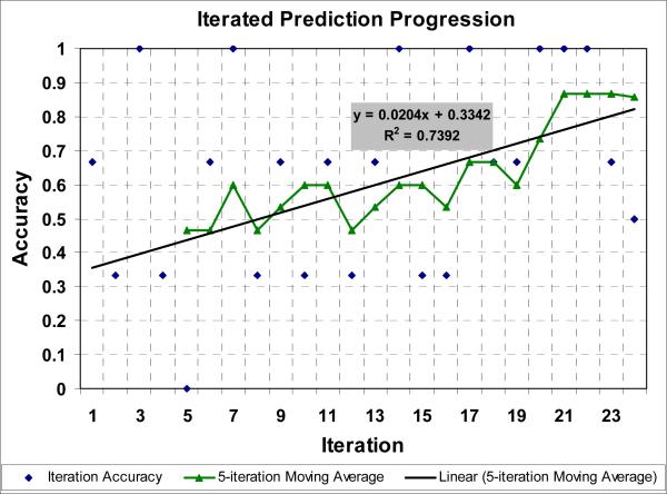
Table 4 presents the raw results achieved during the 24 iterations from section 2.1. Fig. 6 shows accuracies derived from Table 4. Accuracy is shown for both the predictions made in each iteration (predicting one group of three mutants) and for a moving window of 5-iteration moving average. As expected, prediction accuracy begins low (47% for the initial 15-point moving average) and climbs throughout the course of the experiment as the most informative mutants are identified and added to the training set (86% for the final 14-point moving average).
Fig. 6.
Prediction Accuracy. The diamonds show the prediction accuracy for each iteration. The triangle marked line shows a 5-iteration moving window with a linear regression line.
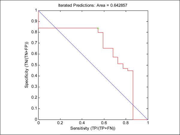
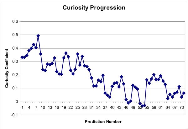
Table 5 summarizes the predictive accuracy of the classifier on the double-blind test set. Fig. 7 shows a ROC curve, and Table 6 shows a 2×2 confusion matrix, for the predictions shown in Table 4. Fig. 8 shows the curiosity outlined in section 2.1.2. As expected, the mutants selected initially were more informative than those deferred until later in the process.
Fig. 7.
A ROC curve from the composite classifier predicting X1-X24. A cutoff of 0.5 is used to determine whether active or inactive is predicted.
Table 6.
A confusion matrix for the X1-X24 predictions
| Positive | Negative | |
|---|---|---|
| True | 15 | 30 |
| False | 19 | 7 |
Fig. 8.
This figure shows the sum of curiosity values for all component classifiers (section 2.1.2) calculated for each of the three mutants chosen during each iteration of the iterated predictor.
4.3 Post-Mortem Analysis
Table 7 shows the cross-validated accuracy of the final mutant set (K25) predicting the behavior of different mutant subsets.
Table 7.
Cross-Validated Composite Classifier Accuracies
| Train | Test | Accuracy | Correlation |
|---|---|---|---|
| K25 | X1-X24 (Post) | 71.8% | 0.33 |
| K25 | K1 | 69.1% | 0.36 |
| K25 | K25 | 69.1% | 0.34 |
Variables as defined in Table 5. K25, X1-X24 (Post) is the cross-validated accuracy predicting X1-X24 using K25 where K25 = (K1 + X1-X24). All trials were cross-validated using OECV (section 2.1.3).
4.3.1 String-based Control
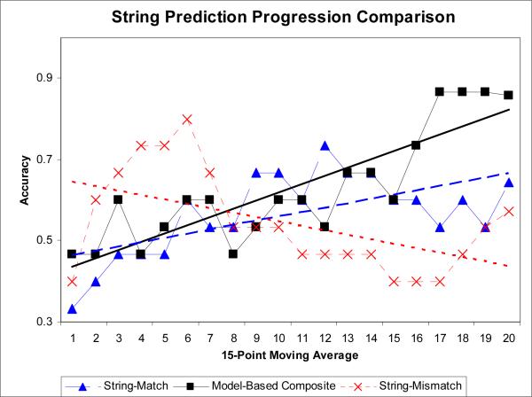
We repeated the predictions using the same training and test sets in the same order as shown in Table 5 and Fig. 6 using two string-based controls (section 3.4.5) as a direct comparison to the model-based classifiers (sections 3.4.1−3.4.4). Fig. 9 shows the composite prediction accuracy versus string-match based and string-mismatch based prediction accuracy. While predictive accuracy of the string-match based k-mer predicter did increase over time it was substantially lower than for model-based features. The string-mismatch based classifier accuracy demonstrated no clear pattern.
Table 5.
Double-Blind Composite Classifier Accuracies
| Train | Test | Accuracy | Correlation |
|---|---|---|---|
| K1 | X1-X24 (Pre) | 53.5% | −0.09 |
| K1-K5* | X1-X5* | 46.7% | 0.17 |
| K1-K24* | X1-X24* | 63.4% | 0.00 |
| K20-K24* | X20-X24* | 85.7% | 0.69 |
K1 and X1-X24 are the initial sets of known and unknown mutants (respectively). K1, X1-X24 (Pre) is a double-blind prediction using K1 to predict X1-X24. Ky-Kz*, Xy-Xz* are iterated predictions using sets Ky-Kz to predict iterations Xy-Xz (respectively).
Fig. 9.
A comparison between the composite classifier and the two string-based classifiers.
4.3.2 Random Control
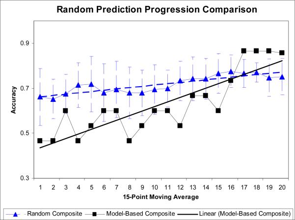
A baseline for active learning is established by control trials wherein mutants are selected randomly. Fig. 10 shows the prediction progression using active learning (section 2.1.2) versus the prediction progression using randomly selected mutants. Their accuracy increased slightly as more training data was added, but much less than the curiosity-based active learning.
Fig. 10.
A comparison between the composite classifier runs using active learning and using randomly selected mutants. The error bars show one standard deviation across 15 trials.
5 Classifier methodology improvements
As discussed in section 2.1.4, the computational models and biological experiments synergistically evolve while exploring the mutant space.
5.1 Motivation to Improve 2D Component Classifier
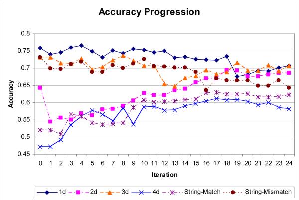
As demonstrated in section 4.2, the composite classifier accuracy improved considerably while performing the iterated predictions. When analyzed in terms of the cross-validated component classifier accuracy, two trends became apparent (see Fig. 11). The 1D classifier fell slightly in cross-validated accuracy from approximately 75.8% to 69.1% while the 2D classifier rose in cross-validated accuracy from 64.2% to 72.2%.
Fig. 11.
Cross-validated component classifier accuracy sampled during the iterated predictions. The 3D and especially the 1D accuracy fell while the 2D accuracy improved considerably.
5.1.1 Surface Evolution by Functional Region
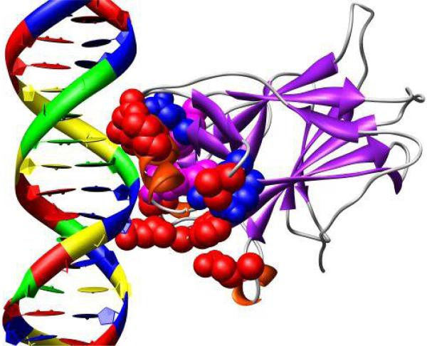
DNA and almost all small molecules bind to p53 around a promiscuous binding domain [51] on the surface of amino acids 94−160 and 264−315. The 2D surface was modified so that regions not in the promiscuous binding region were sampled at a lower resolution: each amino acid was reduced to one surface position feature and one surface electrostatic feature. Regions within the promiscuous binding domain were sampled at the resolution described in section 3.4.2. This resulted in 4,826 features rather than the 9,778 used during the iterated predictions (see section 3.4.2). Several different feature set sizes were tested using the Weka8 Mutual Information algorithm [52] and 400 features yielded the consistently highest cross-validated accuracy across several training sets. The regions selected by the Mutual Information algorithm on K25 can be represented visually as shown in Fig. 12 [53]. Most of the relevant residues cluster around the DNA binding region or around residue Y103.
Fig. 12.
Residues selected by mutual information value. Residues selected for just their electrostatic components appear in red, steric features appear in blue and both steric and electrostatic features appear in magenta. The DNA binding region is frequently selectecd and therefore inferred to be important. Some less frequently selected residues cluster around residue Y103 on the other side of the protein (data not shown).
5.1.2 New 2D Results
Table 8 shows the cross-validated accuracy for the 2D and composite classifiers using both the old and new 2D feature selection techniques.
Table 8.
Results of methodology improvements
| TP | FP | FN | TN | ACC | CC | |
|---|---|---|---|---|---|---|
| Old 2D (Component) |
40 | 24 | 34 | 96 | 70.1% | 0.35 |
| New 2D (Component) |
50 | 22 | 24 | 98 | 76.3% | 0.50 |
| Old 2D Old Composite |
43 | 29 | 31 | 91 | 69.1% | 0.34 |
| New 2D Old Composite |
47 | 29 | 27 | 91 | 71.1% | 0.39 |
| New 2D New Composite |
45 | 25 | 29 | 95 | 72.2% | 0.40 |
Cross-validated accuracy for methodological improvements predicting the 194 mutants in K25. The Old 2D feature selection outlined in Section 3.4.2 used 3000 features, while the New 2D feature selection shown here used 400 features. The New Composite is outlined in Section 5.2.
5.2 Improved Composite Classifier
As per Table 8, a significant improvement in the 2D component classifier resulted in a small improvement in the overall composite classifier. To correct this, the composite classifier outlined in Section 3.5 was modified to weight more heavily component classifiers that did particularly well. For each component classifier the score of correctly predicting an active (Q(A | Di)) or inactive (Q(I | Di)) mutant is shown in (6) and (7) respectively.
| (6) |
| (7) |
The final prediction was calculated using (11):
| (8) |
where α and β are normalization constants over all component classifiers predicting active and inactive respectively. A mutant is considered active if Q > 0 (8).
6 Discussion
This paper demonstrated a coordinated computational and experimental attack on the functional genomics of p53 cancer and suppressor mutants. To our knowledge, it is the first large-scale attempt to predict the phenotypic functional rescue of p53 cancer mutants. It showed:
A double-blind test of the functional census methodology on p53 cancer rescue mutants (see section 2.1). Predictive accuracy rose over the course of the trial (see Fig. 6) and the more informative mutants were selected early (see Fig. 8).
Machine learning and statistical predictions working in synergy with molecular modeling (see section 2.2). Model-based classifiers out-performed string-based classifiers in a control experiment (see Fig. 9). The composite classifier was relatively accurate (over 80%) when predicting cancer mutants V173L, Y205C, and R273H (see Table 4). However, it was inaccurate on cancer mutants R158L, Y220C, and G245S. We believe that more informative rescue mutants can be selected for these cancer mutants, and additional trials are in progress.
It is surprising that the 4D unfolding trajectories lagged in predictive power, since they bear information about thermostability and p53 is a thermosensitive molecule. Nonetheless, 1000K is very high and 100 ps is very short. More biologically realistic unfolding regimes may help.
By analyzing the results of each round of predictions, new information about p53 and a better way to construct the classifier became available. This information was used to improve the classifier (see section 5) and may also aid in understanding p53.
6.1 Implications
The biological advance is a general method to catalog mutation sequence spaces across important proteins of medical interest, which may eventually extend to medical knowledge of entire pathways and networks. The computational advance is a method whereby robust statistical methods applied to noisy, biased, imperfect molecular models help experimentalists to pursue function in areas where previously the techniques were believed not to apply.
The broad goal is a comprehensive census of the functional rescue of p53 cancer mutants by second-site suppressor mutations. A functional census of suppressor mutations for p53 cancer mutants will significantly further our knowledge of p53 rescue mechanisms. Knowledge of all regions of the p53 core domain that improve stability when altered will provide guidance in choosing possible docking sites for small molecules.
The methodology generalizes to other mutational systems where mutants can be classified as active or inactive. Computational classifiers that predict mutant function will allow experimentalists to map structure/function relationships for proteins in other mutation-related diseases.
6.2 Conclusion
Central to the goal of cancer treatment by p53 functional rescue is better knowledge of p53 rescue mechanisms. Intragenic suppressor mutations pinpoint key regions of the p53 core domain that may be modified to increase stability of or restore binding domains in the p53 protein. This gives a validated point of control that restores native p53 function, and identifies the cancer mutants that are amenable to functional rescue and thus the most likely drug targets. Our long-term goal is to exploit these findings for the design of drug compounds that can restore p53 function, and preliminary small molecule studies are underway with our collaborators.
ACKNOWLEDGMENTS
We thank Richard Chamberlin, Melanie Cocco, Richard Colman, John Coroneus, Hartmut Luecke, Don Senear, and Ying Wang for contributions to the larger collaborative p53 functional rescue project. Thanks to the UCI office of Research and Graduate Studies, and the UCI Institute for Genomics and Bioinformatics, for financial support. Work supported in part by NIH Biomedical Informatics Training grant (LM-07443−01), NSF MRI grant (EIA-0321390) to P.B., NIH BISTI grant (CA-112560) and NSF ITR grant (0326037) to R.H.L., NIH grant (CA81511) to R.K.B., Harvey Fellowship to S.J.S., and the UCI Medical Scientist Training Program.
Biography
Samuel A. Danziger received a B.S. in Electrical Engineering and a M.S. in Computer Science in 2002 from the Rochester Institute of Technology. He earned a M.S. in Biomedical Engineering in 2003 from the University of California, Irvine, where he is funded by the NIH Biomedical Informatics Training grant and current persuing his PhD. He is a member of IEEE and the IEEE Biomedical Engineering Society.
S. Joshua Swamidass recieved a B.S. in Biology, minoring in Computer Science, in 2000 from the University of California, Irvine (UCI). He is currently an MD/PhD student in the NIH funded Medical Scientist Training Program of the UCI College of Medicine. His PhD will be awarded by the School of Information and Computer Science.
Jue Zeng received B.S. of Biochemistry and Molecular Biology from Peking University (China) in 1996. After M.S. of Biology and Bioengineering from Syracuse University in 2001 she started working on p53-related projects in the Brachmann laboratory.
Lawrence R. Dearth received his B.A. in Biology from the University of Hawaii at Manoa in 1994. He went on to earn his Ph.D. in Molecular, Cellular and Developmental Biology from The Ohio State University in 2002. Since 2003 he is a postdoctoral fellow in the laboratory of Dr. Rainer Brachmann. Recently, Dr. Dearth was awarded a Postdoctoral Fellowship from the Susan G. Komen Foundation to pursue work on the functional inactivation of wild-type p53 in human breast cancers.
Dr. Qiang Lu received a B.S. in Physics in 1994 from Northeast University, a M.S. in Physics from Dalian Institute of Technology, and a Ph.D. in Theoretical Physics in 2000 from Nankai University. He was a Lecturer in the Department of Physics in Nankai University from 2000 to 2002. He continued his research training in biophysics at the University of California, Irvine, and the State University of New York, Stony Brook. Qiang is a member of the American Chemical Society.
Jonathan Chen received a B.S in Cybernetics with a specialization in Computer Studies in 2000 from the University of California, Los Angeles. He is currently an MD/PhD student at the University of California, Irvine pursuing a joint degree with the department of Information & Computer Science, supported by the NIH Medical Scientist Training Program. Outside of academia, he has been employed as a software developer at Trilogy Software in Austin, TX and the 20th Century Fox, Information Technology department. Current research interests focus on large-scale chemical informatics to aid tasks ranging from drug discovery to broad explorations of chemical space.
Jianlin Cheng received a B.S. in computer science from the Huazhong University of Science and Technology in China in 1994. He earned a M.S. in computer science from Utah State University in 2001. He is currently a Ph.D candidate in computer science at the Institute for Genomics and Bioinformatics in the School of Information and Computer Sciences of the University of California, Irvine. His research interests include algorithms and applications for bioinformatics, systems biology, and machine learning.
Vinh P. Hoang received a B.S. in Computer Science from the Donald Bren School of Computer Science from the University of California, Irive in 2004. Vinh is currently working as a Software Developer at Raytheon and pursuing his M.S. at the University of California, Irvine in the field of BioInformatics.
Hiroto Saigo received a B.S. in Electrical & Electronics Engineering from Sophia University in 2001, and a Master of Informatics from Kyoto University in 2003. He is currently a Ph.D candidate in Dept. of Intelligence Science and Technology in Graduate School of Informatics at Kyoto University. His research interests are in algorithms and applications in bioinformatics field, especially in machine learning methods.
Dr. Ray Luo received a B.S. in Biophysics in 1990 from Beijing University and a Ph.D. in Chemistry in 1998 from University of Maryland—College Park. He continued his research training at the University of California--San Francisco as a postdoctoral fellow before starting his own research group at the University of California--Irvine in 2001. His research is supported in part by NIH (R01 GM069620) and CRCC (35140). Ray is a member of the American Chemical Society and Biophysical Society.
Dr. Pierre Baldi received his PhD in Mathematics from the California Institute of Technology in 1986. He has held postdoctoral, faculty, and member of the technical staff positions at UCSD and Caltech, in the Division of Biology and the Jet Propulsion Laboratory. He was CEO of a startup company for a few years and joined UCI in 1999. He is now Professor in the School of Information and Computer Sciences with joint appointment in the Department of Biological Chemistry, and Director of the UCI Institute for Genomics and Bioinformatics. He received the Lew Allen Award at JPL in 1993 and the Laurel Wilkening Faculty Innovation Award at UCI. Dr. Baldi's has published four books and over 100 scientific articles. His research focuses on the application of AI and machine learning methods to problems in the life-sciences. His main contributions have been in the area of statistical machine learning and bioinformatics, including the development of Hidden Markov Models (HMMPro) for sequence analysis, recursive neural networks for de novo protein structure prediction (SCRATCH), Bayesian statistical methods for DNA microarray analysis (Cyber-T), and more recently kernel methods in chemical informatics. The work of his group has resulted in several databases, software, and web servers that are widely used (www.igb.uci.edu/servers/servers.html).
Dr. Rainer K. Brachmann obtained his M.D. from the Ludwig-Maximilians-University in Munich, Germany, and is a medical oncologist. His laboratory studies the pathway of the tumor suppressor protein p53 with particular emphasis on the novel therapeutic strategy of restoring function to p53 cancer mutants. He is a member of the AACR.
Dr. Richard H. Lathrop received a B.A. in Mathematics from Reed College (1978), and a master's in Computer Science (1983), the graduate degree of Electrical Engineer (1983), and a Ph.D. in Artificial Intelligence (1990) from the Massachusetts Institute of Technology. He is a Professor in the Bren School of Information and Computer Sciences at the University of California, Irvine. He is on the Editorial Boards of Molecular and Cellular Proteomics (2001--present) and IEEE Intelligent Systems (2002--present). He received Best Paper Awards from the International Conference on Genome Informatics (2001), the ACM/IEEE International Design Automation Conference (1987) and an Innovative Application Award from the AAAI/IAAI Conference (1998). He has over 65 scientific and technical publications, and his research has appeared on the cover of AI Magazine (1999), Journal of Molecular Biology (1996), and Communications of the ACM (1987). He was a co-founding scientist of Arris Pharmaceutical Corp. and of CODA Genomics, Inc., served on the Scientific Advisory Boards of CombiChem, Inc., and GeneFormatics, Inc., and was a founding Officer (Treasurer) and member of the founding Board of Directors of the International Society for Computational Biology (1996). His research interests are in artificial intelligence and computational biology. He is a member of IEEE (Computer Society), AAAI (Life Member), ACM, and ISCB.
Footnotes
This abuse of notation, + as set union instead of U, was found to be more intuitive to a wider audience.
PDB ID: 1tsr. Chain B
frcmod.mod_phipsi.2 in the AMBER 8 distribution
Contributor Information
Samuel A. Danziger, University of California, Irvine, CA 92697. E-mail: Sam_Danziger@ieee.org
S. Joshua Swamidass, University of California, Irvine, CA 92697. E-mail: sswamida@uci.edu.
Jue Zeng, University of California, Irvine, CA 92697. E-mail: jzeng@uci.edu.
Lawrence R. Dearth, University of California, Irvine, CA 92697. E-mail: ldearth@uci.edu
Qiang Lu, State University of New York, Stony Brook, NY 11794. E-mail: Qiang.Lu@stonybrook.edu.
Jonathan H. Chen, University of California, Irvine, CA 92697. E-mail: chenjh@uci.edu
Jainlin Cheng, University of California, Irvine, CA 92697. E-mail: jianlinc@ics.uci.edu.
Vinh P. Hoang, University of California, Irvine, CA 92697. E-mail: vphoang@uci.edu
Hiroto Saigo, University of California, Irvine, CA 92697. E-mail: hiroto@kuicr.kyoto-u.ac.jp.
Ray Luo, University of California, Irvine, CA 92697. E-mail: rluo@uci.edu.
Pierre Baldi, University of California, Irvine, CA 92697 E-mail: pfbaldi@uci.edu.
Rainer K. Brachmann, University of California, Irvine, CA 92697 E-mail: rbrachma@uci.edu
Richard H. Lathrop, University of California, Irvine, CA 92697 E-mail: rickl@uci.edu
References
- 1.Rubin DL, Shafa F, Oliver DE, Hewett M, Altman RB. Representing genetic sequence data for pharmacogenomics: an evolutionary approach using ontological and relational models. Bioinformatics. 2002;18(Suppl 1):S207–215. doi: 10.1093/bioinformatics/18.suppl_1.s207. [DOI] [PubMed] [Google Scholar]
- 2.Lathrop RH, Pazzani MJ. Combinatorial optimization in rapidly mutating drug-resistant viruses. J Combinatorial Optimization. 1999;3:301–320. [Google Scholar]
- 3.Lathrop RH, Steffen NR, Raphael M, Deeds-Rubin S, Pazzani MJ, Cimoch PJ, See DM, Tilles JG. Knowledge-based avoidance of drug-resistant HIV mutants. AI Magazine. 1999;20:13–25. [Google Scholar]
- 4.Beerenwinkel N, Lengauer T, Selbig J, Schmidt B, Walter H, Korn K, Kaiser R, Hoffman D. Geno2pheno: interpreting genotypic HIV drug resistance tests. IEEE Intelligent Systems. 2001;16:35–41. [Google Scholar]
- 5.Bush MR, Bender CA, Subbarao KC, Nancy J, Fitch WM. Predicting the Evolution of Human Influenza A. Science. 1999;286:1921–1925. doi: 10.1126/science.286.5446.1921. [DOI] [PubMed] [Google Scholar]
- 6.Wahl GM, Carr AM. The evolution of diverse biological responses to DNA damage: insights from yeast and p53. Nat Cell Biol. 2001;3:E277–286. doi: 10.1038/ncb1201-e277. [DOI] [PubMed] [Google Scholar]
- 7.Xu Y. Regulation of p53 responses by post-translational modifications. Cell Death Differ. 2003;10:400–403. doi: 10.1038/sj.cdd.4401182. [DOI] [PubMed] [Google Scholar]
- 8.Appella E, Anderson CW. Post-translational modifications and activation of p53 by genotoxic stresses. Eur J Biochem. 2001;268:2764–2772. doi: 10.1046/j.1432-1327.2001.02225.x. [DOI] [PubMed] [Google Scholar]
- 9.Brooks CL, Gu W. Ubiquitination, phosphorylation and acetylation: the molecular basis for p53 regulation. Curr Opin Cell Biol. 2003;15:164–171. doi: 10.1016/s0955-0674(03)00003-6. [DOI] [PubMed] [Google Scholar]
- 10.el-Deiry WS, Kern SE, Pietenpol JA, Kinzler KW, Vogelstein B. Definition of a consensus binding site for p53. Nat Genet. 1992;1:45–49. doi: 10.1038/ng0492-45. [DOI] [PubMed] [Google Scholar]
- 11.Funk WD, Pak DT, Karas RH, Wright WE, Shay JW. A transcriptionally active DNA-binding site for human p53 protein complexes. Mol Cell Biol. 1992;12:2866–2871. doi: 10.1128/mcb.12.6.2866. [DOI] [PMC free article] [PubMed] [Google Scholar]
- 12.Qian H, Wang T, Naumovski L, Lopez CD, Brachmann RK. Groups of p53 target genes involved in specific p53 downstream effects cluster into different classes of DNA binding sites. Oncogene. 2002;21:7901–7911. doi: 10.1038/sj.onc.1205974. [DOI] [PubMed] [Google Scholar]
- 13.Kannan K, Amariglio N, Rechavi G, Jakob-Hirsch J, Kela I, Kaminski N, Getz G, Domany E, Givol D. DNA microarrays identification of primary and secondary target genes regulated by p53. Oncogene. 2001;20:2225–2234. doi: 10.1038/sj.onc.1204319. [DOI] [PubMed] [Google Scholar]
- 14.Polyak K, Xia Y, Zweier JL, Kinzler KW, Vogelstein B. A model for p53-induced apoptosis. Nature. 1997;389:300–305. doi: 10.1038/38525. [DOI] [PubMed] [Google Scholar]
- 15.Caelles C, Helmberg A, Karin M. p53-dependent apoptosis in the absence of transcriptional activation of p53-target genes. Nature. 1994;370:220–223. doi: 10.1038/370220a0. [DOI] [PubMed] [Google Scholar]
- 16.Manfredi JJ. p53 and apoptosis: it's not just in the nucleus anymore. Mol Cell. 2003;11:552–554. doi: 10.1016/s1097-2765(03)00106-0. [DOI] [PubMed] [Google Scholar]
- 17.Mihara M, Erster S, Zaika A, Petrenko O, Chittenden T, Pancoska P, Moll UM. p53 has a direct apoptogenic role at the mitochondria. Mol Cell. 2003;11:577–590. doi: 10.1016/s1097-2765(03)00050-9. [DOI] [PubMed] [Google Scholar]
- 18.Olivier M, Eeles R, Hollstein M, Khan MA, Harris CC, Hainaut P. The IARC TP53 Database: new online mutation analysis and recommendations to users. Hum Mutat. 2002 Jun;19(6):607–14. doi: 10.1002/humu.10081. [DOI] [PubMed] [Google Scholar]
- 19.Beroud C, Soussi T. The UMD-p53 database: new mutations and analysis tools. Hum Mutat. 2003;21:176–181. doi: 10.1002/humu.10187. [DOI] [PubMed] [Google Scholar]
- 20.Cho Y, Gorina S, Jeffrey PD, Pavletich NP. Crystal structure of a p53 tumor suppressor-DNA complex: understanding tumorigenic mutations. Science. 1994;265:346. doi: 10.1126/science.8023157. [DOI] [PubMed] [Google Scholar]
- 21.Bullock AN, Henckel J, DeDecker BS, Johnson CM, Nikolova PV, Proctor MR, Lane DP, Fersht AR. Thermodynamic stability of wild-type and mutant p53 core domain. Proc Natl Acad Sci U S A. 1997;94:14338–14342. doi: 10.1073/pnas.94.26.14338. [DOI] [PMC free article] [PubMed] [Google Scholar]
- 22.Bullock AN, Henckel J, Fersht AR. Quantitative analysis of residual folding and DNA binding in mutant p53 core domain: definition of mutant states for rescue in cancer therapy. Oncogene. 2000;19:1245–1256. doi: 10.1038/sj.onc.1203434. [DOI] [PubMed] [Google Scholar]
- 23.Wong KB, DeDecker BS, Freund SM, Proctor MR, Bycroft M, Fersht AR. Hot-spot mutants of p53 core domain evince characteristic local structural changes. Proc Natl Acad Sci U S A. 1999;96:8438–8442. doi: 10.1073/pnas.96.15.8438. [DOI] [PMC free article] [PubMed] [Google Scholar]
- 24.Levine AJ. p53, the cellular gatekeeper for growth and division. Cell. 1997;88:323–331. doi: 10.1016/s0092-8674(00)81871-1. [DOI] [PubMed] [Google Scholar]
- 25.Prives C, Hall PA. The p53 pathway. J Pathol. 1999;187:112–126. doi: 10.1002/(SICI)1096-9896(199901)187:1<112::AID-PATH250>3.0.CO;2-3. [DOI] [PubMed] [Google Scholar]
- 26.Vogelstein B, Lane D, Levine AJ. Surfing the p53 network. Nature. 2000;408:307–310. doi: 10.1038/35042675. [DOI] [PubMed] [Google Scholar]
- 27.Vousden KH. p53: death star. Cel. 2000;103:691–694. doi: 10.1016/s0092-8674(00)00171-9. [DOI] [PubMed] [Google Scholar]
- 28.May P, May E. Twenty years of p53 research: structural and functional aspects of the p53 protein. Oncogene. 1999;18:7621–7636. doi: 10.1038/sj.onc.1203285. [DOI] [PubMed] [Google Scholar]
- 29.Foster BA, Coffey HA, Morin MJ, Rastinejad F. Pharmacological rescue of mutant p53 conformation and function. Science. 1999;286:2507–2510. doi: 10.1126/science.286.5449.2507. [DOI] [PubMed] [Google Scholar]
- 30.Bykov VJN, Issaeva N, Shilov A, Hultcrantz M, Pugacheva E, Chumakov P, Bergman J, Wiman KG, Selivanova G. Restoration of the tumor suppressor function to mutant p53 by a low-molecular-weight compound. Nat Med. 2002;8:282–288. doi: 10.1038/nm0302-282. [DOI] [PubMed] [Google Scholar]
- 31.Brachmann RK, Yu K, Eby Y, Pavletich NP, Boeke JD. Genetic selection of intragenic suppressor mutations that reverse the effect of common p53 cancer mutations. EMBO J. 1998;17:1847–1859. doi: 10.1093/emboj/17.7.1847. [DOI] [PMC free article] [PubMed] [Google Scholar]
- 32.Baroni TE, Wang T, Qian H, Dearth L, Troung LN, Zeng J, Denes AE, Chen SW, Brachmann RK. A global suppressor motif for p53 cancer mutants. PNAS. 2004;101 14:4930–4935. doi: 10.1073/pnas.0401162101. [DOI] [PMC free article] [PubMed] [Google Scholar]
- 33.Bullock AN, Fersht AR. Rescuing the Function of Mutant p53. Nat Rev Cancer. 2001;1(1):68–76. doi: 10.1038/35094077. [DOI] [PubMed] [Google Scholar]
- 34.Martin AC, Facchiano AM, Cuff AL, Hernandez-Boussard T, Olivier M, Hainaut P, Thornton JM. Integrating mutation data and structural analysis of the TP53 tumor-suppressor protein. Hum Mutat. 2002;19:149–164. doi: 10.1002/humu.10032. [DOI] [PubMed] [Google Scholar]
- 35.Warmuth MK, Liao J, Raetsch G, Mathieson M, Putta S, Lemmen C. Active Learning with Support Vector Machines in the Drug Discovery Process. J Chem. inf. Comput. Sci. 2003;43:667–673. doi: 10.1021/ci025620t. [DOI] [PubMed] [Google Scholar]
- 36.Liu Y. Active Learning with Support Vector Machine Applied to Gene Expression Data for Cancer Classification. J Chem. Inf. Comput. Sci. 2004;44:1936–1941. doi: 10.1021/ci049810a. [DOI] [PubMed] [Google Scholar]
- 37.Mitra P, Murthy CA, Pal SK. A Probabilistic Active Support Vector Learning Algorithm. IEEE Transactions on Pattern Analysis and Machine Intelligence. 2004;26:413–418. doi: 10.1109/TPAMI.2004.1262340. [DOI] [PubMed] [Google Scholar]
- 38.Karchin R, Diekhans M, Kelly L, Thomas DJ, Pieper U, Eswar N, Haussler D, Sali A. LS-SNP: large-scale annotation of coding non-synonymous SNPs based on multiple information sources. Bioinformatics. 2005;21:2814–2820. doi: 10.1093/bioinformatics/bti442. [DOI] [PubMed] [Google Scholar]
- 39.Case DA, Darden TA, Cheatham TE, III, Simmerling CL, Wang J, Duke RE, Luo R, Merz KM, Wang B, Pearlman DA, Crowley M, Brozell S, Tsui V, Gohlke H, Mongan J, Hornak V, Cui G, Beroza P, Schafmeister C, Caldwell JW, Ross WS, Kollman PA. AMBER 8. University of California; San Francisco: 2004. [Google Scholar]
- 40.Tsui V, Case DA. Theory and applications of the generalized Born solvation model in macromolecular simulations. Biopolymers (Nucl. Acid. Sci. 2001;56:275–291. doi: 10.1002/1097-0282(2000)56:4<275::AID-BIP10024>3.0.CO;2-E. [DOI] [PubMed] [Google Scholar]
- 41.Ryckaert J-P, Ciccotti G, Berendsen HJC. Numerical integration of the cartesian equations of motion of a system with constraints: Molecular dynamics of n-alkanes. J. Comput. Phys. 1977;23:327–341. [Google Scholar]
- 42.Canutescu AA, Shelenkov AA, Dunbrack RL., Jr. A graph theory algorithm for protein side-chain prediction. Protein Science. 2003;12:2001–2014. doi: 10.1110/ps.03154503. [DOI] [PMC free article] [PubMed] [Google Scholar]
- 43.Press WH, Teukolsky SA, Vetterling WT, Flannery BP. Numerical Recipes, The Art of Scientific Computing. 2nd Edition Cambridge University Press; Cambridge: 1992. [Google Scholar]
- 44.Cheng J, Randall A, Baldi P. Prediction of Protein Stability Changes for Single Site Mutations Using Support Vector Machines. Proteins: Structure, Function, Bioinformatics. 2005 doi: 10.1002/prot.20810. In press. [DOI] [PubMed] [Google Scholar]
- 45.Schlkopf B, Tsuda K, Vert J. Kernel Methods in Computational Biology (Computational Molecular Biology) Bradford Books. 2004 ISBN: 0262195097. [Google Scholar]
- 46.Saigo H, Vert J, Ueda N, Akutsu T. Protein homology detection using string alignment kernels. Bioinformatics. 2004;20(11):1682–1689. doi: 10.1093/bioinformatics/bth141. [DOI] [PubMed] [Google Scholar]
- 47.Leslie CS, Eskin E, Cohen A, Weston J, Noble WS. Mismatch string kernels for discriminative protein classification. Bioinformatics. 2004;20(4):467–476. doi: 10.1093/bioinformatics/btg431. [DOI] [PubMed] [Google Scholar]
- 48.Witten IH, Frank E. Data Mining: Practical machine learning tools and techniques. 2nd Edition Morgan Kaufmann; San Francisco: 2005. [Google Scholar]
- 49.Platt J. Fast Training of Support Vector Machines using Sequential Minimal Optimization. In: Schoelkopf B, Burges C, Smola A, editors. Advances in Kernel Methods - Support Vector Learning. MIT Press; [Google Scholar]
- 50.Baldi P P, Brunak S. Bioinformatics: the machine learning approach. edn second MIT Press; Cambridge, MA: 2001. [Google Scholar]
- 51.Friedler DB, Veprintsev T, Rutherford KI, Fersht A. Binding of RAD51 and Other Peptide Sequences to a Promiscuous, Highly Electrostatic, Binding Site in p53. The Journal of Biological Chemistry. 2004 December; doi: 10.1074/jbc.M411176200. Paper in Press. [DOI] [PubMed] [Google Scholar]
- 52.Weisstein Eric W., et al. Mutual Information. MathWorld--A Wolfram Web Resource. http://mathworld.wolfram.com/MutualInformation.htm.
- 53.Sanner MF, Olson AJ, Spehner JC. Reduced surface: an efficient way to compute molecular surfaces. Biopolymers. 1996;38(3):305–320. doi: 10.1002/(SICI)1097-0282(199603)38:3%3C305::AID-BIP4%3E3.0.CO;2-Y. [DOI] [PubMed] [Google Scholar]


