Abstract
We describe a reverse integration approach for the exploration of low-dimensional effective potential landscapes. Coarse reverse integration initialized on a ring of coarse states enables efficient navigation on the landscape terrain: Escape from local effective potential wells, detection of saddle points, and identification of significant transition paths between wells. We consider several distinct ring evolution modes: Backward stepping in time, solution arc length, and effective potential. The performance of these approaches is illustrated for a deterministic problem where the energy landscape is known explicitly. Reverse ring integration is then applied to noisy problems where the ring integration routine serves as an outer wrapper around a forward-in-time inner simulator. Two versions of such inner simulators are considered: A Gillespie-type stochastic simulator and a molecular dynamics simulator. In these “equation-free” computational illustrations, estimation techniques are applied to the results of short bursts of inner simulation to obtain the unavailable (in closed-form) quantities (local drift and diffusion coefficient estimates) required for reverse ring integration; this naturally leads to approximations of the effective landscape.
INTRODUCTION
When an energy landscape perspective is applicable, the dynamics of a complex system appear dominated by gradient-driven descent into energy wells, occasional trapping in deep minima, and transitions between minima via passage over saddle points through thermal “kicks.” A paradigm for this landscape picture is the trapping of protein configurations in metastable states en route to the dominant folded state. The underlying energy landscape is often likened to a roughened funnel with trapped states corresponding to local free energy minima.1
Important features on energy surfaces include local minima and their associated basins of attraction, saddle points, and minimum energy paths (MEPs) between neighboring minima passing through these saddles. Besides the identification of such landscape features, establishing the details of their connectivity is a task of considerable importance. Knowledge of the relative depths of landscape minima provides thermodynamic information. The kinetics of transitions between such states is determined by the type of terrain (smooth, rugged, etc.) that surrounds and separates them, in particular, by the location and height of the low-lying saddles. The identification of important low energy molecular conformations in computational chemistry2 and the determination of protein and peptide folding pathways,3 to name but a few, rely on an ability to perform intelligent, targeted searches of the energy landscape.
Molecular dynamics (MD) and Monte Carlo (MC) simulations on energy landscapes are typically limited in the time scales they can explore by the difference between the system thermal energy and the height of transitional energy barriers. A significant fraction of MD and MC simulation time is spent bouncing around in local minima. Energy barriers separating minima cause this type of trapping and the result is long waiting times between infrequent, but interesting, transition events. An array of techniques have been proposed to overcome such time scale limitations including bias-potential approaches,4, 5 accelerated dynamics,6 coarse-variable dynamics,7, 8 and transition path sampling,9, 10 allowing extensive exploration of the energy surface and its transition states. The adaptive bias force method11, 12 efficiently samples configurational space in the presence of high free energy barriers via estimation of the force exerted on the system along a well-defined reaction coordinate. Short bursts of appropriately initialized simulations are used in coarse-variable dynamics8 to infer the deterministic and stochastic components of motion parametrized by an appropriate set of coarse variables. The use of a history-dependent bias potential in Ref. 13 ensures that minima are not revisited, allowing for efficient exploration of a free energy surface parametrized by a few coarse coordinates. Accelerated dynamics methods such as hyperdynamics and parallel replica dynamics6 “stimulate” system trajectories trapped in local minima to find appropriate escape paths while preserving the relative escape probabilities to different states. Transition path sampling9 generalizes importance sampling to trajectory space and requires no prior knowledge of a suitable reaction coordinate (see also transition interface sampling14).
Many energy landscape search methods have been devised (too numerous to discuss in detail here). Single-ended search approaches (where only the initial state is known) are based on eigenvector following (mode following)2, 15, 16, 17, 18, 19 and have been used to refine details of MEPs close to saddle points;20, 21 methods purely for efficient saddle point identification also exist.22, 23, 24Chain-of-state methods are a more recent class of double-ended searches that evolve a chain of replicas (system states or images), distributed between initial and final states, in a concerted manner.25 The original elastic band method26, 27 has been refined and extended many times.28, 29 More recently string methods,30, 31, 32 which evolve smooth curves with intrinsic parametrization, have been used to locate significant paths between two states. The global terrain approach of Lucia et al.33, 34 exploits the inherent connectedness of stationary points along valleys and ridges on the landscape for their systematic identification.
We build here on the equation-free formalism of Ref. 35 whose purpose is to enable the performance of macroscopic tasks using appropriately designed computational experiments with microscopic models. The approach focuses on systems for which the coarse-grained, effective evolution equations are assumed to exist but are not available in closed form. One example is the case of legacy or black-box codes: Dynamic simulators which, given initial conditions, integrate forward in time over an interval Δt. Alternatively, the effective evolution equation for the system may be the unknown closure of a microscopic simulation model such as kinetic MC or MD. Rico-Martinez et al.36 used reverse integration in conjunction with microscopic forward-in-time simulators to access reverse time behavior of coarse variables (see also Ref. 37). Hummer and Kevrekidis8 used coarse reverse integration to trace a one-dimensional (1D) effective free energy surface (and to escape from its minima) for alanine dipeptide in water. In this paper we use reverse integration in two dimensions: A ring of system initial states is evolved (forward in time in the inner simulation and then reverse in the outer, coarse integration) to explore two-dimensional (2D) potential energy (and, ultimately, free energy) surfaces. The ring is evolved along the component of the local energy gradient (projected normal to the ring) while a nodal redistribution scheme is used that slides nodes along the ring so that they remain equidistributed in ring arc length, ensuring efficient sampling. Transformation of the independent variable in our basic ring evolution equation results in several distinct stepping modes. The work in this paper follows 2D surfaces that can be “swept by” a ring. We mention the work of Henderson38, 39 for computational exploration of higher-dimensional manifolds (up to dimension 6 has been reported). The computational effort scales exponentially with the manifold dimension (the number of coarse variables in our case).
The paper is organized as follows. In Sec. 2 we present our reverse ring integration approach. Ring evolution equations are developed with time, arc length, or (effective) potential energy as the independent variable. We illustrate these stepping modes for a deterministic problem with a smooth energy landscape (Müller–Brown potential). In Sec. 3 reverse ring integration is investigated for two “noisy” problems: A Gillespie-type stochastic simulation and a MD simulation of a protein fragment in water. Estimates of the numerical values of the quantities in the ring evolution equation are found by data processing of the results of appropriately initialized short bursts of the black-box inner simulator. The extension to stepping in free energy is discussed. We conclude with a brief discussion of the results and of the potential extension of the approach to more than two coarse dimensions.
REVERSE INTEGRATION ON ENERGY SURFACES
Here we present an algorithm for (low-dimensional) landscape exploration motivated by reverse projective integration, on the one hand, and by algorithms for the computation of (low-dimensional) stable manifolds of dynamical systems on the other. Reverse projective integration37 uses short bursts of forward-in-time simulation of a dynamical system to estimate a local time derivative of the system variables, which is then used to take a large reverse projective time step via polynomial extrapolation. This type of computation is intended for problems with a large separation between many fast stable modes and a few (stable or unstable) slow ones; the long-term dynamics of the problem will then lie on an attracting, invariant slow (sub)manifold. Reverse projective integration allows us to compute “in the past,” approximating solutions on this slow manifold by only using the forward-in-time simulation code.
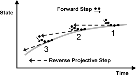
After each reverse projective step the reverse solution will be slightly off manifold (see Fig. 1); the initial part of the next short forward burst will then bring the solution back close to the manifold, while the latter part of the burst will provide the time derivative estimate necessary for the next backward step. One clearly does not integrate the full system backward in time (the fast stable modes make this problem very ill conditioned); it is the slow, on manifold backward dynamics that we attempt to follow. The approach can be used for deterministic dynamical systems of the type described; however, it was developed having in mind problems arising in atomistic∕stochastic simulation where the dynamic simulator is a MD or kinetic MC code. When (and if) the dynamics can be well described by an effective (low-dimensional) ordinary differential equation (ODE), or an effective stochastic differential equation (SDE), characterized by a potential [and by an effective (low-dimensional) free energy surface], reverse projective integration can be implemented as an outer algorithm, wrapped around the high-dimensional inner deterministic∕stochastic simulator. The combination of short bursts of fine scale inner forward-in-time simulation with data processing and estimation and then with coarse-grained outer reverse integration can then be used to systematically explore these effective potentials (and associated effective free energy surfaces).
Figure 1.
Schematic of reverse projective integration. The thick gray line indicates the position on the slow manifold as a function of time on a forward trajectory. The solid circles are configurations along microscopic trajectories run forward in time, as indicated by the short solid arrows. The long dashed arrows indicate the reverse projective steps, which result in an initialization near, but slightly off, the slow manifold.
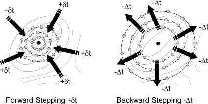
A natural set of protocols for such an exploration has already been developed (in the deterministic case) in dynamical systems theory—indeed, algorithms for the computation of low-dimensional stable manifolds of vector fields provide the “wrappers” in our context (see the review in Ref. 40). This is easily seen in the context of a 2D gradient dynamical system: An isolated local minimum of the associated potential is a stable fixed point and, locally, the entire plane is its stable manifold; the potential is a function of the points on this plane. In our 2D case, we approximate this stable manifold in the neighborhood of the fixed point by a linearization—this could be in the form of a ring of points surrounding the fixed point. One can then integrate the gradient vector field forward or backward in time (see Fig. 2) keeping track of the evolution of this initial ring; using the gradient nature of the system, one can compute, as a by-product, the potential profile.
Figure 2.
Schematic of forward and backward stepping of ring nodes (light circles) in time on an energy landscape in the vicinity of fixed point (dark circles). Solid lines are energy contours, dashed lines connect ring nodes at each step, and arrows indicate the direction of the ring evolution.
Various versions of such reverse ring integration have been previously used for visualizing 2D stable manifolds of vector fields. Johnson et al.41 evolved a ring stepping in space-time arc length (see below) with empirical mesh adaptation and occasional addition of nodes to preserve ring resolution, building up a picture of the manifold as the ring expands. Guckenheimer and Worfolk42 used algorithms based upon geodesic curve construction to evolve a circle of points according to the underlying vector field. A survey of methods for the computation of (un)stable manifolds of vector fields can be found in Ref. 40, including approaches for the approximation of k-dimensional manifolds. In this paper we will restrict ourselves to the 2D case (and thus, eventually, explore 2D effective free energy surfaces).
Clearly, forward integration of our ring constructed based on local linearization around an isolated minimum will generate a sequence of shrinking rings converging to the minimum (stable fixed point). For a 2D gradient vector field, backward (reverse) ring integration will grow the ring—and as it grows on the plane, the potential on the ring evolves uphill in the initial well, possibly toward unstable (saddle-type) stationary points.
A critical issue in tracking the reverse evolution of such a ring is its distortion, as different portions of it evolve with different rates along the stable manifold (here, the plane). Dealing with the distortion of this closed curve and the deformation of an initially equidistributed mesh of discretization points on it requires careful consideration; similar problems arise and are elegantly dealt with, in (forward-in-time) computations with the string method.30, 43 While we will first implement our reverse ring integration on a deterministic gradient problem (for descriptive clarity), our aim is to use it as a wrapper around atomistic∕stochastic inner forward-in-time simulators; two such illustrations will follow.
The deterministic two-dimensional case
Consider a simple, 2D gradient system of the form
| (2.1) |
In this case, since the vector field is explicitly available, with x in R2, we can perform reverse integration by simply reversing the sign of the right-hand side of Eq. 2.1; reverse projective integration will only become necessary in cases where the (effective) potential is not known, and the corresponding gradients need to be estimated from forward runs of a many-degree-of-freedom atomistic∕stochastic simulator. Note also that here the dependent variables x and y are known (as are the corresponding evolution equations). For high-dimensional problems with a low-dimensional effective description, selection of such good reduced variables (observables) is nontrivial; we will briefly return to this in Sec. 4.
We start with a simple illustrative example: The Müller–Brown potential energy surface,44 which is often used to evaluate landscape search methods since the MEP between its minima deviates significantly from the chord between them. We focus here on reverse ring evolution starting around a local minimum in the landscape and approaching the closest saddle point as the ring samples the well.
The potential is given by
| (2.2) |
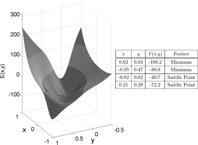
where A=(−200,−100,−170,15), a=(−1,−1,−6.5,0.7), b=(0,0,11,0.6), c=(−10,−10,−6.5,0.7), x0=(1,0,−0.5,−1), and y0=(0,0.5,1.5,1). The neighborhood of the Müller–Brown potential we explore is shown in Fig. 3 along with a listing of the fixed points, their energy, and their classification. We first discuss the initialization of the ring and then three different forms of “backward stepping:” Time stepping, arc length stepping in (phase space)×time and potential stepping. Our initial ring will be the V=−105 energy contour surrounding the minimum at (0.62,0.03).
Figure 3.
Contour map of the Müller–Brown potential for −1<x<1 and −0.5<y<1. Contour lines are shown in black (white) for V(x,y)<0 [V(x,y)>0]. Stationary points of the potential, their classification, and energy are tabulated for the region illustrated.
A ring is a smooth curve Φ, here in two dimensions. In our implementation, we discretize this curve and denote the instantaneous position of the discretized ring by the vectors Φi≡Φ(αi,t)=[x(αi,t),y(αi,t)] (with Φi in R2, αi in R) for the coordinates of the ith discretization node, where αi is a suitable parametrization. A natural choice is the normalized arc length along the ring with αi∊[0,1], as in the string method but now with periodic boundary conditions. Note that one does not need to initialize on an exact isopotential contour; keeping the analogy with local stable manifolds of a dynamical system fixed point, one can use the local linearization—and more generally, local Taylor series—to approximate a closed curve on the manifold. Anticipating the energy-stepping reverse evolution mode, however, we start with an isopotential contour here. This requires an initial point on the surface; we then trace the isopotential contour passing through this point using a scheme which resembles the sliding stage in the step and slide method of Miron and Fichthorn23 for saddle point identification. We simply “slide” along the contour to generate a curve Γ, moving (in some pseudotime τ) perpendicular to the local energy gradient according to
| (2.3) |
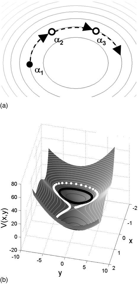
Points along the curve Γ provide initial conditions for ring nodes. Figure 4a illustrates ring initialization starting in the well, close to the isolated local minimum, resulting in a closed ring.
Figure 4.
Distribution of nodes produced by integration of Eq. 2.3 with initial condition above (white nodes and contour lines) and below (black nodes and contour lines) the saddle point energy. Below the saddle point there is a separation of isopotential contours in each well—the saddle point isopotential contours split into two.
We note that our approach is closely related to established landscape search techniques based on following Hessian eigenvectors;2, 15, 16, 17, 18, 19 here the computation is performed in a dynamical system setting: We use a dynamic simulator to estimate time derivatives (and through them local potential gradients) on demand.
Modes of reverse ring evolution
Time stepping
When every point on a curve evolves backward in time, it makes sense to consider the evolution of the entire curve in the direction of the component of the energy gradient normal to it [as also happens for forward time evolution in string methods, commonly used to identify MEPs (Ref. 30)]. Ring nodal evolution is given by
| (2.4) |
where is the unit tangent vector to Φ at Φi, with evaluated at Φi, and r is a Lagrange multiplier field30 (determined by the choice of ring parametrization) used to distribute nodes evenly along the ring. The component of the potential gradient normal to the ring (∇V)⊥ is defined as follows:
| (2.5) |
where (∇V)∥ is the component of the gradient parallel to the ring. For the general case where (∇V(Φi))⊥ is unavailable in closed form (e.g., the inner integrator is a black-box time stepper) we use (multiple short replica) simulations for each discretization node on the ring to estimate it, as will be discussed in Sec. 3. In practice, the tasks of node stepping and redistribution are often split into separate stages. The term involving r in Eq. 2.4 is first omitted, and nodal stepping is performed solving, backward in time, the N-node spatially discretized form
| (2.6) |
where Φi denotes the position of node i in the discretized ring. The normalized arc-length coordinate αi associated with the ith node is approximated using the linear distance formula
| (2.7) |
where are the coordinates of node i. Periodicity of the ring (which has N−2 distinct nodes) is imposed by the set of algebraic equations
| (2.8) |
where evaluation at time t is indicated by the subscript outside the parentheses. An explicit, backward in time, Euler discretization for the N−2 distinct nodes reads
| (2.9) |
Backward stepping in time is followed by a redistribution step that slides nodes along the ring so that they are equally spaced (or, generally, spaced in a desirable manner) in the normalized ring arc length coordinate. These two basic steps are also present in the (phase space)×time arc length or potential stepping of the ring discussed below; they are schematically summarized in Fig. 5.
Figure 5.
Stages of ring evolution: Backward stepping (in time Δt, arc length Δs, or potential ΔV) followed by nodal redistribution.
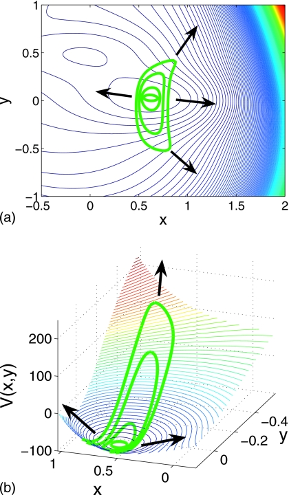
Figure 6 shows snapshots of the ring as it evolves backward in time—in the time-stepping mode—on the Müller–Brown potential. The ring quickly deviates from isopotential contours as it climbs up the well. The local speed is proportional to the local component of the potential gradient normal to the ring; wide variation in nodal speeds causes the ring to evolve unevenly, elongating along the directions of steepest ascent. Initially equispaced ring nodes would, if not redistributed, rapidly converge toward regions of high potential gradients in our parametrization, resulting in poor resolution in other areas. Even the redistribution of nodes, however, will not suffice to accurately capture the ring shape as the ring perimeter quickly grows, unless new nodes are added.
Figure 6.
Reverse time stepping on Müller–Brown potential with Δt=5×10⁻⁵ and N=80 (successive rings are shown at intervals of ten steps and arrows indicate direction of ring evolution).
Arc length stepping
Integration with respect to arc length in (phase) space×time is a well known approach for problems where some of the dependent variables change rapidly with the independent variable (time). Johnson et al.41 used this vector field rescaling to offset the concentration of flow lines in computing 2D invariant manifolds of vector fields whose fixed points have disparate eigenvalues. Ring evolution by integration along the solution arc s is used here by transformation of the independent variable for the system in Eq. 2.4. Details of the transformation relation are provided in Appendix A.
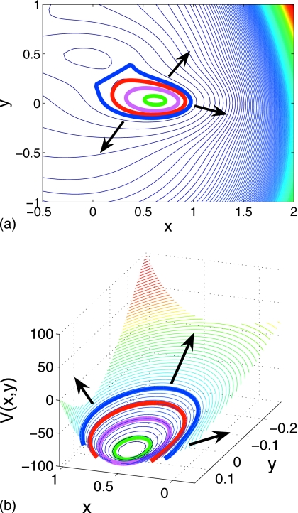
In such an arc-length stepping mode, the ring evolution for our potential (Fig. 7) is more robust to potential gradient nonuniformities. However, ring growth now does not couple to the actual topography of the landscape: In Fig. 7b it “sags” along the y-direction and there is considerable variation in potential values along any instantaneous ring.
Figure 7.
Arc length stepping on Müller–Brown potential with Δs=0.01 and N=80 (successive rings are shown at intervals of ten steps and arrows indicate direction of ring evolution).
Potential stepping
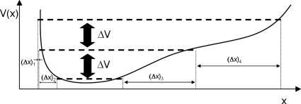
Evolving in constant potential steps enables the ring to directly track isopotential contours of the landscape. Potential stepping is shown schematically in one dimension in Fig. 8 for a potential minimum bracketed by a sharp incline on one side and a more gradual one on the other. A (reverse) step in the potential results in small variations in the x-variable [(Δx)1,(Δx)2] when the terrain is steep and in large x increments [(Δx)3,(Δx)4] when it is shallow. A qualitatively different approach is that of Laio and Parinello13 who employed a history-dependent bias as part of free energy surface searching that fills free energy wells; using repulsive markers actively prevents revisiting locations during further exploration. Irikura and Johnson45 used a combination of steps parallel and perpendicular to the energy gradient in a version of isopotential searching to identify chemical reaction products from a reactant configuration.
Figure 8.
Energy stepping in a smooth, asymmetric 1D energy well.
Here we directly transform the independent variable of the evolution equations using the chain rule
| (2.10) |
so that, as long as the quantity above is finite (e.g., away from critical points), the ring evolution equations now become
| (2.11) |
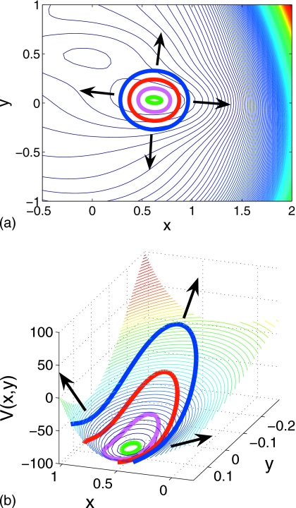
Note that FV(Φi,t)→∞ in regions where the potential is flat (dV∕dt→0); we impose an upper limit on the change in the variables Φi at each step of Eq. 2.11 when a threshold is exceeded. Potential-stepping ring evolution on the Müller–Brown potential is shown in Fig. 9: The ring rises in a balanced manner within the well and successive rings are indicative of the topology of the local landscape. The energy well is sampled evenly, tracking the potential contours. The almost linear segment of the ring visible in the final snapshot in Fig. 9a is formed as the ring approaches the (stable manifold of the) saddle point on the potential at (0.21,0.29); no further uphill motion, normal to the ring, is possible in this region. When such a situation is detected, one actively intervenes and modifies the evolution to assist the landscape search; examples of this will be given below.
Figure 9.
Potential stepping on Müller–Brown potential with ΔV=1.45 and N=80 (successive rings are shown at intervals of ten steps and arrows indicate direction of ring evolution).
Adjacent basins
The reverse integration for the example in Sec. 2B consisted in initialization close to the bottom of a single well, ring evolution uphill, and approach to the neighboring saddle point. We now discuss a reasonable strategy for transitioning between neighboring energy wells.
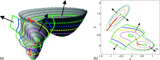
Figure 10 shows the results of reverse ring integration for three different initial rings, one close to the bottom of each of the wells of the Müller–Brown potential. Reverse integration here maps out the basin of attraction of each of the wells. For each initial condition, the reverse integration stalls in the vicinity of neighboring saddle points and ring nodes flow along the stable manifold of the corresponding saddle. As the ring nodes approach a saddle point the component of the energy gradient normal to the ring [(∇V(Φi))⊥] starts becoming negligible. To examine transitions between neighboring basins on the landscape we can employ global terrain methods33 that exploit the inherent connectedness of stationary points along valleys and ridges on the landscape. Figure 11 indicates the basins of attraction for each of the minima (identified using reverse integration) along with a red curve, which connects points that minimize the gradient norm along level curves of the potential (a MEP). This information is accumulated as the ring integration proceeds and suggests the direction to follow to locate neighboring minima. Upon detecting a local stagnation of ring evolution, caused by the approach to a saddle, a simple strategy is to (a) perform a local search for the saddle, through a fixed point algorithm, (b) compute the dynamically unstable eigenvector of this saddle, and (c) initialize a downhill search on the other side along this eigenvector away from the saddle point. This search for the nearby minimum may be through simple forward simulation or (in a global terrain context) by following points that minimize the gradient norm along level potential curves as above. This leads to the detection of a neighboring minimum, from which a new ring can be initialized and a further round of reverse integration performed. We reiterate that the procedure described so far (for purposes of easier exposition) is only for 2D, deterministic landscapes.
Figure 10.
Potential stepping on the Müller–Brown potential with ΔV=0.75 and N=160 [(successive (colored) rings are shown at intervals of ten steps]. Successive rings obtained by reverse integration starting from each of the minima on the landscape are shown.
Figure 11.
Potential stepping on Müller–Brown potential with ΔV=0.75 and N=160 [successive (colored) rings are shown at intervals of 30 steps]. Positions (red circles) of the minimum in gradient norm along the ring are shown at intervals of five steps in ring integration. Two different viewpoints of the same ring evolution are shown (consistent coloring of rings in each viewpoint). Black arrows indicate the direction of ring evolution out of each minimum. Left: Three-dimensional (3D) view; right: 2D overhead view (gray arrow indicates position of 3D view shown left).
ILLUSTRATIVE PROBLEMS FOR EFFECTIVE POTENTIAL SURFACES
In this section we present coarse reverse integration using effective potential stepping for two noisy problems: A Gillespie-type stochastic simulation algorithm (SSA) and a MD problem (alanine dipeptide in water). We assume that the problems we consider—in the regime we study them computationally—may be effectively modeled by the following bivariate SDE (all the examples studied are effectively 2D):
| (3.1) |
where v1(X) and v2(X) are drift coefficients, the diffusion matrix D is proportional to the unit matrix δij withDij=Dδij (a scalar matrix), where D is a constant, and W1t and W2t are independent Wiener processes. We previously considered (Sec. 2B) a deterministic example where numerical estimates for potential gradients were used to implement potential stepping. In the deterministic case, the drift coefficients are equal to minus the gradient of a potential V. For stochastic problems, such as those considered in this section, the drift coefficients are not so simply related to the gradient of an effective (generalized) potential (see Appendix C for additional discussion of this for 1D stochastic systems). In general, for reverse integration with steps in effective potential, we require estimates of all drift coefficients and all entries in the diffusion matrix (and even their partial derivatives). Here we discuss effective potential stepping for a system of the form given in Eq. 3.1 and also briefly discuss the general case where entries of the diffusion matrix are nonzero and dependent on X.
We assume Eq. 3.1 exists but is unavailable in closed form; estimates are therefore obtained by observing the process X and using v1(X)≡limΔt→0⟨[ΔX1]⟩∕Δt, v2(X)≡limΔt→0⟨[ΔX2]⟩∕Δt and 2D≡limΔt→0⟨[ΔX1]2⟩∕Δt=limΔt→0⟨[ΔX2]2⟩∕Δt. Here ΔXi=Xi(t+Δt)−Xi(t) and, by the form of Eq. 3.1, limΔt→0⟨ΔX1ΔX2⟩∕Δt=0. We note that the limit corresponds to Δt small but nonzero because the short bursts are short with respect to the time scale of the slow∕coarse variable but sufficiently long for equilibration of the remaining system variables. Additionally, the time step size required for accurate estimation of the drift coefficient differs from that required for the diffusion coefficient estimation.46, 47
These formulas, especially the ones for the drifts, suggest the construction of a useful coarse “pseudodynamical” evolution for our ring—a coarse evolution that follows the potential of mean force (PMF). The simplest version of these pseudodynamics evolves each point on the ring based on the local estimated drift—for the constant scalar diffusion mentioned above this evolution follows the PMF, and it becomes a true dynamical evolution at the deterministic limit.
For a black-box code implementing Eq. 3.1 this involves initializing at X, running an ensemble of realizations of the dynamics for a short time δt, estimating the local drift components of the SDE using the above formulas, performing a (forward or backward) projective step Δt in time [ΔXi=vi(X)Δt], and repeating the process. Further details of our estimation approach are provided in Appendix B.
We will argue that this accelerated pseudodynamical evolution (which we emphasize does not correspond to realizations of the SDE itself) can assist in the exploration of effective potential surfaces. The easiest approach would be to use reverse time stepping, or reverse arc length stepping in these pseudodynamics, and then (using formulas that will be discussed below and in Appendix C) finding the effective potential corresponding to each node visited. It is also possible, as we will see, to directly make upward steps in the effective potential; indeed, for the constant diffusion coefficient case we are studying, a proportionality exists between backward steps in time (for the pseudodynamics based on the drifts) and upward steps in the effective potential.
If the system in Eq. 3.1, with scalar diffusion matrix, has drift coefficients that satisfy the following potential condition:
| (3.2) |
it follows that the probability current vanishes at equilibrium, the drift coefficients (the time derivatives in our ring pseudodynamics) satisfy
| (3.3) |
and the difference in effective generalized potential (free energy) between a reference state and the state (X1,X2) may be directly computed from the following line integral:48
| (3.4) |
The analogy with the deterministic case [Eqs. 2.10, 2.11] carries through: The estimated drifts are proportional (via the constant D) to the effective potential gradients, and evolution following the drifts directly corresponds (modulo the proportionality constant) to evolution in the effective potential (PMF). Estimates of the local effective diffusion coefficients are typically necessary for exploration of the effective potential surface. We note that for a diagonal diffusion tensor with identical entries, Eq. 3.1, the size of the step βΔEeff is scaled [in Eq. 3.4] by the diffusion constant D. It follows that estimation of only the drift coefficients v1(X) and v2(X) allows us to perform reverse integration in our coarse dynamics [associated with the potential of mean force (PMF)]. A backward in time step Δt, leading to the state change ΔXi=vi(X)Δt, is, in effect, an “upward” step in the effective potential with the (unknown) scaled step size DβΔEeff. This approach is analogous to (and, in the appropriate limit will approximate) the deterministic potential stepping previously described (Sec. 2B). Here, for a stochastic problem, we need to additionally estimate diffusion coefficients to compute the potential change associated with each ring step uphill and, thereby, the effective free energy change associated with each ring.
For the general diffusion matrix D(X), with all entries possibly nonzero and dependent on X, we would compute the following partial derivatives of the effective potential:
| (3.5) |
| (3.6) |
and test whether the following potential condition is satisfied:48
| (3.7) |
If these potential conditions are satisfied then the effective generalized potential (free energy) may again be directly calculated from the following line integral:48
| (3.8) |
We do not consider the case when Eq. 3.7 does not hold; we refer the reader to Ref. 48.
In the same spirit with reverse ring stepping in potential (Sec. 2B), reverse ring stepping in effective potential may also be accomplished, subject to the stated assumptions, using the inner integrator as a black box: We run multiple replicas for particular initial conditions (the positions of nodes in the ring), observe (inner) forward time evolution, and, for a scalar diffusion matrix, use the estimated drifts and Eq. 3.4 to approximate changes in the effective potential numerically. We note that for a constant and isotropic diffusion tensor if we estimate only the drift coefficients we can still perform reverse ring stepping in the correct uphill direction and follow isopotential surfaces but the actual step size (and thus the actual value of the potential on the isopotential surfaces) will be unknown. As reverse ring integration proceeds, we store all calculated effective gradient values at each set of coarse-variable values, thereby building a database. Smoothed gradient estimates may be obtained for each ring node by using a weighted gradient average that includes estimates at nearby coarse-variable values in the database; we use kernel smoothing49 to select appropriate weights. For the more general case of state-dependent diffusion the drift dynamics do not simply correspond to dynamics in the effective potential [see Appendix C for corrections to dΦi∕dt required to retain the analogy to the deterministic equations 2.10, 2.11]. One could still employ the uncorrected drift dynamics as an ad hoc search tool (especially for problems close to scalar diffusion matrices) and postcompute the effective potential values the ring visits. In this case, however, the time parametrization of the effective potential evolution will not be meaningful and will even dramatically fail in the neighborhood of drift steady states that do not correspond to critical points in the effective potential (and vice versa).
A Gillespie-type SSA inner simulator example
The stochastic description of a spatially homogeneous set of chemical reactions, which treats the collisions of species in the system as essentially random events, is based on the chemical master equation.50 The Gillespie SSA is a MC procedure used to simulate a stochastic formulation of chemical reaction dynamics that accounts for inherent system fluctuations and correlations—this procedure numerically simulates the stochastic process described by the spatially homogeneous master equation.51 At each step in the simulation a reaction event is selected (based on the reaction probabilities), the species numbers updated (according to the stoichiometry of the reactions), and the time to the next reaction event computed. The reaction probabilities used in the algorithm are determined by the species concentrations and reaction rate constants as described in Ref. 51. The inner stochastic simulation routine we use here happens to employ an explicit tau-leaping scheme that takes larger time steps to encompass more reaction events while still ensuring that none of the propensity (reaction probability) functions in the algorithm changes significantly.52 The reaction events we simulate are chosen to implement a mechanism which, at the limit of infinitely many particles, would be described by the deterministic gradient system with potential V(x,y) defined as follows:
| (3.9) |
Consider the following deterministic rate equations:
| (3.10) |
| (3.11) |
This set of deterministic (coarse) rate equations may be written, for this problem, in the form of the following gradient system:
| (3.12) |
where x may be interpreted here as a vector of chemical species concentrations, and the potential energy function V*(x,y) is given by
| (3.13) |
with
| (3.14) |
Values for the rate constants are selected by requiring V*(x,y)=V(x−5,y−20) [i.e., V*(x,y) is selected as a shifted version of the V(x,y) from the previous example, with its fixed points in the positive xy quadrant, in an attempt to enforce positivity of the reaction probabilities required by the Gillespie algorithm]. The rate constant values chosen are k1=2960, k2=600, k3=40, k4=4783, k5=k6=1, and k7=15. This models the following hypothetical set of elementary reactions:
| (3.15) |
| (3.16) |
| (3.17) |
| (3.18) |
| (3.19) |
where species X (Y) has concentration x (y), the species T, U, V, and W are assumed to have unchanging concentration 1, and the reactions in Eqs. 3.17, 3.19 follow zeroth order kinetics.
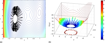
For the number of particles used in this Gillespie simulation, the drift coefficients estimated from the simulation practically coincide with the right-hand side of the deterministic rate equations, which happen to embody the gradient of the deterministic potential V(x,y) [Eq. 3.9]. The results of reverse ring integration up this deterministic potential, with drifts estimated from our Gillespie simulation, are shown in Fig. 12. The left panel shows nodal evolution over 100 rounds of reverse integration. In the right panel we superimpose the nodal evolution (with estimated potential indicated by color) on contours of the potential V(x,y) [defined in Eq. 3.9] for the deterministic gradient system in the form of Eq. 2.1. Since we are using an explicit tau-leaping Gillespie scheme, we do not have accurate estimates of the diffusion coefficients of the underlying chemical Fokker–Planck equation (FPE).53 For this problem these entries in the diffusion matrix cannot be well approximated as state independent, and a more involved process that includes their estimation is required in order to construct the true effective potential.
Figure 12.
Left: 100 rounds of drift potential-stepping ring evolution using an explicit tau-leaping inner Gillespie simulator with N=200; nodal redistribution is performed every ten reverse ring integration (coarse Euler) steps. The ring is initially centered at (−1,−1). Fifty replica Gillespie simulation runs are performed, each run with 10 000 particles and the explicit tau-leaping parameter ϵ=0.03. For the reverse integration ΔV=5×10⁻². Contours of the function V(x,y) [defined in Eq. 3.9] are shown. Right: 3D view of reverse ring integration shown left with estimated potential of each node shown according to the color bar. Evolving ring nodes with x<−1.2 are omitted for clarity. Contours of the function V(x,y) [defined in Eq. 3.9] are shown in 3D. Points on a single representative potential contour (as computed using reverse integration) are plotted as black symbols in the V(x,y)=−10 plane at the base of the figure; points along the actual potential contour are shown as red symbols.
Alanine dipeptide in water
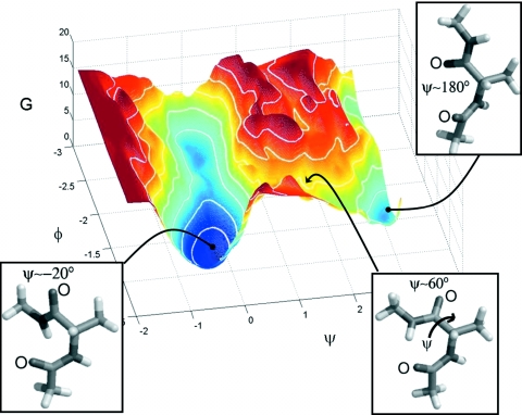
In this subsection we study the coarse effective potential landscape of alanine dipeptide (i.e., N-acetyl alanine N′-methyl amide) dissolved in water using coarse reverse (effective potential-stepping) integration. This system is a basic fragment of protein backbones with two main torsion angle degrees of freedom ϕ (C–N–Cα–C) and ψ (N–Cα–C–N), and with polar groups that interact strongly with each other and with the solvent. Extensive theoretical and experimental investigation of the alanine dipeptide has suggested good coarse observables (dihedral angles) for this system.54, 55, 56 Figure 13 shows the effective free energy landscape as a function of the dihedral angles ϕ and ψ of the alanine dipeptide. The structures of the alanine dipeptide in the α-helical (ψ=−0.3) and extended (ψ=π) states (corresponding to minima on the landscape) and at the transition state between them are also shown. We will use reverse integration on the effective potential energy landscape parametrized by these coarse coordinates. The coarse reverse integration is “wrapped around” a conventional forward-in-time MD simulator. It provides protocols for where (i.e., at what starting values of the coarse variables) to execute short bursts of MD, so as to map the main features of the effective potential surface (minima and connecting saddle points). These short bursts of appropriately initialized MD simulations provide [via estimation of the coefficients in Eq. 3.1] the deterministic and stochastic components of the alanine dipeptide coarse dynamics parametrized by the selected coarse variables. The current work assumes a diffusion matrix [Eq. 3.1] that is diagonal with identical constant entries. Our MD simulations of the alanine dipeptide in explicit water are performed using AMBER 6.0 and the PARM94 force field. The system is simulated at constant volume corresponding to 1 bar pressure, and the temperature is maintained at 300 K by weak coupling to a Berendsen thermostat. All simulations use a time step of 0.001 ps. The “true” effective potential here is the one obtained from the stationary probability distribution as approximated by a long MD simulation (24 ns).
Figure 13.
Free energy landscape for the alanine dipeptide in the ϕ-ψ plane (1kBT contour lines). Structures are shown corresponding to the right-handed α-helical minimum (left), the extended minimum (right), and the transition state between them (middle).
A preparatory “lifting” step is required at each reverse integration step for each ring node. Each coarse initial condition is lifted to many microscopic copies conditioned on the coarse variables ϕ and ψ. This step is not unique, since many configurations may be constructed having the same values of the coarse variables. Here we lift by performing a short MD run with an added potential Vconstr that biases (as in umbrella sampling) the coarse variables toward their target values (ψtarg,ϕtarg),
| (3.20) |
with kψ=kϕ=100 kcal mol−1 rad−1. The short lifting phase provides sufficient time for the fast variables to equilibrate following changes in the coarse variables. Following initialization we run and monitor the detailed MD simulations over short times (0.5 ps) and estimate, for each node in the coarse variables, the local drifts over multiple replicas. Each coarse backward Euler step of the ring evolution provides new coarse-variable values at which to initialize short bursts of the MD simulator. Each step in the reverse integration procedure consists of lifting from coarse variables (the coordinates of the ring nodes) to an ensemble of consistent microscopic configurations, execution of multiple short MD runs from such configurations, restriction to coarse variables, estimation of coarse drifts and diffusivities, and reverse Euler stepping of the ring in the chosen evolution mode.
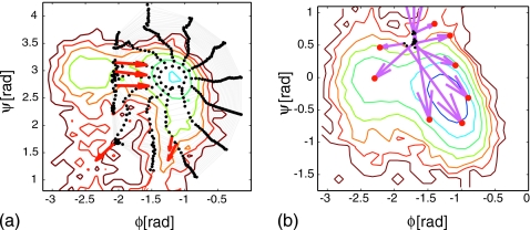
Figure 14 (left panel) shows ring nodes for 30 steps of reverse ring integration (using N=12 nodes) initialized around the extended structure minimum. Successive rings evolve up the well and are representative of the well topology. Reverse integration stalls, as expected, at the saddle points neighboring the extended structure minimum and identifies candidate saddle points in these regions. We note that, in the current context of (assumed) constant diffusion coefficients we can think of these saddles as steady states of the set of deterministic ODEs, coinciding with the drift terms of the effective Fokker–Planck. Then the “dynamically unstable” directions in a saddle (the downhill ones) are characterized by positive eigenvalues of the Jacobian of the drift equations; yet since these equations are proportional to the negative of the gradient of a potential, positive eigenvalues of the dynamical Jacobian correspond to negative eigenvalues of the Hessian. The eigenvectors associated with the unstable (for our PMF-related coarse dynamics) eigenvalue at these candidate saddles are also indicated in Fig. 14 and suggest the directions to dynamically follow to locate neighboring minima. We perturbed in the direction of the unstable eigenvector (associated with positive eigenvalue) away from one of the candidate saddle points and initialized (using a constrained potential, as before) multiple MD runs from this location. In Fig. 14 (right panel) we plot the observed evolution from these initial conditions down into the basin of the adjacent α-helical minimum.
Figure 14.
Alanine dipeptide ring integration. Left panel: Extended structure minimum: 30 rounds of reverse (coarse Euler) ring integration (number of ring nodes N=12) with scaled effective potential steps. Note that the scaled steps correspond to constant steps in free energy only if the effective diffusion tensor is diagonal with identical, constant entries, which appears to be a good approximation here. Eigenvectors corresponding to positive eigenvalues for candidate saddle points determined from ring integration are shown (long red arrows). Right panel: Downhill runs initialized at transition regions suggested by the reverse ring integration from the extended structure minimum. Initial conditions (black dots) are generated by umbrella sampling at a target coarse point selected by perturbation along the unstable eigenvector at the saddle. Final conditions for these downhill runs (red dots) suggest starting points for new rounds of reverse integration from adjacent minima. (1kBT contour lines used in both plots). Note that both wells are plotted rotated by 90° relative to Fig. 13.
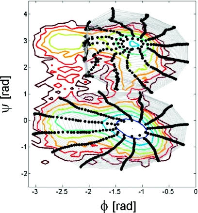
In Fig. 15 we show reverse ring evolution initialized close to both α-helical and extended minima. Clearly reverse ring evolution in this α-helical minimum well takes larger steps in ϕ, in which direction the effective potential is shallowest. We repeat that the reverse integration steps correspond to constant steps in free energy only if the effective diffusion tensor is diagonal and constant in both directions. The ring evolution shown in Fig. 15 appears to accurately track equal free energy contours suggesting that these assumptions (on the form of the diffusion tensor) may provide a suitable approximation here.
Figure 15.
Alanine dipeptide in water: 30 rounds of coarse reverse ring evolution (number of ring nodes N=12, DβΔEeff=0.05kBT) initialized in the neighborhood of both the right-handed α-helical minimum (bottom ring) and the extended minimum (top ring). Rings (gray lines) connecting nodes (black solid circles) are shown. Colored energy contours are plotted at increments of 1kBT.
SUMMARY AND CONCLUSIONS
We have presented a coarse-grained computational approach (coarse reverse integration) for exploration of low-dimensional effective landscapes. In our two-coarse-dimensional examples an integration (outer) scheme evolves a ring of replica simulations backward by exploiting short bursts of a conventional forward-in-time (inner) simulator. The results of small periods of forward inner simulation are processed to enable large steps backward in time (pseudotime in the stochastic case), in (phase space)×time or in potential in the outer integration. We first illustrated these different modes of reverse integration for smooth, deterministic landscapes. We extended the most promising approach for an illustrative deterministic problem, isopotential stepping, to relatively simple noisy (or effectively noisy) systems where closed-form evolution equations are not available. Simple estimation techniques were applied here to the results of appropriately initialized short bursts of forward simulation used locally to extract stochastic models with constant diffusion coefficients. Reverse integration in a single well and the approach to∕detection of neighboring coarse saddles was demonstrated. A brief discussion of global terrain approaches for exploring potential surfaces was included, along with a short demonstration of linking our approach to them. The main idea is to combine the computation of primary features of the energy landscape (saddles, minima) with more global mapping of the terrain in which they are embedded and the ability to progressively explore nearby basins and their connectivity.
We have presented here ring exploration using an effective potential using only estimation of the drift coefficients of our effective coarse model equations. Estimation of the diffusion coefficients (and their derivatives) is additionally required to quantitatively trace the effective potential surface. More sophisticated estimation techniques57, 58 allow for reliable estimation of both the stochastic and deterministic components of the coarse model equations. This permits a quantitative reconstruction of the effective free energy surface (and thereby the equilibrium density) using our reverse integration approach. The latter reconstruction is possible provided that the potential conditions discussed in Sec. 3 hold; testing this hypothesis should become an integral part of the algorithm.
In studies of high-dimensional systems, a central question is the appropriate choice of coarse variables used in the reverse integration. For high-dimensional systems, such as those arising in molecular simulations, the dynamics can typically be monitored only along a few chosen “coarse” coordinates. Formally, an exact evolution equation can be derived for these coordinates with the help of the projection-operator formalism,59 but that equation will be non-Markovian even if the time evolution in the full space is Markovian. To minimize the resulting memory effects, one can attempt to identify good (i.e., nearly Markovian) coordinates a priori, e.g., based on the extensive experience with the problem (as, say, in hydrodynamics) or by data analysis.60, 61 Alternatively, one can monitor the dynamics in a large space of trial coordinates and select a suitable low-dimensional space on the fly (e.g., from principal component analysis62). In general problems, where good coordinates are not immediately obvious, careful testing of the Markovian character of the projected dynamics on the time scale of the coarse forward or reverse integration will be an important component of the computation.61, 63
For the alanine dipeptide in water, we assumed that the effective dynamics could be described in terms of a few coarse variables known from previous experience with the problem: The two dihedral angles. We are also exploring the use of diffusion map techniques64 for data-based detection of such coarse observables, in effect trying to reconstruct Fig. 15 without previous knowledge of the dihedral angle coarse variables. An example of mining large data sets from protein folding simulations to detect good coarse variables using a scaled isomap approach can be found in Ref. 65; linking coarse variables with reverse integration for this example is discussed further in an upcoming publication.66 All the work in this paper was in two coarse dimensions. In the context of invariant manifold computations for dynamical systems (which provided the motivation for this work) more sophisticated algorithms exist for the computer-assisted exploration of higher-dimensional manifolds (as high as six dimensional).38, 39 It should be possible—and interesting!—to use these manifold parametrization and approximation techniques in combination with the approach presented here to test the coarse dimensionality of effective free energy surfaces one can usefully explore.
ACKNOWLEDGMENTS
This work was partially supported by DARPA Grant No. 31–1390–111–A and NSF Grant No. DMS-0504099, (T.A.F. and I.G.K.) and by the Intramural Research Program of the NIDDK, NIH (G.H.).
APPENDIX A: ARC LENGTH TRANSFORMATION RELATION
Consider a phase space-time arc length s that allows a projection
| (A1) |
The required transformation relation67 is
| (A2) |
with coordinates for node i. The transformed nodal evolution equation, with solution arc length as the independent variable, is given by
| (A3) |
where F is as defined in Eq. 2.6, and the ring boundary conditions remain periodic.
APPENDIX B: ESTIMATION
In the Gillespie case (Sec. 3A) we only allow ourselves to observe sample paths generated by the simulator which is treated as a black box (similarly for the MD simulator). A simple approach to estimating effective potential gradients (and eventually free energy gradients) is to perform sets of M-replica bursts of inner (Gillespie, MD) simulation initialized at each of the N ring nodes. For short replica simulation bursts (with n time steps), we can assume a local first order in time model68 for the mean (an n×2 matrix, with entries averaged using multiple replicas, rows corresponding to time abscissas, and columns corresponding to each coarse variable),
| (B1) |
where is an n×2 matrix, 1 is a vector of n ones, t is a vector of n time abscissas, ϵ is the n×2 matrix of model errors, and C is the 2×2 matrix of parameters computed (for each node) using least-squares estimation. The (pseudotime) derivative information (in the matrix C) is required, along with approximations of the tangent vectors at each node (ring geometry) to update the ring node positions in a reverse integration step; diffusion coefficients are also required, as discussed further below, to compute the relation between a reverse integration step size in pseudotime and the corresponding change in the effective potential. In the paper reverse ring time stepping is always meant in terms of the drift-based pseudodynamics (it only becomes true time stepping in the deterministic limit).
This derivative information may also be used to confirm the existence of an effective potential. For the case of two effective coarse dimensions, we locally compare, computing on a stencil of points, the X2-variation in dX1∕dt with the X1-variation in dX2∕dt (testing for equality of mixed partial derivatives of the effective potential). Alternatively, we may use a locally affine model for the drift coefficients of the following form:
| (B2) |
with A∊R2×2 and B∊R2, and employ maximum likelihood estimation techniques to obtain A and B (an effective potential exists provided A12=A21). In this context, recently developed maximum likelihood69 or Bayesian58 estimation approaches are particularly promising, allowing for simultaneous estimation of both the drift and diffusion coefficients. These approaches assume that the data are generated by a (multivariate) parametric diffusion; they employ a closed-form approximation to the transition density for this diffusion. For the case of a 1D diffusion process ,
| (B3) |
where Wt is the Wiener process, θ is a parameter vector, μ is the drift coefficient, and σ is the diffusion coefficient, the corresponding log likelihood function ln(θ) is defined as
| (B4) |
where n is the number of time abscissas, is the ith sample, and Δ is the time step between observations in the time series. The derivation of a closed-form expression for the transition density (and thereby the log likelihood function) allows for maximization of ln with respect to the parameter vector θ providing “optimal” estimates for the drift and diffusion coefficients associated with the time series. For higher-dimensional problems (such as the 2D ones considered here) see Ref. 57.
APPENDIX C: STATIONARY PROBABILITY DISTRIBUTION AND EFFECTIVE FREE ENERGY
We discuss here the effective potential [effective free energy Eeff(ψ)] we attempt to compute through reverse integration and its relation to the form of the stationary probability distribution Pst(ψ) for a 1D FPE.
In one dimension we write the FPE [with drift
| (C1) |
and diffusion coefficient
| (C2) |
where ψ(t;ψ0) is a sample path of duration t initialized at ψ0 when t=0] as follows:
| (C3) |
where the probability current S(ψ,t) is given by
| (C4) |
In one dimension, the stationary probability distribution corresponds to a constant probability current;48 for natural boundary conditions this constant is zero and stationary solutions of the FPE satisfy
| (C5) |
which is readily solved for (the logarithm of) Pst,
| (C6) |
The connection between the stationary probability distribution and the effective potential (effective free energy) for systems with a characteristic temperature/energy scale (given by the parameter β−1=kBT) is provided by the ansatz Pst(ψ)∝e−βEeff(ψ). Substitution of the ansatz into Eq. C6 gives
| (C7) |
In Sec. 3, after the fitting of model SDEs, we discussed the use of local estimates of the drift and diffusion coefficients in taking steps in some form of the effective potential for two example systems; we consider the basis of this approach here in one dimension. For the Gillespie problem of Sec. 3 reverse ring stepping results were compared to particular deterministic potentials V(ψ) [Eq. 3.9]. For the alanine dipeptide problem the results of reverse ring stepping were compared to an effective potential derived from the stationary probability distribution of the system (with the additional assumption of state-independent diffusion coefficients).
If, alternatively, we start from the Langevin equation
| (C8) |
where γ(ψ) is the friction coefficient, f0(ψ) is a deterministic force [minus the gradient of a deterministic potential function V(ψ)], is a drag force, and Γ(t) is the stochastic force, and take the high friction (overdamped) limit we obtain
| (C9) |
The fluctuation-dissipation relation connects (correlations of) the stochastic force to the drag force as follows:
| (C10) |
for a system at “temperature” T (energy scale kBT=β−1). Using Itô calculus we interpret Eq. C9 as
| (C11) |
with
| (C12) |
| (C13) |
This establishes a correspondence of the Langevin equation with the FPE in Eq. C3.
For the case of additive noise, where D(ψ)=D=const (implying [by Eq. C13] that γ(ψ)=γ=const), we find [by differentiation of Eq. C7 with respect to ψ] that the drift coefficient v(ψ) is simply related to the effective potential Eeff as follows:
| (C14) |
In this case, pseudodynamical reverse integration following drifts (as performed for the model SDE problem) coincides with stepping in effective potential (appropriately scaled with the constant diffusion coefficient). Using Eq. C12 in Eq. C14 we find
| (C15) |
For the case of multiplicative (state-dependent) noise the drift coefficient v(ψ) is not directly related to the gradient of the effective potential Eeff extracted from the equilibrium density; instead, it satisfies
| (C16) |
where
| (C17) |
with differing from βEeff by the state-dependent contribution ln D(ψ). For such systems with state-dependent noise we require (local) estimates of both drift and diffusion coefficients for effective potential stepping. These can be used in Eq. C7 [Eq. C17] to compute (differences in) the true effective potential Eeff (the “auxiliary” effective potential ),
| (C18) |
When temperature is not part of the problem description one considers the SDE
| (C19) |
which has the following stationary distribution:
| (C20) |
c being a normalization constant chosen such that . Local estimates of A(ψ) and B(ψ) can then, in a similar approach as above, be used to step backward in effective potential.
References
- Wolynes P. G., Onuchic J. N., and Thirumalai D., Science 267, 1619 (1995). 10.1126/science.7886447 [DOI] [PubMed] [Google Scholar]
- Kolossvary I. and Guida W. C., J. Am. Chem. Soc. 118, 5011 (1996). 10.1021/ja952478m [DOI] [Google Scholar]
- Brooks C. L., Onuchic J. N., and Wales D. J., Science 293, 612 (2001). [DOI] [PubMed] [Google Scholar]
- Wang F. and Landau D., Phys. Rev. Lett. 86, 2050 (2001). 10.1103/PhysRevLett.86.2050 [DOI] [PubMed] [Google Scholar]
- Huber T., Torda A., and van Gunsteren W., J. Comput. Aided Mol. Des. 8, 695 (1994). 10.1007/BF00124016 [DOI] [PubMed] [Google Scholar]
- Voter A. F., Montalenti F., and Germann T. C., Annu. Rev. Mater. Res. 32, 321 (2002). 10.1146/annurev.matsci.32.112601.141541 [DOI] [Google Scholar]
- Gear C. W., Kevrekidis I. G., and Theodoropoulos C., Comput. Chem. Eng. 26, 941 (2002). 10.1016/S0098-1354(02)00020-0 [DOI] [Google Scholar]
- Hummer G. and Kevrekidis I. G., J. Chem. Phys. 118, 10762 (2003). 10.1063/1.1574777 [DOI] [Google Scholar]
- Dellago C., Bolhuis P. G., Csajka F. S., and Chandler D., J. Chem. Phys. 108, 1964 (1998). 10.1063/1.475562 [DOI] [Google Scholar]
- Dellago C., Bolhuis P. G., and Chandler D., J. Chem. Phys. 108, 9326 (1998). [Google Scholar]
- Darve E. and Pohorille A., J. Chem. Phys. 115, 9169 (2001). 10.1063/1.1410978 [DOI] [Google Scholar]
- Chipot C. and Henin J., J. Chem. Phys. 123, 244906 (2005). 10.1063/1.2138694 [DOI] [PubMed] [Google Scholar]
- Laio A. and Parinello M., Proc. Natl. Acad. Sci. U.S.A. 99, 12562 (2002). 10.1073/pnas.202427399 [DOI] [PMC free article] [PubMed] [Google Scholar]
- van Erp T. S. and Bolhuis P. G., J. Comput. Phys. 205, 157 (2005). 10.1016/j.jcp.2004.11.003 [DOI] [Google Scholar]
- Baker J., J. Comput. Chem. 7, 385 (1986). 10.1002/jcc.540070402 [DOI] [Google Scholar]
- Taylor H. and Simons J., J. Phys. Chem. 89, 684 (1985). 10.1021/j100250a026 [DOI] [Google Scholar]
- Cerjan C. J. and Miller W. H., J. Chem. Phys. 75, 2800 (1981). 10.1063/1.442352 [DOI] [Google Scholar]
- Poppinger D., Chem. Phys. Lett. 34, 332 (1975). 10.1016/0009-2614(75)85665-X [DOI] [Google Scholar]
- Goto H., Chem. Phys. Lett. 292, 254 (1998). 10.1016/S0009-2614(98)00698-8 [DOI] [Google Scholar]
- Page M. and McIver J., J. Chem. Phys. 88, 922 (1988). 10.1063/1.454172 [DOI] [Google Scholar]
- Gonzalez C. and Schlegel H., J. Chem. Phys. 95, 5853 (1991). 10.1063/1.461606 [DOI] [Google Scholar]
- Ionova I. V. and Carter E. A., J. Chem. Phys. 98, 6377 (1993). 10.1063/1.465100 [DOI] [Google Scholar]
- Miron R. A. and Fichthorn K. A., J. Chem. Phys. 115, 8742 (2001). 10.1063/1.1412285 [DOI] [Google Scholar]
- Henkelman G. and Jonsson H., J. Chem. Phys. 111, 7010 (1999). 10.1063/1.480097 [DOI] [Google Scholar]
- Jonsson H., Mills G., and Jacobsen K. W., Classical and Quantum Dynamics in Condensed Phase Simulations (World Scientific, Singapore, 1998). [Google Scholar]
- Elber R. and Karplus M., Chem. Phys. Lett. 139, 375 (1987). 10.1016/0009-2614(87)80576-6 [DOI] [Google Scholar]
- Gillilan R. and Wilson K., J. Chem. Phys. 97, 1757 (1992). 10.1063/1.463163 [DOI] [Google Scholar]
- Henkelman G., Uberuaga B., and Jonsson H., J. Chem. Phys. 113, 9901 (2000). 10.1063/1.1329672 [DOI] [Google Scholar]
- Trygubenko S. and Wales D., J. Chem. Phys. 120, 2082 (2004). 10.1063/1.1636455 [DOI] [PubMed] [Google Scholar]
- E W., Ren W., and Vanden-Eijnden E., Phys. Rev. B 66, 052301 (2002). 10.1103/PhysRevB.66.052301 [DOI] [Google Scholar]
- E W., Ren W., and Vanden-Eijnden E., J. Phys. Chem. B 109, 6688 (2005). 10.1021/jp0455430 [DOI] [PubMed] [Google Scholar]
- Peters B., Heyden A., Bell A., and Chakraborty A., J. Chem. Phys. 120, 7877 (2004). 10.1063/1.1691018 [DOI] [PubMed] [Google Scholar]
- Lucia A., DiMaggio P. A., and Depa P., J. Global Optim. 29, 297 (2004). 10.1023/B:JOGO.0000044771.25100.2d [DOI] [Google Scholar]
- Lucia A. and Yang F., Comput. Chem. Eng. 26, 529 (2002). 10.1016/S0098-1354(01)00777-3 [DOI] [Google Scholar]
- Kevrekidis I. G., Gear C. W., and Hummer G., AIChE J. 50, 1346 (2004). 10.1002/aic.10106 [DOI] [Google Scholar]
- Rico-Martinez R., Gear C., and Kevrekidis I., J. Comput. Phys. 196, 474 (2004). 10.1016/j.jcp.2003.11.005 [DOI] [Google Scholar]
- Gear C. W. and Kevrekidis I. G., Phys. Lett. A 321, 335 (2004). 10.1016/j.physleta.2003.12.041 [DOI] [Google Scholar]
- Henderson M., Int. J. Bifurcation Chaos Appl. Sci. Eng. 12, 451 (2002). 10.1142/S0218127402004498 [DOI] [Google Scholar]
- Henderson M., SIAM J. Appl. Dyn. Syst. 4, 832 (2005). 10.1137/040602894 [DOI] [Google Scholar]
- Krauskopf B., Osinga H. M., Doedel E. J., Henderson M. E., Guckenheimer J., Vladimirsky A., Dellnitz M., and Junge O., Modeling and Computations in Dynamical Systems (World Scientific, Singapore, 2006). [Google Scholar]
- Johnson M. E., Jolly M., and Kevrekidis I. G., Numer. Algorithms 14, 125 (1997). 10.1023/A:1019104828180 [DOI] [Google Scholar]
- Guckenheimer J. and Worfolk P., Bifurcations and Periodic Orbits of Vector Fields (Kluwer Academic, Dordeecht, 1993). [Google Scholar]
- Ren W., Commun. Math. Sci. 1, 377 (2003). [Google Scholar]
- Müller K. and Brown L. D., Theor. Chim. Acta 53, 75 (1979). 10.1007/BF00547608 [DOI] [Google Scholar]
- Irikura K. and Johnson R., J. Phys. Chem. A 104, 2191 (2000). 10.1021/jp992557a [DOI] [Google Scholar]
- Gradisek J., Siegert S., Friedrich R., and Grabec I., Phys. Rev. E 62, 3146 (2000). 10.1103/PhysRevE.62.3146 [DOI] [PubMed] [Google Scholar]
- Yates C., Erban R., Escudero C., Couzin I., Buhl J., Kevrekidis I., Maini P., and Sumpter D., Proc. Natl. Acad. Sci. U.S.A. 106, 5464 (2009). [DOI] [PMC free article] [PubMed] [Google Scholar]
- Risken H., The Fokker-Planck Equation: Methods of Solutions and Applications, Springer Series in Synergetics, 2nd ed. (Springer, New York, 1996). [Google Scholar]
- Wand M. P., Kernel Smoothing, Monographs on Statistics and Applied Probability (Chapman and Hall, London, 1995). [Google Scholar]
- McQuarrie D. A., J. Appl. Probab. 4, 413 (1967). 10.2307/3212214 [DOI] [Google Scholar]
- Gillespie D., J. Phys. Chem. 81, 2340 (1977). 10.1021/j100540a008 [DOI] [Google Scholar]
- Gillespie D., J. Chem. Phys. 115, 1716 (2001). 10.1063/1.1378322 [DOI] [Google Scholar]
- Cao Y., Petzold L. R., Rathinam M., and Gillespie D. T., J. Chem. Phys. 121, 12169 (2004). 10.1063/1.1823412 [DOI] [PubMed] [Google Scholar]
- Rossky P. J. and Karplus M., J. Am. Chem. Soc. 101, 1913 (1979). 10.1021/ja00502a001 [DOI] [Google Scholar]
- Brooks C. L. and Case D. A., Chem. Rev. (Washington, D.C.) 93, 2487 (1993). 10.1021/cr00023a008 [DOI] [Google Scholar]
- Chipot C. and Pohorille A., J. Phys. Chem. B 102, 281 (1998). 10.1021/jp970938n [DOI] [PubMed] [Google Scholar]
- Ait-Sahalia Y., “Closed-form likelihood expansions for multivariate diffusions,” NBER Working Paper No. W8956, 2002. Available at SSRN: http://ssrn.com/abstract=313657.
- Hummer G., New J. Phys. 7, 34 (2005). 10.1088/1367-2630/7/1/034 [DOI] [Google Scholar]
- Zwanzig R., Nonequilibrium Statistical Mechanics (Oxford University Press, New York, 2001). [Google Scholar]
- Nadler B., Lafon S., Coifman R. R., and Kevrekidis I. G., Appl. Comput. Harmon. Anal. 21, 113 (2006). 10.1016/j.acha.2005.07.004 [DOI] [Google Scholar]
- Best R. B. and Hummer G., Proc. Natl. Acad. Sci. U.S.A. 102, 6732 (2005). 10.1073/pnas.0408098102 [DOI] [PMC free article] [PubMed] [Google Scholar]
- García A. E., Phys. Rev. Lett. 68, 2696 (1992). 10.1103/PhysRevLett.68.2696 [DOI] [PubMed] [Google Scholar]
- Hummer G., Proc. Natl. Acad. Sci. U.S.A. 104, 14883 (2007). 10.1073/pnas.0706633104 [DOI] [PMC free article] [PubMed] [Google Scholar]
- Coifman R., Lafon S., Lee A., Maggioni M., Nadler B., Warner F., and Zucker S., Proc. Natl. Acad. Sci. U.S.A. 102, 7426 (2005). 10.1073/pnas.0500334102 [DOI] [PMC free article] [PubMed] [Google Scholar]
- Das P., Moll M., Stamati H., Kavraki L. E., and Clementi C., Proc. Natl. Acad. Sci. U.S.A. 103, 9885 (2006). 10.1073/pnas.0603553103 [DOI] [PMC free article] [PubMed] [Google Scholar]
- Das P., Frewen T. A., Kevrekidis I. G., and Clementi C. (unpublished).
- Kubicek M. and Marek M., Computational Methods in Bifurcation Theory and Dissipative Structures (Springer-Verlag, New York, 1983). [Google Scholar]
- Draper N. R. and Smith H., Applied Regression Analysis, Wiley Series in Probability and Mathematical Statistics (Wiley, New York, 1981). [Google Scholar]
- Ait-Sahalia Y., Econometrica 70, 223 (2002). 10.1111/1468-0262.00274 [DOI] [Google Scholar]


