Inferring the Strength of Selection in Drosophila under Complex Demographic Models

Abstract

Transposable elements (TEs) constitute a substantial fraction of the genomes of many species, and it is thus important to understand their population dynamics. The strength of natural selection against TEs is a key parameter in understanding these dynamics. In principle, the strength of selection can be inferred from the frequencies of a sample of TEs. However, complicated demographic histories, such as found in Drosophila melanogaster, could lead to a substantial distortion of the TE frequency distribution compared with that expected for a panmictic, constant-sized population. The current methodology for the estimation of selection intensity acting against TEs does not take into account demographic history and might generate erroneous estimates especially for TE families under weak selection. Here, we develop a flexible maximum likelihood methodology that explicitly accounts both for demographic history and for the ascertainment biases of identifying TEs. We apply this method to the newly generated frequency data of the BS family of non-long terminal repeat retrotransposons in D. melanogaster in concert with two recent models of the demographic history of the species to infer the intensity of selection against this family. We find the estimate to differ substantially compared with a prior estimate that was made assuming a model of constant population size. Further, we find there to be relatively little information about selection intensity present in the derived non-African frequency data and that the ancestral African subpopulation is much more informative in this respect. These findings highlight the importance of accounting for demographic history and bear on study design for the inference of selection coefficients generally.

Introduction

Transposable elements (TEs) are present in the genomes of virtually every species studied (Hua-Van et al. 2005), in many instances contributing a substantial fraction of overall genome size (Biemont and Vieira 2006). Although thought of as primarily genomic parasites (Charlesworth and Langley 1989), TEs also play an important role in the evolution and function of genes and genomes (Kazazian 2004; Volff 2006). TEs can generate chromosomal rearrangements, such as inversions and duplications, that contribute to the structural evolution of genomes. Some TEs have been “domesticated” by their host genome, serving either as genes or regulatory elements (Medstrand et al. 2005; Volff 2006). For example, in Drosophila, telomere maintenance depends on recently domesticated TEs (Casacuberta and Pardue 2002). TEs sometimes carry host gene sequences with them as they transpose, which suggests their involvement in exon shuffling and gene duplication (Moran et al. 1999). Understanding the functional roles, evolution, and population dynamics of TEs is therefore essential to a full understanding of genome evolution and function.

In Drosophila, TEs are often maintained at low population frequencies, suggesting that they are generally deleterious (Charlesworth and Langley 1989; Charlesworth et al. 1994). The spread of TEs is likely to be limited both by regulation of transposition rate and by natural selection against individual TE copies (Charlesworth and Langley 1989). Several distinct modes of selection acting to stabilize element copy number have been proposed (Nuzhdin 1999). These include selection against insertion into coding sequences, selection against the deleterious effects of ectopic recombination among dispersed TE copies, and selection against the translation of TE-encoded proteins (Montgomery et al. 1987; McDonald et al. 1997; Petrov et al. 2003). Petrov et al. (2003) quantified the intensity of selection against four families of non-long terminal repeat retrotransposons in D. melanogaster, using North American TE frequency data within a maximum likelihood (ML) framework. Their estimate of the intensity of selection was based on frequency data from derived populations only and did not account for the demographic history of the species.

If non-African populations of D. melanogaster have experienced a recent, intense bottleneck as has been suggested (Li and Stephan 2006; Thornton and Andolfatto 2006), then many of the TEs segregating in the ancestral, prebottleneck population should have been lost or have otherwise changed their frequency substantially during the bottleneck, altering the overall element frequency distribution. These effects should be of minor importance for TE families that are subject to very strong purifying selection because many TEs in such families will be younger than the bottleneck and thus should not be affected by it. However, for the families under weak purifying selection with more frequent and thus old TE copies, the bottleneck might have a profound effect. Specifically, it should erase signatures of weak selection, making these TE families appear neutral.

Here, we describe an ML procedure that allows estimation of selection intensities in the ancestral population while accounting both for the bottleneck and for the ascertainment biases. We apply this method for two recently proposed demographic models for the emigration of D. melanogaster out of Africa (Li and Stephan 2006; Thornton and Andolfatto 2006). The framework can be easily extended to other bottleneck models as long as the population can be assumed to have been at equilibrium at some specific point in the past in the ancestral population. We then reanalyze the population dynamics for TEs from the BS family, a LINE-like TE family that was one of the four families studied in Petrov et al. (2003). Additional frequency data were obtained for 18 BS elements in four North American and four African populations.

We find that incorporating the demographic models of Thornton and Andolfatto (2006) and Li and Stephan (2006) yields quite different estimates of the strength of selection than those obtained assuming a randomly mating population of constant size. In particular, we find that there remains very little information with which to infer the strength of selection from North American frequency data alone when demography is taken into account. The African frequency data, by contrast, is relatively informative about Ns, and we estimate that the ancestral strength of purifying selection against the BS family was Ns ≈ −4. We are also able to reject the hypothesis that this family has evolved under neutrality.

Materials and Methods

Polymerase Chain Reaction (PCR) Assays to Check for the Presence/Absence of BS Elements

In total, 89 different D. melanogaster strains were used in this study: Forty-six strains are from 4 different populations in North America, and 43 strains are from 4 different populations in Africa. Further details on the strains are provided in supplementary table S1, Supplementary Material online. Genomic DNA from all these strains was extracted using a DNeasy Tissue kit (Qiagen, Valencia, CA).

The presence/absence of the 29 BS elements annotated in release 3.0 of the D. melanogaster reference sequence (Kaminker et al. 2002) was assayed in both North American and African populations. DNA from the North American subpopulation was combined into a total of 5 pools of 8 or 10 strains. DNA from the African subpopulation was combined into a total of 4 pools of 9, 11, or 12 strains. The final concentration of each pool was 2.5 ng of DNA of each individual strain per PCR reaction. This DNA concentration was previously verified in our laboratory to be sufficient to detect the presence of a TE in a single strain out of the total number of strains tested in the pool (Lipatov et al. 2005). The composition of each pool is given in supplementary table S1, Supplementary Material online. When the element was present in a pool, we assayed for the presence of the element for each strain in that pool individually using PCR. For some of the pools, single-strain PCRs were performed even though the pooled PCR indicated that the element was absent.

Primers for each of the 29 BS elements were designed in the sequenced strain of D. melanogaster (y¹; cn¹ bw¹ sp¹) using the program Primer3 (http://primer3.sourceforge.net/). Two primer sets were designed for each of the elements (supplementary table S2, Supplementary Material online). The first primer set was intended to assay for the presence of the element; each pair of primers in this set consists of a “Left” primer that lies within the BS element sequence and a “Right” primer that lies in the flanking region to the right of the insertion. This PCR should yield a product only when the element is present. Each pair in the second primer set consists of a “Flanking” primer designed to anneal to the flanking region to the left of the element and the Right primer used before. The PCR with these primers is expected to yield a product only when the element is absent. PCRs were run using REDTaq DNA polymerase (Sigma, St Louis, MO). The PCR conditions for both reactions were: 94 °C for 2 min, 13 cycles of 94 °C for 0.5 min, 63 °C for 0.5 min (−0.5 °C per cycle), 72 °C for 1 min, and then 20 cycles of 94 °C for 0.5 min, 56 °C for 0.75 min, 72 °C for 1 min, and one last extension step of 10 min at 72 °C. For one element, specific primers could not be designed because the regions flanking the insertion were repetitive. For five other elements, R5.9 of the D. melanogaster genome revealed that one or both of the primers flanking the insertion were designed inside another TE. Consequently, the results for these five TEs were discarded. Three elements were not present in any of the pools, and two further elements were fixed in all pools, leaving 18 of the 29 elements.

Demographic Models for D. melanogaster

Two demographic models for the emigration of D. melanogaster out of Africa have recently been proposed (Li and Stephan 2006; Thornton and Andolfatto 2006). They are illustrated in figure 1. The models assume that an ancestral population split into two subpopulations at the time of emigration t_b with no further migration between them afterward. In the following, we will refer to the ancestral population as “African” and the derived population as “North American.”

FIG. 1.—

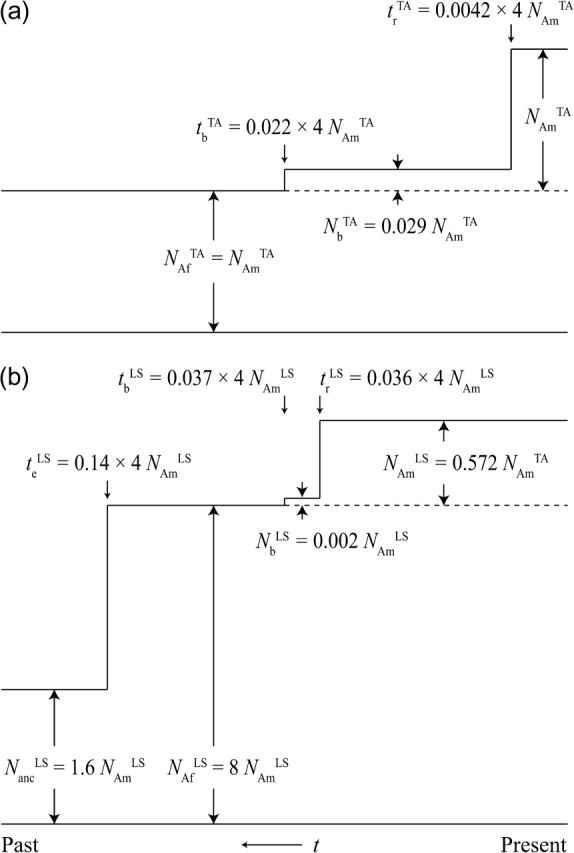
The two demographic models used: (a) Thornton and Andolfatto (2006) and (b) Li and Stephan (2006). In both models, North American (above dashed line) and African (below dashed line) subpopulations split at time t_b, followed by a population bottleneck in North America that lasted until t_r. The LS model additionally features an ancient population expansion in Africa.

Both models state that emigration was associated with a severe population bottleneck in the new North American subpopulation. The initial population size N_b of the North American subpopulation at the time of emigration was considerably smaller compared with the size N_Af of the ancestral African population. The bottleneck lasted until a recovery time t_r at which the North American subpopulation instantaneously expanded to its present size N_Am. Whereas in the demographic model of Thornton and Andolfatto (2006) (TA) the size of the African population N_Af is assumed to have remained constant throughout its entire history, the model of Li and Stephan (2006) (LS) postulates an ancient population size expansion of the African population that occurred at a time t_e long prior to the emigration event. During this expansion, the African population instantaneously increased from an ancient size N_anc to its present-day size N_Af. Due to the additional incorporation of an ancient population expansion, the LS model is clearly more complex compared with the TA model and serves us as an instructive example of how such expansions can generally be incorporated into our methodology.

The TA model is described by five parameters N_Af^TA, N_b^TA, N_Am^TA, t_b^TA, and t_r^TA. The LS model requires two additional parameters for the ancient population expansion in Africa and hence is determined by seven parameters N_anc^LS, N_Af^LS, N_b^LS, N_Am^LS, t_e^LS, t_b^LS, and t_r^LS. The particular values used for our analysis are stated in figure 1 and resemble the original values derived in Thornton and Andolfatto (2006) and Li and Stephan (2006). For reasons of comparability between the two models, the values for the LS model were rescaled according to the procedure described in Macpherson et al. (2008). Notice that in addition to the ancestral population expansion, which is exclusive to the LS model, both models also differ considerably in their bottleneck parameters and the values for present-day population sizes in Africa and North America. For example, the bottleneck of the TA model is longer but less severe than the bottleneck of the LS model, and the present-day size of the African subpopulation in the LS model is almost 5-fold larger than that in the TA model.

ML Estimation Procedure

In the following, we will describe an ML approach for inferring the selection coefficient of a TE family that explicitly takes into account demographic history and ascertainment bias. To compute the likelihood of an observed set of TE frequency pairs in the African and North American subpopulations for a given selection coefficient, we require knowledge about the expected distribution of such frequencies. We will derive these distributions from forward Wright–Fisher simulations of TE frequency trajectories for the two demographic models specified above.

TE insertions in the African population are modeled according to the infinite-sites model, and different TE copies are considered to evolve independently of each other. We restrict our analysis to TEs that originally transposed prior to the time of emigration. We also assume that TEs were initially found in a single inbred strain from North America. Other ascertainment schemes can be easily implemented as well.

Individuals homozygous for a TE have fitness 1 + s, heterozygotes have fitness 1 + s/2, and individuals without the element have fitness 1. We assume that the selection coefficient s remained constant in the African subpopulation throughout its history, whereas it became zero for TEs in the North American subpopulation after the population split. The latter assumption is clearly valid during the bottleneck, where effective population size, and thus effectiveness of selection, is substantially reduced. There is also strong reason to assume that s remained close to zero in the North American population after the bottleneck. As will be shown later in the manuscript, the expected number of heterozygous BS sites in a diploid genome is much lower in North American individuals than in individuals from Africa because many low-frequency BS elements have been lost during the bottleneck. Ectopic recombination between dispersed TEs copies will therefore occur less frequently in individuals from the derived population compared with the ancestral population. As such ectopic recombination events are considered to be the major cause for selection against BS elements (Montgomery et al. 1987; Petrov et al. 2003), we expect the strength of purifying selection against BS elements to be substantially reduced in the derived population.

Our method assumes that at some point prior to the emigration of the North American subpopulation, TEs were at transposition–selection equilibrium in the African population. In the TA model, this can be assumed at all times because the size of the African population remained constant throughout its history, and we do not take into account temporal variation in transposition rates or selection coefficients in Africa. Thus, African TE frequencies should, in particular, also be at transposition–selection equilibrium at the time of emigration t_b. In the LS model, however, this need not be the case due to the ancient expansion of the African population. The instantaneous expansion might have driven the distribution of TE frequencies out of transposition–selection balance to such an extent that equilibrium has still not been re-established at the time of emigration. We therefore assume that transposition–selection equilibrium holds in the African population only up to time t_e in the LS model.

The expected number of polymorphic sites at frequency x in transposition–selection equilibrium and for the infinite-sites model has been derived by Sawyer and Hartl (1992) in a Poisson Random Field framework. If μ is the rate at which TEs transpose in an individual genome per generation, then for a given population size N and selection coefficient s the average number of polymorphic sites that are present at frequency x in the population can be approximated by

(1)

where x∈{1/(2N),2/(2N),…,1 − 1/(2N)}. Dividing g(x, μ, Ns) by the expected overall number of polymorphic sites yields the normalized distribution of TE frequencies at these sites,

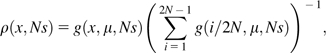(2)

which becomes independent of μ. Notice that this result coincides with the distribution derived in Nagylaki (1974) and Petrov et al. (2003), where a slightly different approach was used.

In the TA model and for a given selection coefficient s, the probability that a randomly chosen polymorphic site has frequency x_b in the African population at time t_b is hence simply given by

(3)

In the LS model, we lack an analytic expression for the distribution of TE frequencies in Africa after the population expansion. Equation (2) does not apply here because TE frequencies cannot be assumed to obey transposition–selection equilibrium. Creating a random ensemble of TE frequencies at the time of the split t_b therefore requires additional effort and will be described in the following.

Polymorphic TEs present at the time of the population split t_b can be subdivided into two classes: The first class are TEs that resulted from a new transposition event in a single individual after the expansion. Their initial frequency is x₀ = 1/(2N_Af^LS), and transposition times t₀ can assumed to be uniformly distributed throughout the interval (t_e, t_b). On average, we expect 2μN_Af^LS(t_e − t_b) new transpositions to have occurred between t_e and t_b. The second class are elements that were already present at the time of the ancient population expansion. As stated above, we assume that the frequencies of those TEs were at transposition–selection equilibrium prior to the expansion. According to equation (1), the expected number of polymorphic sites at frequency x in the population at time t_e was therefore g(x,μ,N_anc^LSs). The instantaneous population expansion does not change this function for frequencies x∈𝒳_anc = {1/(2N_anc^LS),2/(2N_anc^LS),…,1 − 1/(2N_anc^LS)} because we assume that expansion occurred in an entirely uniform fashion (i.e., the number of individuals that carry a particular allele was increased by the same factor N_Af^LS/N_anc^LS for all alleles and at all polymorphic sites). Notice that according to this procedure, TEs could not have been present at any other frequency x∉𝒳_anc immediately after the expansion.

Combining the two classes, we can set up a well-defined probabilistic model for the ensemble of candidate sites from which all sites polymorphic at the split must have originated. Each element of this ensemble is specified by its initial frequency x₀ and starting time t₀. We can draw a random member of the ensemble by first choosing its initial frequency x₀ from

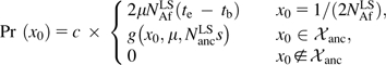(4)

with normalization factor c = 1/[2μN_Af^LS(t_e − t_b) + ∑_x0∈𝒳ancg(x₀,μ,N_anc^LSs)]. The probability density distributions for starting times t₀ ∈ [t_b, t_e] conditional on the initial frequency x₀ is then

(5)

using Dirac's delta function . For the LS model, the probability that a polymorphic site drawn randomly from the African population at time t_b has frequency x_b is therefore given by

(6)

where Pr[x_b, t_b | x₀, t₀, N_Af^LS, s] is the transition probability (x₀, t₀) → (x_b, t_b) under the Wright–Fisher model with selection coefficient s and population size N_Af^LS. For our simulations, we do not require explicit knowledge of the full distribution Pr^LS(x_b). We only need to be capable of drawing random elements from it. This can easily be achieved by first drawing a candidate (x₀, t₀) from equations (4) and (5), evolve it through the African population by binomial sampling with selection coefficient s and population size N_Af^LS until time t_b, and record its frequency x_b. If the candidate becomes fixed or lost prior to time t_b, we draw a new candidate.

In the previous paragraphs, we have described for both demographic models how random allele frequencies can be obtained from the frequency distribution of polymorphic sites in the population at the time of the split. A numerically efficient implementation is achieved by creating lookup tables (Knuth 1997) for the distributions (3) and (4). The randomly drawn frequencies x_b at time t_b serve us as starting points for the simulation of frequency trajectories in the North American and African subpopulations, from which the probability distributions for present-day TE frequencies can be derived. We simulate these trajectories for a given selection coefficient s and a chosen demographic model (TA or LS) according to the following procedure:

1. Draw a random allele frequency x_b at the time of the split from the probability distribution (3) for the TA model or distribution (6) for the LS model, respectively.

2. Iterate the allele frequency forward from t_b through the bottlenecked (North American) subpopulation by binomial sampling with s = 0 according to the chosen demographic model until fixation or loss occurs or t_b generations have elapsed, that is, the present generation has been reached.

3. If the allele has been lost, return to step 1 (lost alleles will not be observed as they cannot have been ascertained in the initially sequenced North American strain). Otherwise, denote the allele frequency reached at the present day in North America x_Am and continue.

4. Sample u from Uniform(0, 1). If x_Am < u, reject x_Am and return to step 1.

5. Iterate from x_b forward through the African subpopulation by binomial sampling according to the chosen demographic model with selection coefficient s until fixation or loss occurs or t_b generations have elapsed. Denote the present-day African allele frequency x_Af.

6. Record initial frequency x_b and subpopulation frequencies x_Am and x_Af.

The implementation of the iteration procedures specified in steps 2 and 5 was checked by comparison of the probabilities of fixation and loss obtained by simulation to their respective asymptotic analytical values, given by equations (5.28) and (5.29) in Ewens (2004). Ascertainment bias arising from the sampling scheme is incorporated in steps 3 and 4 of the above procedure. The probability that an element segregating at frequency x_Am is present in the reference sequence is simply x_Am. Note that the sampling scheme can affect the distributions of both North American and African elements because in step 5 we can only begin from an x_b corresponding to an element that has been observed to be either polymorphic or fixed in the North American subpopulation. A different ascertainment bias can be incorporated by changing steps 3 and 4 appropriately.

For the TA model, we repeat the simulation procedure until a list with 10⁵ triplets (x_b, x_Am, x_Af) is obtained for each investigated selection coefficient s. Because the LS model is substantially more demanding in terms of the runtime required to draw an initial frequency x_b, only 10⁴ triplets are generated for this model for each s. From the simulation results, we can derive numerical approximations for the expected probability distributions of TE frequencies in the present-day African and North American subpopulations. Knowledge of these distributions then allows us to calculate likelihoods of our set of observed TE frequencies. For a given demographic model and selection intensity Ns, we have

(7)

where kⁱ is the number of strains bearing the ith TE among nⁱ genotyped strains in each subpopulation, and m is the number of different TEs investigated in our analysis. The probability P_i of observing {k_Amⁱ, n_Amⁱ, k_Amⁱ, n_Amⁱ} for a particular TE is given by

(8)

The two-dimensional distribution ϕ(x_Am, x_Af | Ns) is the expected probability density of observing a frequency pair (x_Am, x_Af), and B_x(k | n) are binomial distributions that incorporate the effects of sampling from a finite number of genotyped strains.

For both investigated demographic scenarios, it turns out that ϕ(a, b) can be well approximated by the product ϕ_Am(a) × ϕ_Af(b) of the individual one-dimensional probability distributions in the African and North American subpopulations. The reason this factorization works is that correlation between allele frequencies x_b at the time of emigration and present-day frequencies x_Am in North America is substantially diminished during the bottleneck, as shown in figure 2. This finding does not imply that the expected distribution ϕ_Af is actually unaffected by the bottleneck and could therefore be simply obtained by evolving the allele frequency distribution Pr(x_b) in Africa from t_b to the present. The bottleneck still has a profound influence on ϕ_Af due to the fact that the probability for an allele to “survive” the bottleneck clearly depends on its frequency x_b at emigration, and we condition the distribution of allele frequencies in Africa on those TEs that have not become lost during the bottleneck in the North American subpopulation.

FIG. 2.—

Loss of correlation between allele frequencies x_b at the time of emigration and present-day frequencies x_Am in North America during the bottleneck. The plots show 10³ simulated frequency pairs (x_b, x_Am) and (x_b, x_Af) for both the TA model and LS model, using each model's ML estimate for Ns in the African population. Pearson product–moment correlation coefficients for pairs (x_b, x_Am) are r = 0.18 in the TA model and r = 0.26 in the LS model. Frequency pairs (x_b, x_Af), in contrast, are still strongly correlated (TA: r = 0.92, LS: r = 0.99).

We numerically approximate the expected frequency distributions ϕ_Am/Af (x) by binning all frequencies x_Am ∈ (0, 1) and x_Af ∈ (0, 1) obtained from our simulations for a given demographic model and selection coefficient into 100 successive bins of equal width Δ = 0.01. For each bin j∈{1,2,…,100}, the number of elements in this bin is divided by the overall number of simulation runs to obtain ϕ(j), that is, the probability of observing a frequency that falls within bin j. ϕ(0) and ϕ(101) denote the probabilities of observing lost and fixed TEs, respectively. Notice that ϕ_Am(0) will always be zero as lost elements cannot be observed for the North American population. From the binned distributions, we can finally calculate individual likelihoods according to

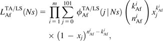(9)

where x_j = Δ × (j − 1/2) is the midpoint of bin j. Likelihoods L_Am^TA/LSare derived analogously. Combined likelihoods for both subpopulations are then obtained by the products

(10)

In our calculation of likelihoods (9), we sum over all bins of the numerically estimated distributions ϕ_Am/Af (x), where each bin is weighted according to a binomial distribution centered around the observed TE frequency x_j. Stochastic fluctuations between neighboring bins are therefore effectively smoothed out, making the likelihood estimation considerably robust to changes in binning resolution. We checked that a more coarse-grained binning with only 10 bins, for example, does not alter our results (data not shown). We also verified that calculated likelihoods rapidly converge with increasing number of simulation runs (data not shown). The numbers of bins and simulation runs used in our analysis are fully sufficient to obtain reliable results.

The simulation algorithm was implemented in C++. Runs were performed on up to 200 CPUs of the Bio-X² cluster at Stanford University. The resulting data were analyzed using a combination of Perl and R programs. All software is available from the corresponding author upon request.

Results and Discussion

Estimation of Selection Coefficients Using the ML Procedure

The frequency data obtained from genotyping the individual members of the BS family in our experimental data set are summarized in table 1. Six of the 18 genotyped elements are present in the North American population but were not observed in any of the African pools. In principle, these elements could have transposed in North America after the emigration and thus would not be suitable for consideration in our analysis. This, however, is highly unlikely because all six elements are observed at moderate to high frequency in North America. Presumably they originated from TEs that were present at low-frequency in the African population at the time of emigration yet subsequently increased in frequency during the bottleneck. We therefore kept these six elements for our analysis.

Table 1.

Genomic and Population Data for the 18 BS Elements Studied

				African							North American
Flybase ID	La	rb	Armc	MW	Zmel	KY	ZW	kAfd	nAfe	xAff	Wi	We1	We2	NB	CSW	kAmd	nAme	xAmf
FBti0018877	130	1.69	2R	0/11	0	0/11	0	0	41	0.00	0	2/10	2/9	4/8	3/7	11	43	0.26
FBti0018878	128	2.23	2R	1/9	0/8	2/9	0/9	3	35	0.09	0/9	0/7	0/9	1/8	0	1	40	0.03
FBti0018879	136	3.47	2R	0/8	0/9	0/11	0/11	0	39	0.00	6/10	4/9	6/8	5/8	5/8	26	43	0.60
FBti0019079	473	2.51	X	2/10	0	0	4/12	6	40	0.15	4/10	1/10	2/9	3/7	3/7	13	43	0.30
FBti0019133	125	3.98	2L	0/9	2/8	4/11	1/11	7	39	0.18	7/10	7/10	2/10	4/8	2/7	22	45	0.49
FBti0019158	144	3.01	2L	1/11	2/9	4/11	0/12	7	43	0.16	1/9	1/10	4/9	0	0	6	43	0.14
FBti0019165	2326	2.84	2L	0/9	1/9	4/11	0	5	40	0.12	2/6	6/10	3/7	6/8	5/7	22	38	0.58
FBti0019312	153	0	3R	5/11	2/7	2/10	1/11	10	39	0.26	1/9	2/9	0/9	N.D.	N.D.	3	27	0.11
FBti0019315	151	0	3R	0	2/9	0	1/11	3	40	0.07	4/9	6/10	4/8	N.D.	N.D.	14	27	0.52
FBti0019378	128	2.17	3R	9/10	4/9	4/11	3/11	20	41	0.49	1/10	1/10	2/9	5/7	6/7	15	43	0.35
FBti0019388	362	2.59	3R	0/11	0	0/10	0	0	40	0.00	2/10	0	0/8	4/7	4/7	10	41	0.24
FBti0019410	745	3.01	3R	0/10	0/6	1/10	3/11	4	37	0.11	5/10	4/8	4/8	7/8	6/7	26	41	0.63
FBti0019426	150	3.21	3R	0/11	0/8	0	0	0	40	0.00	2/8	0	0	1/8	0	3	41	0.07
FBti0019604	330	4.12	X	0/9	0/7	0/8	0/10	0	34	0.00	5/10	2/6	5/10	7/7	6/6	25	39	0.64
FBti0020056	541	3.31	3L	0/11	0/8	0/10	0/9	0	38	0.00	1/10	0/9	0/7	1/8	2/7	4	41	0.10
FBti0020057	125	3.31	3L	0/9	2/7	0	2/10	4	36	0.11	4/8	5/8	4/9	6/7	6/7	25	39	0.64
FBti0020125	5,123	1.37	3L	0	0	0	2/11	2	40	0.05	6/9	6/9	5/8	ND	ND	17	26	0.65
FBti0020149	5,117	0.55	3L	9/11	1/9	6/11	6/12	22	43	0.51	9/10	10/10	8/9	ND	ND	27	29	0.93

NOTE.—Population frequencies for each of the pools analyzed are given as number of strains with the element/total number of strains assayed. ND means not determined. A 0/i entry, i > 0, specifies that single-strain PCRs were performed as a quality check even though the pooled PCR indicated the element was absent. A 0 entry denotes that no PCR reactions were performed for that pool because the pooled PCR indicated that the element was absent. In this case, the number of analyzed strains was assigned the average among all other elements in that pool, for which PCRs were performed.

^a Length of element in base pairs.

^b Recombination rate at element in cM/Mb (Singh et al. 2005).

^c Chromosome arm.

^d Overall number of strains bearing the element.

^e Overall number of strains analyzed.

^f Overall sample frequency in the African/North American subpopulation.

The true origin of the source population from which emigration out of Africa proceeded is unknown. Here, we use the average frequency of all four analyzed African pools as a proxy for the frequencies in the source population for the bottleneck. From the observed set of frequency counts, {k_Amⁱ,n_Amⁱ,k_Afⁱ,n_Afⁱ}, we calculated likelihoods (9) and (10) using the expected frequency distributions ϕ_Am/Af^TA/LS(j | Ns) obtained from our simulations. Investigated selection coefficients span the range −  20.0  ≤  N_Af^TAs  ≤  4.0 for the TA model, and − 12.0  ≤  N_anc^LSs  ≤  2.0  for the LS model using step size 0.5. The resulting likelihood curves for the two demographic models are plotted in figure 3. For each curve, we identified its ML estimate Ns*. The 95% confidence intervals around these estimates were calculated by numerically solving for Ns such that 2 log [L(Ns*)/L(Ns)] = α. The chosen value α = 5.024 was obtained by solving ∫₀^αχ_[1]²(x) dx = 0.975, assuming that log-likelihood ratios in our analysis follow a χ² distribution with one degree of freedom.

FIG. 3.—

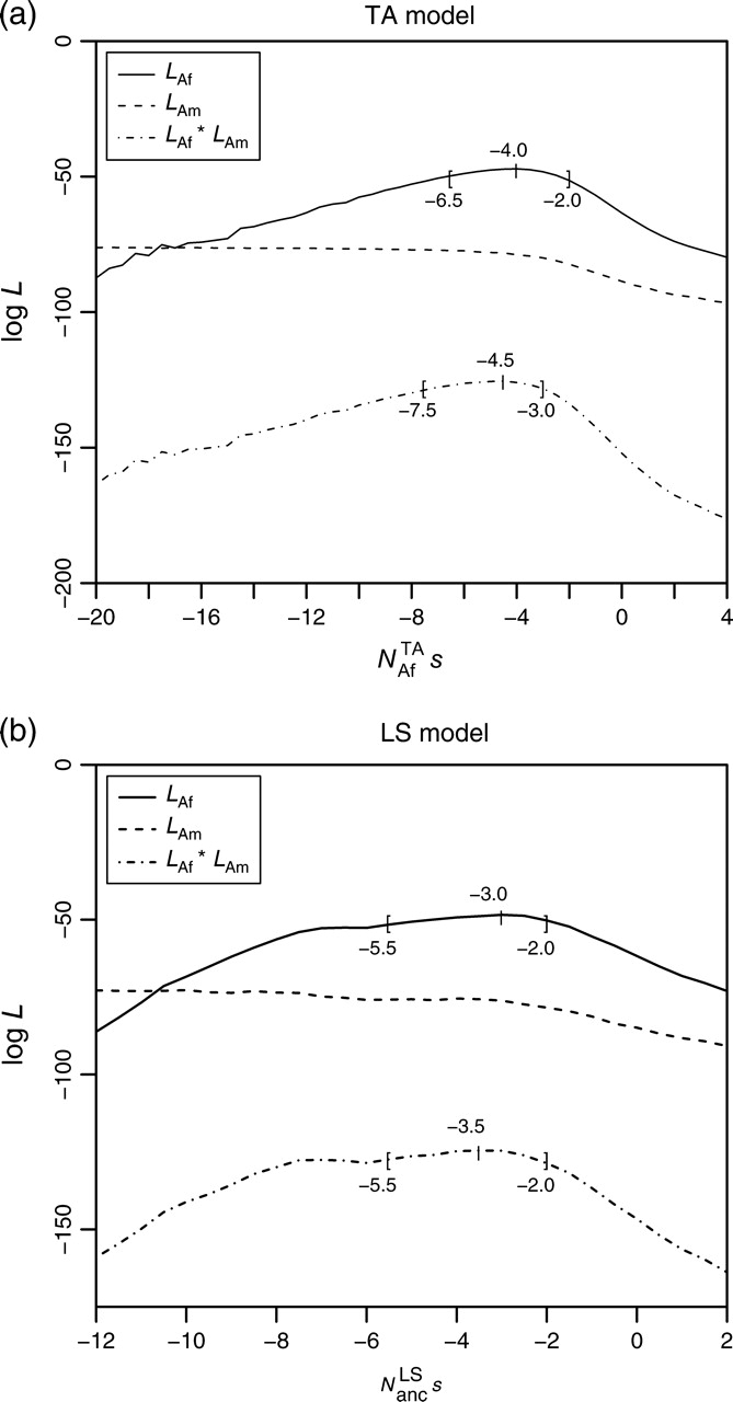
Likelihood curves for Ns based on BS element frequency data for North American, African, and combined Drosophila melanogaster subpopulations. On each curve, the ML estimate Ns* is indicated, as are the 2.5% and 97.5% confidence intervals. For North American data, no clear peaks in the likelihood curves can be observed and therefore no meaningful values Ns* and confidence intervals could be derived.

For the TA model, we estimate N_Af^TAs* = − 4.0 ( − 6.5,  − 2.0) for the likelihood L_Af^TA in the African subpopulation, and N_Af^TAs*  = −  4.5 ( − 7.5,  − 3.0) for the combined likelihood of the two subpopulations, L^TA = L_Af^TA×L_Am^TA. Both curves have clear peaks. In contrast, the likelihood curve L_Am^TA for the North American subpopulation alone is relatively flat. This implies that there is little information about the strength of selection at the time of emigration available from present-day North American frequencies, and also explains why L_Af^LS and L_Af^LS × L_Am^LS look qualitatively similar. The slightly lower ML estimate of the combined likelihood reflects the weak inclination of L_Am^LS toward more negative Ns values.

We also checked that—as expected due the loss of correlation between allele frequencies prior to and after the bottleneck—the unfactorized likelihood curve for the combined data of both subpopulations resembles the product L^TA of the individual likelihoods (data not shown). Unfactorized likelihoods were calculated according to equations (7) and (8). The required two-dimensional distributions ϕ(x_Am, x_Af) were numerically estimated by binning African and North American frequency pairs (x_Am, x_Af) from our simulations into grids of 10 × 10 bins, which keeps the overall number of bins comparable with that used for the individual one-dimensional distributions ϕ_Am and ϕ_Af. Our analysis further indicates that ML estimates are not sensitive to the particular choice of s in the American subpopulation after emigration. We obtain the same estimates for the African subpopulation and the combined subpopulations irrespective of whether s is set to zero in step 2 of our simulation algorithm or whether it remains at its ancestral value prior to the emigration from Africa (data not shown).

In the LS model, we again observe clear peaks in the likelihood curves for African data alone and combined data of both subpopulations, whereas North American data remain uninformative. ML estimates are N_anc^LSs*  = − 3.0 ( − 5.5,  − 2.0) for the African subpopulation, and N_anc^LSs*  = − 3.5 ( − 5.5,  − 2.0) for the combined subpopulations. Unfactorized likelihoods are also similar to the products of the individual likelihoods (data not shown).

Comparison of ML Estimates between Demographic Models

Our ML analysis yields informative point estimates for Ns* in the ancestral population for both demographic models, raising the question of how the respective estimates relate to each other. Notice that we measure strength of selection in units of N_anc^LSs for the LS model, using ancient African population size prior to the population expansion as the scaling factor. Our ML estimate N_anc^LSs*  = −  3.0 therefore implies that TEs in Africa evolve with Ns = −15 from the ancient population expansion on, as a result of the 5-fold increase in N while s is kept constant. At first glance, it might not seem obvious why a less-negative ML estimate is not observed for the LS model to conform to the estimated Ns = −4 of the TA model. However, as will be demonstrated in the following, the two ML estimates are indeed consistent with each other.

TE frequencies are assumed to be at transposition–selection equilibrium in the LS model prior to the ancient population expansion. According to our ML estimate, this equilibrium was specified by Ns = −3. The distribution of TE frequencies does not change during the population expansion and is therefore highly skewed toward high-frequency alleles compared with its destined new equilibrium for Ns = −15 after the expansion. Relaxation to this new equilibrium will occur over time and is driven by two mechanisms. First, TEs that transpose after the expansion evolve with Ns = −15. In the long run, their frequency distribution will therefore converge to the new transposition–selection equilibrium. TEs already present prior to the expansion, on the other hand, will continuously become lost from the population. Yet, among the accepted sites in our analysis, that is, those sites that were not lost during the bottleneck in North America and ascertained, ancient TEs clearly outnumbered newly transposed TEs. At N_anc^LSs  = − 3 we observe 77% of accepted TEs to be ancient. When assuming neutral evolution, the ratio increases to 93%. The reason for this is that at the time of emigration, there are still many more ancient TEs at higher frequencies compared with newly transposed TEs, and high-frequency alleles are less likely to become lost during the bottleneck. Although as a consequence of their negative selection coefficients, ancient TEs prevalently evolve toward lower frequencies since the expansion, this occurs relatively slowly. The average deterministic change of an allele's frequency x due to selection alone is described by the logistic equation dx/dt = (s/2)x(1 − x). Its solution is given by x(t) = (1 + [1/x(t₀) − 1] exp [s(t₀ − t)/2])⁻¹. The logistic equation is time symmetric. By rearranging its solution, we can thus express past frequencies x(t₀) as a function of present-day frequencies x_Af in the African subpopulation (notice also that time is measured in the direction from the present to the past in our two demographic models). For frequencies x_e at the time t_e of the population expansion, we obtain

(11)

From our ML estimate N_anc^LSs*  = − 3, we evaluate t_es ≈ 1.1. Each individual TE is of course also subject to random genetic drift, but averaged over a large ensemble of TEs the net effect of drift will be close to zero. The change in the frequency distribution of ancient TEs over time should thus be primarily governed by the deterministic shift due to selection. If at the time of population expansion, the frequency distribution was given by ρ(x, Ns) according to equation (2), that is, TEs were at transposition–selection equilibrium for the particular value of Ns, we expect to observe a distribution ρ(x_e[x_Af], Ns) at present. As can be seen in figure 4, we obtain ρ(x_e[x_Af], − 3) ≈ ρ(x, −4) for our ML estimate of the LS model. Consequently, the present-day frequency distribution of ancient TEs will essentially resemble that of a constant-sized panmictic population evolving at Ns = −4, in full accordance with the ML estimate obtained from the TA model.

FIG. 4.—

Expected present-day frequency distributions of ancient TEs if only the deterministic effect of selection is taken into account. The expected present-day densities at frequencies x_Af are given by the equilibrium density distributions (2) at positions x_e[x_Af] using equation (11). The solid black line specifies transposition–selection equilibrium ρ(x_Af, − 4) for a panmictic population of constant size, corresponding to the ML estimate of the TA model.

Goodness of Fit of Our ML Estimates

Our ML framework allowed us to identify the most likely estimate Ns* for our frequency data, given a particular demographic model. To check whether the observed data are in fact compatible with the model, we performed two-sided Kolmogorov–Smirnov (KS) goodness of fit tests between the distributions of measured BS frequencies and the expected distributions obtained from our simulations. Significance values for calculated KS D-values were empirically determined by resampling from the simulated reference distribution. In each resampling step, 18 frequencies x_i were randomly drawn from the reference distribution. For every frequency x_i, a random number k_i was then drawn from a binomial distribution B_xi(k_i | n_i = 40), specifying the number of individuals that carry the allele in a sample of size 40. The yielded set of 18 frequencies {k_i/40} defines one sample. For a given KS test statistic D*, the corresponding P value was then calculated by estimating Pr(D ≥ D*) from 10⁵ generated samples.

KS goodness of fit tests applied to the observed cumulative frequency distribution of BS elements in the African subpopulation yield D = 0.20 (P = 0.44) for the TA model and D = 0.25 (P = 0.39) for the LS model at their respective ML estimates Ns*. The null hypothesis that observed frequencies are drawn from the simulated distributions can hence be accepted for both demographic scenarios. For North American data, in contrast, we obtain D = 0.62 (P < 10⁻⁵) for the TA model and D = 0.56 (P < 10⁻⁵) for the LS model. The null hypothesis can clearly be rejected in both cases. The main reason for the poor fit of North American data can be recognized in figure 5, where observed and expected cumulative frequency distributions are shown for the two demographic models at their respective ML estimates. Although observed and expected distributions fit well for African data, a large discrepancy exists in North American data between the approximately 30% of elements predicted to have become fixed and the complete lack of such fixed elements in our data. The likelihood of observing no fixed element in a set of 18 tested elements is only 0.0016 assuming an individual fixation probability of 0.3.

FIG. 5.—

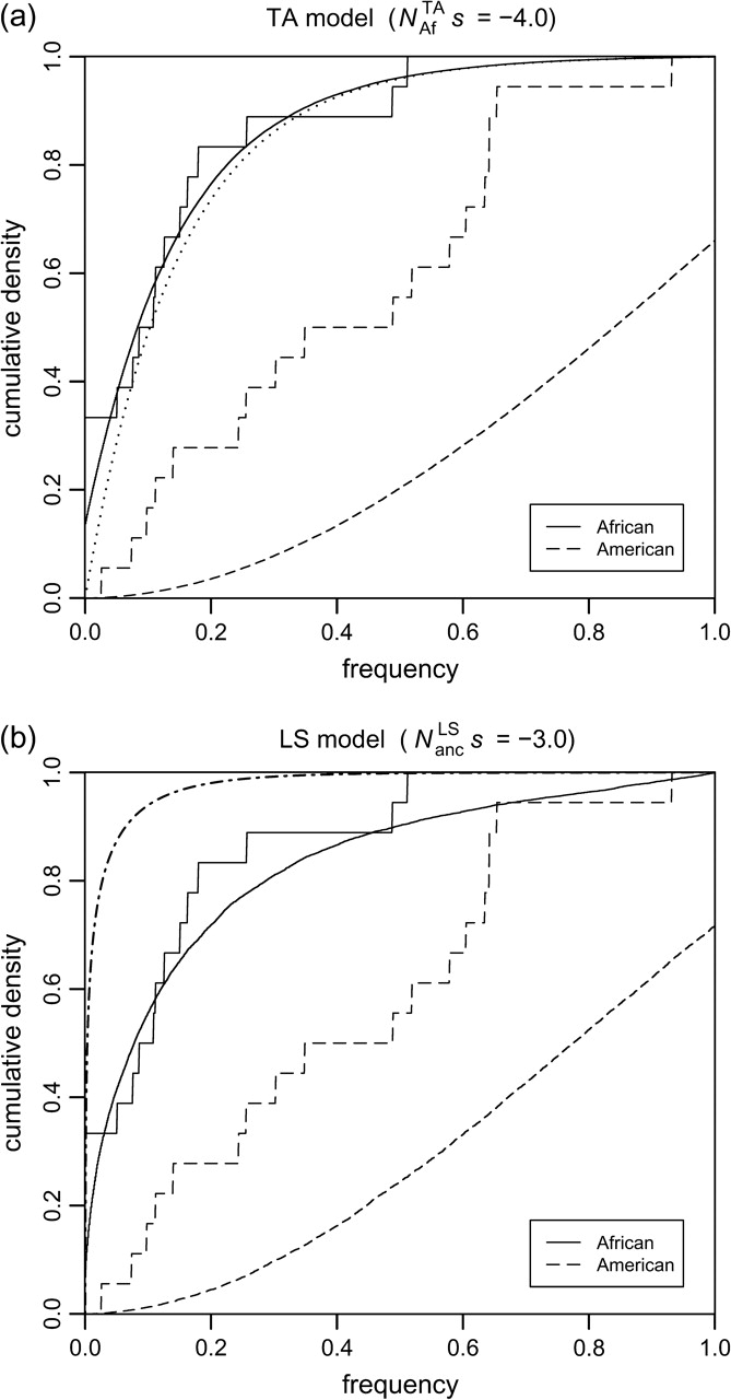
Cumulative distributions of observed (step functions) and expected (continuous curves) frequencies of BS elements for both demographic models at their respective ML estimates. The dotted line in (a) shows the normalized distribution ∫₀^xyρ(y, − 4) dy, which corresponds well with the expected distribution of African BS frequencies for the TA model. The dash-dotted line in (b) is the theoretical transposition–selection equilibrium distribution ∫₀^xρ(y, − 4) dy.

Excluding fixed North American elements from the simulated distributions improves the goodness of fit, but P values remain below a significance level of 1% (LS: P < 0.002, TA: P < 0.001). In any case, this exclusion would be hard to justify. The expected ratio of fixed TEs is an intrinsic property of both demographic models given the strength of their bottleneck parameters. There is also no evident bias toward polymorphic TEs when choosing the BS elements that constitute our experimental data set. Along another line of thought one could assume that, for some reason, selection prevents TEs from ultimately becoming fixed during the bottleneck. But such a mechanism is hard to argue for too, considering the substantial reduction of effective population size during the bottleneck, which profoundly diminishes effectiveness of all types of selection. So far, the reason for why we do not observe more fixed TEs in North America remains obscure, but presumably the bottleneck scenario for D. melanogaster demography has to be refined, possibly by allowing for the existence of gene flow beyond that assumed in a single severe bottleneck scenario.

ML Estimates for a Constant-Sized Panmictic Population

Our ML estimates can be compared with those obtained when using the method of Petrov et al. (2003). In this method, only one constant-sized panmictic population at transposition–selection equilibrium is assumed without taking into account particular population substructure. Ascertainment bias resulting from the fact that BS elements were initially identified in only one sequenced strain is incorporated analogously to our method. The probability of observing an element at frequency x is hence given by the (normalized) posterior probability density function Pr(x, Ns) ∝ x × ρ (x, Ns) for both African and North American data.

If the method of Petrov et al. (2003) is applied to our BS frequency data, we obtain a ML estimate Ns* = −2.3 (−3.4, −1.3) for the combined set where element sample frequencies of all North American and African strains are pooled together to assume one single panmictic population. Disregarding bottleneck and population substructure thus leads to a considerably weaker inferred selection intensity. In contrast to our method, one also observes a clear peak for the likelihood curve of North American data alone yielding an estimate Ns* = −1.0 (−2.3, 0.9) that overlaps with neutral evolution. This, however, can clearly be rejected by our analysis. For African data alone, on the other hand, we obtain Ns* = −4.6 (−7.3, −2.7) in close agreement with our result. The divergent point estimate of both methods for the combined data therefore presumably owes to the different North American estimates.

Effects of a Bottleneck on the Ancestral Frequency Distribution

The observation of coinciding estimates for African data between our method and the one of Petrov et al. (2003) is instructive in understanding the effects that ascertainment in a derived population has on the observed allele frequency distribution in the ancestral population. After all, in the approach of Petrov et al. (2003) bottleneck effects are ignored completely. Furthermore, Petrov et al. (2003) explicitly incorporate ascertainment bias for the entire population, whereas in our method ascertainment is only performed in North America.

Due to the lack of correlation between allele frequencies prior to and after the bottleneck, ascertainment has only negligible effect on the distribution of African TE frequencies in our analysis. For example, we obtain the same Ns* = −4.0 for the TA model, irrespective of whether we incorporate ascertainment bias for North American TE frequencies, or not (data not shown). Hence, the effect of ascertainment on the frequency distribution in Africa is expected to be far more profound in the method of Petrov et al. (2003) compared with our method.

That despite these essential differences both methods yield similar results is the consequence of a fundamental similarity between the effects of intense population bottlenecks and ascertainment in a single strain. This similarity arises from the fact that the probability of an allele to not become lost during a strong bottleneck is approximately proportional to its initial frequency x. The functional effects of a severe bottleneck on the ancestral allele frequency distribution hence closely resemble those of ascertainment in a single strain. As can be seen in figure 5, the expected distribution of African BS frequencies derived from our simulations indeed fits well to the theoretical approximation x × ρ (x, Ns*), which coincides with the analytic form used by Petrov et al. (2003), although in their approach the proportionality to x arose from ascertainment and not from the bottleneck.

A convenient implication of this finding is that selection strength can be reliably inferred from ancestral populations if the bottleneck was severe enough to effectively uncouple allele frequencies between ancestral and derived populations. In this case, the expected frequency distribution for ancestral data becomes independent of the particular ascertainment scheme used in the derived population and the exact bottleneck parameters. Assuming transposition–selection equilibrium, the expected ancestral frequency distribution can then be well approximated by the normalized distribution x × ρ (x, Ns). This heuristic approach is of course only applicable to TEs that were already present prior to the emigration and thus cannot be used for TE families that experienced strong purifying selection in the derived population. In our analysis, the information present in the African sample sufficed to yield relatively narrow confidence intervals surrounding our point estimate of Ns = −4 in Africa, which is consistent with the general observation that TEs are under purifying selection in Drosophila (Charlesworth and Langley 1989).

If, however, the bottleneck was only moderate, neither of the above two approximations might hold to a sufficient extent. First, allele frequencies might still be substantially correlated between the ancestral and emigrated subpopulations, in which case the ancestral frequency distribution will also be affected by ascertainment performed in the emigrated subpopulation. And second, the probability of not becoming fixed during the bottleneck will show a more complex functional dependence on the allele's initial frequency. In such cases, our method still provides an adequate framework to model the expected frequency distributions in ancestral and emigrated subpopulations and infer from it ML estimates of selection intensity in the ancestral population.

In contrast to ancestral frequency data, our analysis suggests that there is generally very little information about the strength of ancestral purifying selection present in frequency data from the derived population due to the loss of correlation between ancestral and present-day allele frequencies during the bottleneck. Selection coefficients inferred from non-African frequency data under the assumption of constant population size should therefore be recalculated, as suggested by the inconsistent results between our method and the method of Petrov et al. (2003) for such data. For D. melanogaster in particular, the situation is further complicated by the uncertainty surrounding the bottleneck parameters. We investigated the two bottleneck scenarios from Thornton and Andolfatto (2006) and Li and Stephan (2006) and did not find the predicted results for the frequency distribution in North America to be fully compatible with the one observed among BS elements from our experimental data set. A possible reason for this discrepancy could be that the bottleneck was actually less intense than assumed by the two investigated demographic models. There is indeed additional reason to suspect that bottleneck estimates from the two scenarios are too intense, because the data used to produce these estimates come exclusively from the X chromosome (Glinka et al. 2003; Haddrill et al. 2005), where reduction in neutral polymorphism due to adaptive substitution may be more prevalent than on the autosomes (Singh et al. 2007) (but see also Thornton et al. 2006). If the bottleneck were less intense, then the loss of frequency correlation during the bottleneck would also be less severe, and we would thus have more information with which to infer the ancestral selection coefficient from the North American population.

Extendability of Our Method

We investigated the demographic scenarios for D. melanogaster from Thornton and Andolfatto (2006) and Li and Stephan (2006), but our ML approach can be applied to other demographic models and/or other species in a straightforward fashion. The two particular models examined in our analysis comprise key features such as emigration, bottleneck, and population expansion, from which a large class of possible demographic scenarios can be constructed. The only requirement for our approach to be applicable is that the ancestral population can assumed to be in panmictic equilibrium at some defined moment in the past such that allele frequencies were in transposition–selection equilibrium then. It has to be taken into account, however, that for scenarios with very ancient population expansions the algorithm becomes less efficient due to the necessity of simulating large numbers of new transposition events. Different ascertainment schemes can be easily incorporated into our methodology as well.

A crucial specification of our model is also the particular type of selection used. We assumed that TEs have a codominant fitness effect in heterozygotes. There is some debate in the literature about the characteristic dominance of TEs; fitness effects due to gene disruptions by TE insertions would be expected to be dominant or codominant, whereas fitness effects due to ectopic recombination among dispersed TE copies would be expected to be underdominant (Montgomery et al. 1991; Petrov et al. 2003). Empirical work suggests that the fitness effects of TEs from the copia family in D. melanogaster are codominant (Fry and Nuzhdin, 2003). If selection against other families were underdominant, though, this could change our results. Underdominance shifts the frequency distribution to lower frequencies for a given Ns, so we would expect the point estimate and confidence intervals for Ns to shift toward positive values. Petrov et al. (2003) did explore the effects of underdominance and full dominance on inference of Ns and found their conclusions to be qualitatively unchanged. Different selection schemes than codominance are straightforward to implement in our analysis, as long as the distribution of allele frequencies in transposition–selection equilibrium is known for the particular type of selection used. The binomial sampling procedure used to generate TE trajectories in our simulations must then be modified accordingly.

Implications for Ancestral TE Copy Number

The number of copies of a TE per genome is a key indicator of its rate of transposition and the strength of selection acting against it (Charlesworth and Langley 1989). When the population experiences a bottleneck, the copy number can decrease for this reason alone. Further, there is some evidence to suggest that the colonization event following the bottleneck event may have increased the rate of transposition in Drosophila (Vieira et al. 2002; Nardon et al. 2005). Thus, it is important to understand the effects of demography on copy number. In particular, we might wish to know whether copy number is expected to differ between North American and African populations and what effect purifying selection against the elements might have on this difference.

The expected copy numbers for the BS family at the time the bottleneck began and at present day in Africa can roughly be calculated, continuing with the assumptions made throughout the paper. We emphasize, however, that the following calculations have to be taken with a grain of salt as they rely partly on the simulated distribution of TE frequencies in the North American subpopulation, which we could not fit well to the experimentally observed distribution.

The expected number of BS elements per haploid genome in a North American fly is m × E[x_Am], where m is the number of unique insertion sites overall in the North American subpopulation and the expectation value E[x_Am] is estimated according to the BS element frequency distribution ϕ(x) in North America. From our simulations with Ns = −4 in the TA model, E[x_Am] is 0.55. Note that here ϕ(x) corresponds to the distribution of BS element frequencies without the ascertainment step performed; the mean element frequency of the distribution with ascertainment performed is 0.75. Based on 29 BS elements in version 3 of the D. melanogaster reference sequence, we would estimate there to be m = 53 insertion sites in the North American population.

The fraction of polymorphisms lost during the bottleneck, according to our simulations with Ns = −4 in the TA model, was 97.9%. Thus, if 53 sites remain, there were approximately 2,500 insertion sites at the beginning of the bottleneck. If the population was at equilibrium when the bottleneck began, as assumed for the TA model, then the expected number of BS elements per haploid genome at this time is just 2,500 × E[x_Af]. We find E[x_Af] to be 0.012 by numerical integration of x × ρ(x, Ns = −4), which implies there to be about 30 elements in a given ancestral haploid genome; if the African subpopulation persists at transposition–selection balance to the present day, then we would also expect 30 elements per contemporary haploid African genome. Analogous calculations with Ns = 0 rather than Ns = −4 imply about 440 insertion sites in the ancestral population. Because the mean frequency under neutrality, 0.067, is considerably larger than the 0.012 for Ns = −4, we would expect about 29 elements per ancestral or contemporary African, haploid genome.

These illustrative calculations suggest that the copy number per genome is actually expected to be similar in North American and African populations and that it will be difficult to infer the strength of purifying selection based on copy number per genome, because the expected modern African copy number will not differ significantly under purifying selection and neutrality. They also suggest that, if one were to screen a sample from an African population for the presence of TEs, the stronger the purifying selection against an element, the more insertion sites one expects, and the fewer elements per insertion site.

We can also apply the above approach to derive the expected number of heterozygous sites in a diploid individual, which is given by m × E[2x(1 − x)]. Using our ML estimate Ns = −4 of the TA model, we estimate to observe on average 53 × E[2x_Am(1 − x_Am)] ≈ 14 heterozygous sites per individual in the North American population. This number is considerably larger in African individuals, where we obtain 2,500 × E[2x_Af(1 − x_Af)] ≈ 50. The intensity of purifying selection against individual elements should hence be much lower in the derived population due to the lower probability of ectopic recombination between dispersed heterozygous elements. This retrospectively justifies our approximation of s = 0 in the North American population.

Transposition–Selection Balance

One question of much interest in the study of TEs concerns heterogeneity in the rate of transposition in time. Transposition might proceed at an essentially constant rate, with growth in element numbers checked by a constant rate of loss due to excision and purifying selection (Charlesworth and Langley 1989). However, an alternative hypothesis for which there is some experimental support holds that transposition rates might vary substantially in time if transposition–selection balance occurs as a coevolutionary arms race between TEs and repressors of transposition (Nuzhdin et al. 1998). Under this hypothesis, a mutation that allowed TEs to multiply at great rates would yield a burst of transposition in a population, until a second mutation restricting the rate of transposition appears. If we were to examine the frequency distribution under the former hypothesis, we would expect to infer the presence of purifying selection. Under the latter hypothesis, assuming that we sample from the population outside a period of rapid transposition, we would expect to observe elements segregating neutrally.

Petrov et al. (2003) speculated that the hypothesis of coevolutionary cycles in transposition rate might be supported by their estimates of Ns, which overlapped with zero for two of the four TE families they studied, including the BS family. In this study, incorporation of a demographic model results in a confidence interval for Ns that does not overlap with 0, and thus we are able to reject the hypothesis that Ns = 0 within the assumptions of our model. Frequency data from many more families would be required to answer this question more conclusively, but so far as our analysis bears on the question, the BS element frequencies are not consistent with the hypothesis that they are segregating neutrally in Africa, and thus there is no evidence to reject the hypothesis that the family exists in transposition–selection balance.

Implications for the Inference of Selection in a Demographic Context

A recent bottleneck is a common demographic pattern in several species of evolutionary genetic interest, including D. melanogaster (Li and Stephan 2006; Thornton and Andolfatto 2006), maize (Wright et al. 2005), and human (Harpending et al. 1998). Our results bear on studies designed to infer the intensity of selection on genetic variation from frequency data in such populations, which we anticipate will become more numerous as large population genomic data sets become available. Our study underscores the importance of accounting for demography for such inference, as has been pointed out in numerous other contexts (e.g., Andolfatto and Przeworski 2001; Teshima et al. 2006; Thornton and Jensen 2007; Innan and Kim 2008; Macpherson et al. 2008).

An alternative method that estimates Ns based on comparison between polymorphism and divergence exists (Bustamante et al. 2002, 2005), and this method has been shown to be relatively robust to nonconstant demographic patterns. However, this method does not use the frequency of polymorphisms to obtain its estimates, which we have shown to be informative about the strength of selection, and further assumes that the strength of selection has remained constant from the time of divergence to the present. Thus, the two methods of inference use complementary information, and, where satisfactory demographic models exist for a population, comparison between their results should prove instructive.

Our analysis suggests that frequency data from a derived population carry little information about the strength of selection in the ancestral population compared with ancestral frequency data itself. This discrepancy arises from the fact that a severe bottleneck can effectively diminish correlation between an allele's frequency in the ancestral population and that in the derived population. The effect of the bottleneck on the expected ancestral frequency distribution is then determined by the probability of an allele to not become lost during the bottleneck, which is roughly proportional to its initial frequency at emigration.

As a consequence, for a severe enough bottleneck, the expected frequency distribution in the ancestral population can be well approximated by a simple heuristic approach, where the actual frequency distribution in the population is multiplied by the allele frequency x. The effect of an intense bottleneck can therefore be thought of as performing ascertainment in a single strain from the ancestral population.

However, in many realistic demographic scenarios, bottlenecks might not be severe enough for the heuristic approach to apply adequately. In addition, the ancestral allele frequency distribution will often be far from transposition–selection equilibrium, for example, if the demography features an ancient population expansion. Results derived from the simple heuristic approach can be substantially misleading in such cases. For example, when applying the demographic model of Li and Stephan (2006) to our BS data from D. melanogaster, we obtained a widely divergent estimate of Ns = −15 for the strength of selection against BS elements in the present-day African population compared with Ns = −4 obtained when using the simpler demographic scenario of Thornton and Andolfatto (2006), although both estimates correspond to similar ancestral allele frequency distributions at emigration within their respective models.

For many realistic demographic scenarios, the particular demographic history will thus have a profound effect on the inferred ancestral selection intensity if ascertainment has been performed in a derived population that encountered a population bottleneck after emigration. Our ML approach provides a flexible methodology for such cases that allows for a reliable inference of ancestral selection intensity among a broad class of possible demographic models and ascertainment schemes. Its application should therefore improve our understanding of the characteristic mode of selection for species with complicated demographic histories.

Supplementary Material

Supplementary tables S1 and S2 are available at Molecular Biology and Evolution online (http://www.mbe.oxfordjournals.org/).

References

- Andolfatto P, Przeworski M. Regions of lower crossing over harbor more rare variants in African populations of Drosophila melanogaster. Genetics. 2001;158:657–665. doi: 10.1093/genetics/158.2.657. [DOI] [PMC free article] [PubMed] [Google Scholar]
- Biemont C, Vieira C. Genetics: junk DNA as an evolutionary force. Nature. 2006;443:521–524. doi: 10.1038/443521a. [DOI] [PubMed] [Google Scholar]
- Bustamante CD, Fledel-Alon A, Williamson S, et al. (14 co-authors) Natural selection on protein-coding genes in the human genome. Nature. 2005;437:1153–1157. doi: 10.1038/nature04240. [DOI] [PubMed] [Google Scholar]
- Bustamante CD, Nielsen R, Sawyer SA, Olsen KM, Purugganan MD, Hartl DL. The cost of inbreeding in Arabidopsis. Nature. 2002;416:531–534. doi: 10.1038/416531a. [DOI] [PubMed] [Google Scholar]
- Casacuberta E, Pardue ML. Coevolution of the telomeric retrotransposons across Drosophila species. Genetics. 2002;161:1113–1124. doi: 10.1093/genetics/161.3.1113. [DOI] [PMC free article] [PubMed] [Google Scholar]
- Charlesworth B, Langley CH. The population genetics of Drosophila transposable elements. Annu Rev Genet. 1989;23:251–287. doi: 10.1146/annurev.ge.23.120189.001343. [DOI] [PubMed] [Google Scholar]
- Charlesworth B, Sniegowski P, Stephan W. The evolutionary dynamics of repetitive DNA in eukaryotes. Nature. 1994;371:215–220. doi: 10.1038/371215a0. [DOI] [PubMed] [Google Scholar]
- Ewens WJ. Mathematical population genetics. 2nd ed. New York: Springer; 2004. [Google Scholar]
- Fry JD, Nuzhdin SV. Dominance of mutations affecting viability in Drosophila melanogaster. Genetics. 2003;163:1357–1364. doi: 10.1093/genetics/163.4.1357. [DOI] [PMC free article] [PubMed] [Google Scholar]
- Glinka S, Ometto L, Mousset S, Stephan W, De Lorenzo D. Demography and natural selection have shaped genetic variation in Drosophila melanogaster: a multi-locus approach. Genetics. 2003;165:1269–1278. doi: 10.1093/genetics/165.3.1269. [DOI] [PMC free article] [PubMed] [Google Scholar]
- Haddrill PR, Thornton KR, Charlesworth B, Andolfatto P. Multilocus patterns of nucleotide variability and the demographic and selection history of Drosophila melanogaster populations. Genome Res. 2005;15:790–799. doi: 10.1101/gr.3541005. [DOI] [PMC free article] [PubMed] [Google Scholar]
- Harpending HC, Batzer MA, Gurven M, Jorde LB, Rogers AR, Sherry ST. Genetic traces of ancient demography. Proc Natl Acad Sci USA. 1998;95:1961–1967. doi: 10.1073/pnas.95.4.1961. [DOI] [PMC free article] [PubMed] [Google Scholar]
- Hua-Van A, Rouzic AL, Maisonhaute C, Capy P. Abundance, distribution and dynamics of retrotransposable elements and transposons: similarities and differences. Cytogenet Genome Res. 2005;110:426–440. doi: 10.1159/000084975. [DOI] [PubMed] [Google Scholar]
- Innan H, Kim Y. Detecting local adaptation using the joint sampling of polymorphism data in the parental and derived populations. Genetics. 2008;179:1713–1720. doi: 10.1534/genetics.108.086835. [DOI] [PMC free article] [PubMed] [Google Scholar]
- Kaminker JS, Bergman CM, Kronmiller B, et al. (12 co-authors) The transposable elements of the Drosophila melanogaster euchromatin: a genomics perspective. Genome Biol. 2002 doi: 10.1186/gb-2002-3-12-research0084. 3:RESEARCH0084. [DOI] [PMC free article] [PubMed] [Google Scholar]
- Kazazian HH. Mobile elements: drivers of genome evolution. Science. 2004;303:1626–1632. doi: 10.1126/science.1089670. [DOI] [PubMed] [Google Scholar]
- Knuth DE. 3rd ed. Reading (MA):: Addison-Wesley Professional; 1997. Art of computer programming. Vol. 2: Seminumerical algorithms. [Google Scholar]
- Li H, Stephan W. Inferring the demographic history and rate of adaptive substitution in Drosophila. PLoS Genet. 2006;2:e166. doi: 10.1371/journal.pgen.0020166. [DOI] [PMC free article] [PubMed] [Google Scholar]
- Lipatov M, Lenkov K, Petrov DA, Bergman CM. Paucity of chimeric gene-transposable element transcripts in the Drosophila melanogaster genome. BMC Biol. 2005;3:24–24. doi: 10.1186/1741-7007-3-24. [DOI] [PMC free article] [PubMed] [Google Scholar]
- Macpherson JM, Gonzalez J, Witten DM, Davis JC, Rosenberg NA, Hirsh AE, Petrov DA. Nonadaptive explanations for signatures of partial selective sweeps in Drosophila. Mol Biol Evol. 2008;25:1025–1042. doi: 10.1093/molbev/msn007. [DOI] [PMC free article] [PubMed] [Google Scholar]
- McDonald JF, Matyunina LV, Wilson S, Jordan IK, Bowen NJ, Miller WJ. LTR retrotransposons and the evolution of eukaryotic enhancers. Genetica. 1997;100:3–13. [PubMed] [Google Scholar]
- Medstrand P, van de Lagemaat LN, Dunn CA, Landry JR, Svenback D, Mager DL. Impact of transposable elements on the evolution of mammalian gene regulation. Cytogenet Genome Res. 2005;110:342–352. doi: 10.1159/000084966. [DOI] [PubMed] [Google Scholar]
- Montgomery E, Charlesworth B, Langley CH. A test for the role of natural selection in the stabilization of transposable element copy number in a population of Drosophila melanogaster. Genet Res. 1987;49:31–41. doi: 10.1017/s0016672300026707. [DOI] [PubMed] [Google Scholar]
- Montgomery EA, Huang SM, Langley CH, Judd BH. Chromosome rearrangement by ectopic recombination in Drosophila melanogaster: genome structure and evolution. Genetics. 1991;129:1085–1098. doi: 10.1093/genetics/129.4.1085. [DOI] [PMC free article] [PubMed] [Google Scholar]
- Moran JV, DeBerardinis RJ, Kazazian HH. Exon shuffling by L1 retrotransposition. Science. 1999;283:1530–1534. doi: 10.1126/science.283.5407.1530. [DOI] [PubMed] [Google Scholar]
- Nagylaki T. The moments of stochastic integrals and the distribution of sojourn times. Proc Natl Acad Sci USA. 1974;71:746–749. doi: 10.1073/pnas.71.3.746. [DOI] [PMC free article] [PubMed] [Google Scholar]
- Nardon C, Deceliere G, Loevenbruck C, Weiss M, Vieira C, Biémont C. Is genome size influenced by colonization of new environments in dipteran species? Mol Ecol. 2005;14:869–878. doi: 10.1111/j.1365-294X.2005.02457.x. [DOI] [PubMed] [Google Scholar]
- Nuzhdin SV. Sure facts, speculations, and open questions about the evolution of transposable element copy number. Genetica. 1999;107:129–137. [PubMed] [Google Scholar]
- Nuzhdin SV, Pasyukova EG, Morozova EA, Flavell AJ. Quantitative genetic analysis of copia retrotransposon activity in inbred Drosophila melanogaster lines. Genetics. 1998;150:755–766. doi: 10.1093/genetics/150.2.755. [DOI] [PMC free article] [PubMed] [Google Scholar]
- Petrov DA, Aminetzach YT, Davis JC, Bensasson D, Hirsh AE. Size matters: non-LTR retrotransposable elements and ectopic recombination in Drosophila. Mol Biol Evol. 2003;20:880–892. doi: 10.1093/molbev/msg102. [DOI] [PubMed] [Google Scholar]
- Sawyer S, Hartl D. Population genetics of polymorphism and divergence. Genetics. 1992;132:1161–1176. doi: 10.1093/genetics/132.4.1161. [DOI] [PMC free article] [PubMed] [Google Scholar]
- Singh N, Macpherson JM, Jensen J, Petrov D. Similar levels of X-linked and autosomal nucleotide variation in African and non-African populations of Drosophila melanogaster. BMC Evol Biol. 2007;7:202. doi: 10.1186/1471-2148-7-202. [DOI] [PMC free article] [PubMed] [Google Scholar]
- Singh ND, Arndt PF, Petrov DA. Genomic heterogeneity of background substitutional patterns in Drosophila melanogaster. Genetics. 2005;169:709–722. doi: 10.1534/genetics.104.032250. [DOI] [PMC free article] [PubMed] [Google Scholar]
- Teshima KM, Coop G, Przeworski M. How reliable are empirical genomic scans for selective sweeps? Genome Res. 2006;16:702–712. doi: 10.1101/gr.5105206. [DOI] [PMC free article] [PubMed] [Google Scholar]
- Thornton K, Andolfatto P. Approximate Bayesian inference reveals evidence for a recent, severe bottleneck in a Netherlands population of Drosophila melanogaster. Genetics. 2006;172:1607–1619. doi: 10.1534/genetics.105.048223. [DOI] [PMC free article] [PubMed] [Google Scholar]
- Thornton K, Bachtrog D, Andolfatto P. X chromosomes and autosomes evolve at similar rates in Drosophila: no evidence for faster-X protein evolution. Genome Res. 2006;16:498–504. doi: 10.1101/gr.4447906. [DOI] [PMC free article] [PubMed] [Google Scholar]
- Thornton KR, Jensen JD. Controlling the false-positive rate in multilocus genome scans for selection. Genetics. 2007;175:737–750. doi: 10.1534/genetics.106.064642. [DOI] [PMC free article] [PubMed] [Google Scholar]
- Vieira C, Nardon C, Arpin C, Lepetit D, Biémont C. Evolution of genome size in Drosophila: is the invader's genome being invaded by transposable elements? Mol Biol Evol. 2002;19:1154–1161. doi: 10.1093/oxfordjournals.molbev.a004173. [DOI] [PubMed] [Google Scholar]
- Volff JN. Turning junk into gold: domestication of transposable elements and the creation of new genes in eukaryotes. Bioessays. 2006;28:913–922. doi: 10.1002/bies.20452. [DOI] [PubMed] [Google Scholar]
- Wright SI, Bi IV, Schroeder SG, Yamasaki M, Doebley JF, McMullen MD, Gaut BS. The effects of artificial selection on the maize genome. Science. 2005;308:1310–1314. doi: 10.1126/science.1107891. [DOI] [PubMed] [Google Scholar]
Associated Data
This section collects any data citations, data availability statements, or supplementary materials included in this article.