

Abstract
Many physiological responses elicited by neuronal spikes—intracellular calcium transients, synaptic potentials, muscle contractions—are built up of discrete, elementary responses to each spike. However, the spikes occur in trains of arbitrary temporal complexity, and each elementary response not only sums with previous ones, but can itself be modified by the previous history of the activity. A basic goal in system identification is to characterize the spike-response transform in terms of a small number of functions—the elementary response kernel and additional kernels or functions that describe the dependence on previous history—that will predict the response to any arbitrary spike train. Here we do this by developing further and generalizing the “synaptic decoding” approach of Sen et al. (J Neurosci 16:6307-6318, 1996). Given the spike times in a train and the observed overall response, we use least-squares minimization to construct the best estimated response and at the same time best estimates of the elementary response kernel and the other functions that characterize the spike-response transform. We avoid the need for any specific initial assumptions about these functions by using techniques of mathematical analysis and linear algebra that allow us to solve simultaneously for all of the numerical function values treated as independent parameters. The functions are such that they may be interpreted mechanistically. We examine the performance of the method as applied to synthetic data. We then use the method to decode real synaptic and muscle contraction transforms.
Keywords: Motor control, spike trains, synaptic transmission, synaptic plasticity, neuromuscular, nonlinear system identification, neurophysiological input-output transform, mathematical modeling
Introduction
The spike is a basic organizing unit of neural activity. Each discrete spike stimulus elicits a discrete elementary response that propagates through various neurophysiological pathways. The prototypical example is at the synapse, where each presynaptic spike elicits, in turn, a discrete rise in presynaptic calcium concentration, release of neurotransmitter, and changes in postsynaptic conductance, current, and potential (Katz 1969; Johnston and Wu, 1995; Sabatini and Regehr, 1999). The fundamental difficulty in understanding the stimulus-response relationship in such cases comes from the fact that the spikes occur in trains of arbitrary temporal complexity, and that each elementary response not only sums with previous ones, but can itself be greatly modified by the previous history of the activity—in synaptic physiology, by the well-known processes of synaptic plasticity such as facilitation, depression, and post-tetanic potentiation (Magleby and Zengel, 1975, 1982; Krausz and Friesen, 1977; Zengel and Magleby 1982; Sen et al., 1996; Hunter and Milton, 2001; Zucker and Regehr, 2002). Downstream of but implicitly including these processes of synaptic plasticity, when they occur at a neuromuscular junction, is then such a response as muscle contraction. In this paper we will analyze, in addition to synthetic data, experimental data from a “slow” invertebrate muscle where prolonged response summation and a highly nonlinear and plastic neuromuscular transform (Brezina et al., 2000) make for a very complex, irregular response that, at first sight, appears extremely challenging to understand and predict quantitatively. Fig. 1 illustrates some of the factors that are responsible for the complexity of the spike-response transform with synthetic data.
Fig. 1.

The problem dealt with in this paper: the complex spike-response transform and its decoding, illustrated with the model used in most of this paper and representative synthetic function forms. A: The forms assumed here for the three functions K, H, and F that, according to the model, build up the spike-response transform. B: The building up of the transform from the functions in panel A by the operation of the model, applying, from bottom to top, first Eq. 2 and then Eq. 1 in Methods. First, each spike of the spike train {ti} (blue dots along the bottom) elicits an instance of the dynamic kernel H that sums with previous instances (as indicated by the thin black curves of the bottom set of waveforms) to give the overall waveform Σi H (thick black curve). Σi H is then transformed by the static nonlinear function F to give the waveform A (dark blue curve). Each spike also elicits an instance of the dynamic kernel K (the elementary single-spike response kernel), which is scaled in amplitude by Ai, the value of A at that spike time (dark blue dots on A and arrows up to the top set of waveforms) and summed with previous instances (as indicated by the thin black curves of the top set of waveforms) to give the overall response R to the spike train (blue curve). Note how, due to the slow speed of K relative to the typical interspike interval, the instances of K summate and fuse, so that the shape of K cannot be discerned in R by simple inspection. Neither can K be seen in isolation simply by making the interspike intervals longer, because after an interspike interval that is longer than H, there is (with F(0) = 0) no response at all (e.g., at the two downward arrows). C: The goal of the decoding method is, given only {ti} and R, to extract functions K̂, Ĥ, and F̂ that are good estimates of the true functions K, H, and F.
To achieve a predictive understanding of the spike-response transform is our goal here. As indicated in Fig. 1, from the observable data, just the spike train and overall response to it, we wish to extract a set of building-block functions—the elementary response kernel and other functions that describe the dependence of the response on the previous history—that will allow us to predict quantitatively the response not only to that particular spike train, but to any arbitrary spike train. This will constitute a complete spike-level characterization of the spike-response transform.
The problem is one of nonlinear system identification. In neurophysiology, and synaptic physiology in particular, such problems have been approached by several methods (for a comparative overview see Marmarelis, 2004). A classic method is to fit the data with a specific model (e.g., Magleby and Zengel, 1975, 1982; Zengel and Magleby, 1982). However, the choice of model must typically be guided by the limited dataset itself, so that often the model fails to generalize. In a model-free approach, on the other hand, white-noise stimulation is used to determine the system's Volterra, Wiener, or other similar kernel expansion (e.g., Marmarelis and Naka, 1973; Krausz and Friesen, 1977; Gamble and DiCaprio, 2003; Song et al., 2009a,b; for reviews see Sakai, 1992; Marmarelis, 2004). Although in principle providing a complete, general characterization, the higher-order kernels are difficult to compute, visualize, and interpret mechanistically. To combine the strengths and minimize the drawbacks of these two approaches, Sen et al. (1996) introduced, and Hunter and Milton (2001) extended, the method of “synaptic decoding.” This method follows the model-free approach as far as to find the system's first-order, linear kernel (the elementary response kernel), but then, rather than computing the higher-order kernels, combines the first-order kernel with a small number of additional linear kernels and simple functions—thus constituting a model, but a relatively general one—to account for the higher-order nonlinearities. Here we adopt this basic strategy. We cannot adopt, however, the simplifications that Sen et al. and Hunter and Milton were able to make by virtue of the fact that their decoding method was geared toward synaptic physiology, where, for example, some function forms were a priori more plausible than others. With the fast and rarely summating synaptic responses, they were furthermore able to obtain the shape of the elementary response kernel and the amplitude to which it was scaled at each spike essentially by inspection (Hunter and Milton, 2001). In many slow neuromuscular systems, in contrast, an isolated single spike produces no contraction at all, and when spikes are sufficiently close together to produce contractions, the contractions summate and fuse, so that the elementary response can never be seen in isolation. (Fig. 1 shows this with synthetic data.) Finally, Sen et al. and Hunter and Milton extracted parameters by a gradient descent search, requiring many iterations and a good initial guess. Here we describe, and apply to synaptic and neuromuscular data, a decoding method that largely avoids such simplifying assumptions and limitations.
Following Sen et al. (1996), we use the term “decoding” as a convenient shorthand for the process of system identification of the spike-response transform from its input and output, the spike train and the response to it. However, the formulation of our method then offers the possibility of a decoding also in the more usual sense, of the spike train from the response in which, through the transform, the spike train has been encoded (see Discussion).
Methods
In this section we provide an overview of the method's mathematical algorithm.
The fundamental assumption of the method is that the overall response was, in fact, built up in such a way that it is meaningful to decompose it again into a small number of elementary functions or kernels. Furthermore, we must assume some model of how these functions are coupled together. However, in contrast to traditional model-based methods and to some extent even the previous decoding methods, we do not have to assume any specific forms for these functions.
An illustrative model
We will illustrate how the method works with one particular model, motivated by the models that are typically used for synaptic transmission (Magleby and Zengel, 1975, 1982; Zengel and Magleby, 1982; Sen et al., 1996; Hunter and Milton, 2001). Other possible models are discussed in the Results.
In formulating the model, we assume that
| (1) |
where t = time; ti = time of spike i, i = 1, 2, …; R = overall response to the spike train; K = single-spike response kernel; A(ti) = Ai = factor that scales the amplitude of K at spike i.
We further assume that
| (2) |
where tj = time of spike j, j = 1, 2, …; H = single-spike “history” kernel; F = nonlinear function.
Thus, the overall response is built up by the summation of the individual responses to each spike, each scaled by an amplitude factor that depends in a nonlinear way on the summated history of the previous spikes. In Fig. 1, which was constructed using this model, the operation of Eqs. 1 and 2 can be graphically followed in panels A and B.
The decoding algorithm operates on a particular dataset of Ns successive spike times ti, which we will collectively designate {ti}, together with the overall response to this particular spike train, Rexp(t). The algorithm then proceeds in two major steps. The first step is to find the function K(t) and the numbers Ai that give the best fit, in the sense defined below, of R(t) as given by Eq. 1 to the response Rexp(t). The second step determines the functions H and F that optimize the fit of the function A(t) as given by Eq. 2 to the values Ai that were found in the first step. A flowchart of the entire algorithm is shown in Fig. 2.
Fig. 2.
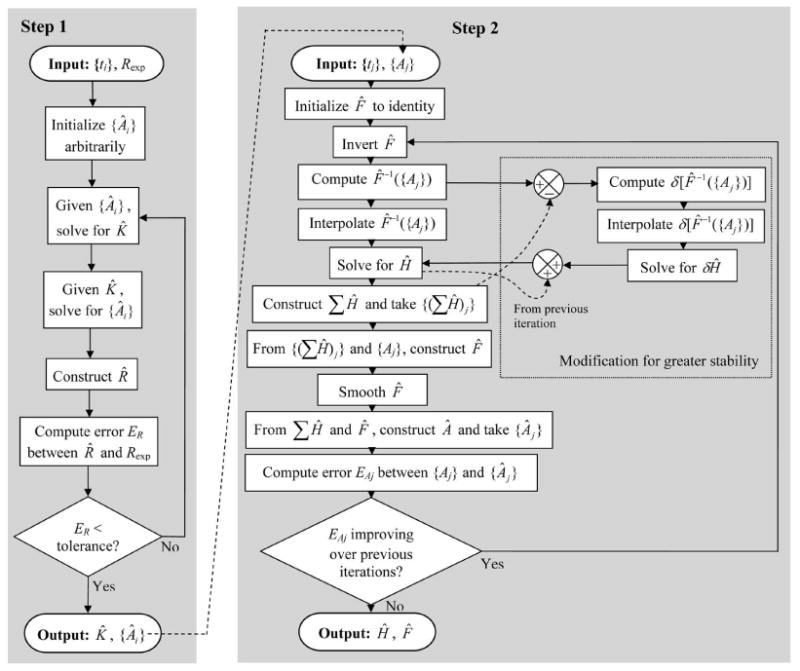
Flowchart of the decoding algorithm. For details see Methods and Supplements 1 and 2.
Step 1: Finding K and A
A complete derivation of the algorithm of Step 1 is provided in Supplement 1. The task of the algorithm is to minimize
with respect to the discrete variables Ai and the continuous function K(t). To simplify the problem, we first discretize time into bins of duration Δt. Thus, t = nΔt, ti = niΔt, Kn = K(nΔt), , where n and ni are integers. Then I0 is replaced by the Riemann sum I:
We also assume that the kernel K is both causal and has finite memory, so that Kn = 0 for n ≤ 0 and also for n > N for some integer N (the “length” of K). Thus, the nonzero values of K are at most K1, …, KN. The task is therefore to minimize I with respect to the N + Ns variables K1, …, KN, A1, …, ANs. This is a calculus problem. To solve it, we differentiate I with respect to each of the variables and set the result equal to 0.
For K, this leads (see Supplement 1) to a linear system of N equations in N unknowns given by
| (3) |
where
for m = 1, …, N and n = 1, …, N. The matrix  (a Toeplitz matrix) is symmetric and positive definite, guaranteeing that the linear system has a unique solution K1, …, KN. However, the solution depends upon the Ai's, which are also unknown.
Similarly, for the Ai's, we have a linear system of Ns equations in Ns unknowns given by
| (4) |
where
for k = 1, …, Ns and i = 1, …, Ns. Since Kn = 0 for n ≤ 0 and for n > N, the sums over n in these definitions of Xki and Yk involve only a finite number of nonzero terms. The matrix X (a banded matrix) is symmetric and positive definite, guaranteeing that the linear system has a unique solution A1, …, ANs. However, this solution depends on K1, …, KN.
Thus, we have a linear system that determines K given A, Eq. 3, and a linear system that determines A given K, Eq. 4. To solve for the values of K and A that simultaneously minimize I, we use the following iterative scheme:
for iteration number l = 0, 1, …. Here (−1Q)(l) is shorthand for the value of −1Q when A = Â(l), and (X−lY)(l) is shorthand for the value of X−1Y when K = K̂(l). To start the iterations, we arbitrarily (see Results) set
for i = l, …, Ns. [We can equally well reverse the order of finding K and A within each iteration and start the iterations with
or 1/N (see Results) for n = 1, …, N.]
For l ≥ 1, the iterative scheme generates an estimate K̂(l) of K and an estimate Â(l) of A. We use these to construct an estimate R̂(l) of R according to
Then we follow the progress of the algorithm by monitoring
| (5) |
Since each step of our iterative scheme finds the optimal value of K or A, given the current estimate of A or K, respectively, it is guaranteed that
Moreover, since I(l) is bounded from below by 0, it is also guaranteed that I(l) converges as l → ∞. In practice, we continue the iterations until I(l) is sufficiently small or until a preset maximal number of iterations is reached.
Performance-enhancing modification
To accelerate the convergence of some decodings (see Results), we smoothed  with a Gaussian kernel density estimation filter (Parzen, 1962; Szücs et al., 2003). In each iteration in which the smoothing was applied, as soon as  was obtained by solving Eq. 4, it was replaced by Â′ given by
| (6) |
The numerator of Eq. 6 is the sum of the values of  and the denominator is the number of the values of  included under the Gaussian smoothing kernel centered on the spike time bin ni of each particular Âi. The standard deviation of the Gaussian kernel, σ, was governed by a function that allowed σ to decrease—the smoothing to weaken—with increasing iteration number l ≥ 1. A typical function was σ = Nt/klp, where Nt is the total number of time bins of Rexp and k and p are constants. For the typical dataset with Ns = 100 spikes at a mean spike rate r = 0.1, and so Nt ≈ 1,000 (see Results), k was set to 20 or 30 and p between 1 (for slowly weakening smoothing) and 2 (for more rapidly weakening smoothing). The smoothing was usually removed entirely after 10-20 iterations. While the smoothing was applied, it was no longer guaranteed that I(l+1) ≤ I(l), although this usually remained true in practice (see Results and Fig. 5).
Fig. 5.

Acceleration of convergence in Step 1 by smoothing of {Âi}. For a train of 100 spikes at r = 0.1, Rexp was constructed from the functions Kexp, Hexp, and Fexp as in Fig. 3A. This same dataset was decoded in all three panels A-C. A: With this dataset, the basic decoding algorithm alone failed to achieve a satisfactory decoding within 80 iterations. Left, the magnitudes of the RMS errors EK (green), EAi (red), and ER (black) in successive iterations, plotted as in Fig. 4. Right, the estimates K̂ and R̂ at 80 iterations (red) superimposed on Kexp and Rexp (blue), plotted as in Fig. 3, B and C, and the estimate {Âi} plotted against {Ai,exp} (top right; the diagonal line is the line of identity). EK was 91.7%, EAi 270.1%, and ER 8.5%. B: With smoothing of {Âi} over the first 15 iterations (gray rectangle) as described in Methods, the same dataset was decoded essentially perfectly. EK was 0.004%, EAi 0.01%, and ER 0.006%. C: A perfect decoding was also achieved when the smoothing was applied later, between iterations 15 and 25. EK was 0.02%, EAi 0.07%, and ER 0.003%. Time is in time bins of duration Δt and amplitude is in arbitrary units.
Step 2: Finding H and F
The presence in Eq. 2 of the nonlinear function F prevents us from applying a strategy like that in Step 1 directly to Eq. 2. However, we can apply it to the simpler equation
In this case, a derivation like that in Step 1 (see Supplement 2) leads to the system
| (7) |
where
for m = 1, …, N and n = 1, …, N. (The matrix  simply counts the spikes with the specified interspike intervals.) This is a linear system of N equations in the N unknowns H1, …, HN.
To use Eq. 7 to find H and at the same time to deal with F, indeed to find F, in the full Eq. 2, we add to the assumptions of our model two further assumptions about F. The first assumption is that F is invertible. In that case, if we know F and so F−1, we can set S(t) = F−1 (A(t)).
Like Step 1, Step 2 therefore proceeds iteratively (see Fig. 2). Before the first iteration, we initialize the estimate of F, F̂, to the identity function, so that S(t) = A(t). We solve Eq. 7 to obtain an estimate of H, Ĥ, and construct [Σj Ĥ](t). We use Eq. 2 to construct F̂ from the pairs ([Σj Ĥ](t), A(t)). Finally, applying F̂ to [Σj Ĥ](t), we construct an estimate of A(t), Â (t).
By themselves, these constructions would produce, of course, Â(t) = A(t). We would have fit A(t) perfectly, but only by collecting all of the error in the underlying F̂ and Ĥ. Furthermore, if we now took F̂−1 to be the inverse of F̂ in this form, the algorithm would cycle through precisely the same values in the next iteration: F̂ and Ĥ would never improve. To improve them, we make a second assumption about F, namely that it is a relatively simple, “smooth” curve with no very sharp changes in slope. When plotted, the raw F̂ is a scatter of points, many of which have very different values of A for similar (even, to a given precision, the same) values of Σj Ĥ, contrary to this assumption. We therefore smooth F̂, and simultaneously F̂−1, using some smoothing filter (see below). The smoothing improves F̂ and so, in the next iteration, also Ĥ. With the smoothed F̂, Â(t) ≠ A(t). The iterations continue as long as the error between Â(t) and A(t) continues to decrease or until a preset maximal number of iterations is reached.
A difficulty in implementing Step 2 exactly as just described is that, to solve Eq. 7 for the time-continuous function H(t), the function S(t) = F−1(A(t)) must likewise be time-continuous. (With discretized time, “continuous” here means “having a value in each time bin.”) However, from Step 1 we know only {Aj}, that is, the values of A(t) sampled only at the spike times {tj}, in general not in every time bin. In each iteration we therefore use only the values at the spike times to construct F̂, and F̂−1 and compute {Sj} = F̂−1 ({Aj}), but then fill in these points by linear interpolation. Even though only {Aj} is known, the algorithm continues to construct the estimate Â(t) of the entire continuous A(t). As a termination criterion, however, we use only the error between the known {Aj} and its estimate {Âj} taken from  (t).
Performance-enhancing modification
In practice we found that the efficacy of the algorithm was significantly greater if we modified each Sj to F̂−1(Aj) − [Σi Ĥ]j, where the last term is the value at the spike time tj of the summed Ĥ constructed in the previous iteration. Now, instead of finding the whole Ĥ anew in each iteration, the algorithm found a residual component, δĤ, that corrected Ĥ from the previous iteration. We routinely implemented this modification as part of the basic algorithm; it is therefore included in Fig. 2.
Investigating the reason for the efficacy of this modification, we found that it was connected with the incomplete knowledge of A(t) just mentioned. If the spikes were so dense that a spike occurred in every time bin, making the complete A(t) available to the algorithm, then Eq. 7 operated analogously to Eq. 3 in Step 1 and the modification was not needed. When the spikes were sparse, however, then Eq. 7 was fitting a waveform, S(t), that consisted predominantly of the values linearly interpolated between the Sj's rather than the Sj's themselves, a waveform that therefore, in general, could never perfectly reflect the true summed H. Thus, even if a perfect solution for H were hypothetically to be found in a particular iteration, that solution would be degraded again in the next iteration. As a result, without the modification, the estimate Ĥ ceased to improve in any systematic way after a small number of iterations. With the modification, however, after the first iteration the residual Sj's were both positive and negative, with many Sj's switching from positive to negative and vice versa in successive iterations; the lines interpolated between the Sj's often passed through zero so that the interpolated values were likewise positive and negative and smaller in absolute terms than the Sj's themselves; and the amplitude of the whole waveform progressively decreased in successive iterations. Each value of the estimate Ĥ was thus built up over the successive iterations as a converging sum of positive and negative terms of progressively decreasing magnitude, allowing essentially any arbitrary shape of Ĥ to emerge fully (provided that the spikes were not so sparse that the interspike intervals exceeded the length of H: see Results).
Smoothing
For smoothing F̂ and F̂−1, we tested several filters and found that the success of the decoding did not critically depend on the filter type. Most of the results presented in this paper were obtained with a Gaussian kernel density estimation filter, analogous to that sometimes used in Step 1, implemented as follows. With F̂ given by the discrete pairs ([Σi Ĥ]j, Aj) as described above, the domain of the corresponding continuous smoothed function F̂′(ΣH) was taken to extend from ΣH = minj ([Σi Ĥ]j) to ΣH = maxj ([Σi Ĥ]j), and F̂′(ΣH) was computed using the equation (analogous to Eq. 6)
| (8) |
In early decodings, we set the standard deviation of the Gaussian kernel, σ, to some fixed fraction of the width of the domain of F̂′, i.e., σ = (maxj([Σi Ĥ]j) − minj([Σi Ĥ]j))/k, where k was typically 30 or 100. In most later decodings, however, we adaptively varied σ so that at each ΣH the value of the denominator of Eq. 8 was always approximately equal to some fixed fraction of the number of spikes, typically Ns/10, Ns/30, or Ns/100. To avoid oversmoothing at the beginning and end of the domain of F̂′ where the discrete values of F̂ were sparse, we sometimes set an upper limit on the value of σ. We found that, within these parameters, the value of σ affected primarily the speed of convergence of the decoding algorithm, without major effect on the final result. After obtaining F̂′ in each iteration, we inverted it and smoothed it by a similar procedure to ensure that F̂′−1, too, was a function.
Two inputs
With two independent inputs 1 and 2 that sum but do not otherwise interact in producing the response (see Results and Fig. 10), the model given by Eqs. 1 and 2 expands to
Fig. 10.

Decoding of two inputs. As in Fig. 3, but with two spike trains, each with its own set of functions Kexp, Hexp, and Fexp, shown in panel A. B: A representative Rexp (blue curve), constructed from the functions in panel A for 200 random spikes with mean rate r = 0.05 from each of the two inputs (empty and filled blue circles along the baseline), then overlaid with the decoded estimate R̂ (red curve). The inset plots R̂ against Rexp. ER was 1.6%. C: The two sets of functions Kexp, Hexp, and Fexp from panel A (blue) overlaid with their decoded estimates K̂, Ĥ, and F̂ (red). EK was 0.13%, EH 14.4%, and EF 3.2% for input 1, and EK 0.25%, EH 7.0%, and EF 1.2% for input 2. Time is in time bins of duration Δt and amplitude is in arbitrary units.
where
and
where ti and tj are the spike times of the two inputs.
To decode this model, in Step 1 we duplicated within each iteration l ≥ 1 all of the steps for finding K and A, first estimating and from {ti}, and , and then estimating and from {tj} and . To initialize the algorithm, we used reconstructed from the estimates K̂ and  that we obtained in an initial decoding of the whole response Rexp with all of the spikes of both inputs combined—that is, from K̂ and  averaged over both inputs—or we simply set . Having found the best estimates of K1, A1, K2, and A2 in Step 1, we then ran Step 2 twice, first to find H1 and F1 from {ti} and A1, and then to find H2 and F2 from {tj} and A2.
Error evaluation
As a measure of the error between the “true” functions and their estimates, we computed throughout this paper the mean-normalized percentage root mean square (RMS) error, symbolized E. In all decodings we computed ER, the error between Rexp and R̂, given by the equation
| (9) |
where Nt is the total number of time bins of Rexp. (Eq. 9 is essentially the normalized percentage RMS form of Eq. 5.) With synthetic data where other true functions were known, errors in the other functions that were defined over time bins—EK, EH, EA (the error in A over all time bins), and EAi or EAj (the errors in A at the spike times only)—were computed analogously to ER. EF was computed similarly between the true F and the smoothed estimate F̂′ over a fixed number (typically 100) of equally spaced values of ΣH covering the domain of F̂′.
The use of RMS error made the errors reported in this paper numerically larger than they would have been if we had computed, for instance, the percentage mean square (MS) error that is often used in Wiener-kernel studies (e.g., Marmarelis and Naka, 1973; Krausz and Friesen, 1977; Sakai, 1992). With the standard normalization (Sakai, 1992), the percentage MS error is approximately equal to E2/100. Thus E = 10% is equivalent to MS error of ∼ 1%, and E = 30% to ∼ 9%. MS error below 10% is usually considered to be very satisfactory (see also numerous examples in Marmarelis, 2004).
Experimental methods
The experiments in Figs. 11 and 12 used the controlled stimulus preparation of the heart of the blue crab, Callinectes sapidus, as described by Fort et al. (2007a). Briefly, the heart was removed from the crab, pinned ventral side up in the dish, and a small window was cut in the ventral wall to expose the trunk of the cardiac ganglion. The ganglion trunk was severed at the midpoint and the anterior portion of the ganglion was removed. The posterior trunk was drawn into a polyethylene suction electrode for extracellular stimulation. Stimulus voltage pulses, delivered from a Grass S88 stimulator, were adjusted (typically between 10-20 V and 1-3 ms) so that each pulse reliably produced a single spike simultaneously in all of the motor neuron axons in the posterolateral connectives. This was confirmed by the detection of a corresponding compound excitatory junctional potential (EJP) in the muscle that did not grow larger when the stimulus parameters were increased. The timing of the stimulus pulses was controlled by a custom-built, computer-based timer capable of generating arbitrarily-timed spike trains. In these experiments random, Poisson spike trains, each consisting of 200-300 spikes at a nominal rate of 2-3 Hz, were repeated with intervening rest periods at least as long as the spike trains themselves. EJPs were recorded with intracellular microelectrodes filled with 2 M KCl (10-30 MΩ) from a part of the muscle that did not move excessively during contractions. Contractions were recorded with a Grass FT03 isometric force transducer connected to the anterior part of the heart with a hook and nylon thread. The preparation was continuously perfused with standard crab saline through its artery.
Fig. 11.

Decoding of real synaptic potentials. A: Top, the decoded dataset, a representative recording of EJP amplitude (intracellularly recorded muscle membrane voltage) in the heart muscle of Callinectes sapidus (blue curve) in response to a train of 273 random motor neuron spikes (blue circles along the baseline) generated by a Poisson process with a nominal rate of 3 Hz. The boxed segment is expanded below. The red curve is the estimate R̂ after both Steps 1 and 2 of the complete decoding. For errors see text. The decoding in Step 1, the reconstruction of R̂, and the computation of ER was performed with a time bin duration Δt = 1 ms, only over the union of the time bins over which K̂ extended after each spike. The decoding in Step 2 was performed with Δt = 10 ms, over all time bins of the dataset. B: The estimates K̂, Ĥ, and F̂ decoded from the dataset in panel A. K̂ is superimposed on a representative scaled single EJP (blue). C: Validation data. The estimates K̂, Ĥ, and F̂ in panel B were used to predict R̂ for a second dataset like that in panel A.
Fig. 12.

Decoding of real muscle contractions. A: Top, the decoded dataset, a representative recording of contraction amplitude (muscle tension) of the heart muscle of Callinectes sapidus (blue curve) in response to a train of 295 random motor neuron spikes (blue circles along the baseline) generated by a Poisson process with a nominal rate of 2 Hz. The boxed segment is expanded below. The green curve shows the estimate R̂ after Step 1 only, the red curve after both Steps 1 and 2. For errors see text. The time bin duration Δt was 10 ms throughout. B: The estimates K̂, Ĥ, and F̂ decoded from the dataset in panel A. K̂ is superimposed on three scaled segments of Rexp (one indicated by the arrow in panel A) where, after an interspike interval just slightly longer than K̂, Rexp had, according to the model, the exact shape of Kexp. C: Validation data. The estimates K̂, Ĥ, and F̂ in panel B were used to predict R̂ for a second dataset like that in panel A.
Results
Synthetic data
To investigate the performance of the decoding algorithm, we first worked with synthetic data, where we knew not only the overall response Rexp but—unlike with real data—also the underlying functions, Kexp, Hexp, and Fexp, from which Rexp had been constructed. We could thus see how good was not just the overall reconstruction R̂ but also the underlying estimates K̂, Ĥ, and F̂—a critical question since it would be those estimates that would then be used to predict the response to any other spike train.
A typical decoding
Fig. 3A shows representative functions Kexp, Hexp, and Fexp, and Fig. 3B shows the response Rexp (blue curve) constructed from them, by the operation of Eqs. 1 and 2 as in Fig. 1, for a train of 100 random spikes (blue dots along the baseline) generated by a Poisson process (Dayan and Abbott, 2001). We used such white-patterned spike trains because the structure of the matrices in Eqs. 3, 4, and 7 suggests that the best decoding will be obtained if all interspike intervals are equally represented. Given only the spike times {ti} and Rexp, the algorithm produced an almost perfect reconstruction R̂, as shown in Fig. 3B by the red curve that exactly overlies the blue curve of Rexp, and the straight-line plot of R̂ against Rexp in the inset. The mean-normalized root mean square (RMS) error between R̂ and Rexp, ER, was 2.0%. At the same time, each of the underlying estimates K̂, Ĥ, and F̂, shown by the red points superimposed on the blue points of Kexp, Hexp, and Fexp in Fig. 3C, was excellent as well. (The RMS errors are given in the legend. As discussed in the Methods, our use of RMS errors, as opposed to mean square (MS) errors, made the error values appear relatively large, and the normalization by the mean increased them further with certain function shapes, such as that of our representative Hexp.)
Fig. 3.

Decoding of synthetic data. A: The three functions Kexp, Hexp, and Fexp that were used to construct the overall response Rexp. B: A representative Rexp (blue curve) constructed, by the operation of Eqs. 1 and 2 as in Fig. 1, for a train of 100 random spikes with mean spike rate r = 0.1 (blue dots along the baseline), then overlaid with its decoded estimate R̂ (red curve). The inset plots R̂ against Rexp. The normalized percentage RMS error between R̂ and Rexp, ER (see Methods), was 2.0%. C: The functions Kexp, Hexp, and Fexp from panel A (blue) overlaid with their decoded estimates K̂, Ĥ, and F̂ (red). The respective RMS errors were EK = 0.008%, EH = 15.0%, and EF = 2.7%. D: Validation data. For a different train of 100 random spikes (blue dots along the baseline), Rexp (blue curve) was again constructed from the functions Kexp, Hexp, and Fexp in panel A, but its estimate R̂ (red curve) was constructed from the functions K̂, Ĥ, and F̂ that were decoded from the first Rexp in panels B, C. ER was 4.8%. Time is in time bins of duration Δt and amplitude is in arbitrary units.
Note, however, that the absolute scaling of the underlying functions does not in fact have a unique solution: without some additional constraint, although the algorithm would have found the correct shapes and the correct relative scaling of the underlying functions, it would not have been able to recover the “true” absolute scaling of each individual function. This is inherent in the structure of the model. In Eq. 1, for instance, K can be multiplied by a constant, k, if {Ai} is multiplied by 1/k. Which k the algorithm settles on depends on the initialization of {Âi}. To permit direct comparison of the shapes of the true and estimated synthetic functions in Fig. 3C and other decodings, we constrained the integrals of Kexp and Hexp, and then of K̂ and Ĥ in each iteration, to be 1. We found, furthermore, that imposing some such constraint on the absolute sizes of K̂ and Ĥ in successive iterations significantly increased the stability and speed of convergence of the algorithm.
Because the estimates K̂, Ĥ, and F̂ were excellent, they were very well able to predict the response to a different spike train with the same nominal statistics (Fig. 3D) or indeed with different statistics.
Performance characteristics of the algorithm
Number of iterations
The matrix implementation of the algorithm solves the entire system of simultaneous equations for all of the values of K̂ (Eq. 3), {Âi} (Eq. 4), and Ĥ (Eq. 7) directly, in one step, and F̂ is also found by a direct construction. No low-level iterative search is necessary. However, each of these estimates is conditional on one (or, in the case of the other models discussed below, more than one) of the other estimates. To improve each estimate in turn, high-level iterations are still required. How many iterations were required to obtain a good decoding? For a decoding like that in Fig. 3, a typical plot of RMS error against iteration number can be seen in Fig. 4. We found that in Step 2 of the algorithm (see Methods) the estimates Ĥ and F̂ converged to practically stable values with low errors after only a few (<10) iterations, whereas in Step 1 the estimates K̂ and {Âi}, although sometimes they converged that rapidly as well, sometimes could take many more iterations (30-100, or even more). In those cases, however, it was often possible to accelerate the convergence, as described next.
Fig. 4.

Magnitudes of the RMS errors E in successive iterations of a decoding like that in Fig. 3, with 100 spikes at r = 0.1 and the same functions Kexp, Hexp, and Fexp as in Fig. 3A. A: The errors EK (green), EAi (red), and ER (black) in Step 1. B: The errors EH (dark blue), EF (light blue), EAj (red), and EA (pink) in Step 2 alone, i.e., when it was given as input the true {Aj,exp} produced by Hexp and Fexp. C: The errors EK (green), EH (dark blue), EF (light blue), and ER (black) in Steps 1 and 2 combined, when Step 2 was given as input the estimate {Âj} from Step 1. EAi, EAj, and EA are the errors between Aexp and  at the spike times {ti} or {tj} or over all time bins, respectively.
Convergence in step 1
In Step 1, the overall error of the reconstruction, ER, always decreased in successive iterations, as it was guaranteed to do until convergence (see Methods). While ER decreased, though, the errors in the estimates of the underlying functions, EK and especially EAi, could increase, as Fig. 4A shows. They often decreased again, as in Fig. 4A, and K̂ and {Âi} did eventually converge. However, the speed of the convergence varied for different spike trains, even with the same nominal statistics, and sometimes K̂ and {Âi} even failed to converge before the maximal number of iterations that we allowed, usually 300, was reached, so that for practical purposes the algorithm failed to solve the problem. Fig. 5A shows such an example (cut off for the purposes of the figure at 80 iterations). Although—as with essentially all decodings, even those that were quite unsatisfactory in other respects—the algorithm achieved a reasonable overall reconstruction R̂, with only 8.5% RMS error (Fig. 5A, right-hand box, bottom plot), the underlying estimates K̂ and {Âi} (right-hand box, top left and top right plots, respectively) were completely incorrect (the RMS errors are plotted in Fig. 5A, left, and given in the legend).
The primary problem lay in the estimation of {Âi}. We calculated the (2-norm) condition numbers for the relevant matrices. Whereas the matrix used to estimate K̂ (see Eq. 3 in Methods) typically had relatively good condition numbers (in decodings like those in Figs. 3-5, of the order of 101 to 102), the matrix X used to estimate {Âi} (see Eq. 4) had poor condition numbers (of the order of 103 to 106). This reflected the fact that whereas the matrix collected the information that yielded each value of K̂ from all parts of the dataset, many of which were so far apart in time that they were essentially independent of each other, the matrix X collected the information that yielded each Âi only from the local environment of that particular spike. (In Step 2, the matrix used to estimate Ĥ in Eq. 7, since it operated like the matrix , likewise had good condition numbers.) As a result—in another ambiguity of decomposition inherent not merely in the model, but in the basic spike-response scenario itself—two spikes close to each other formed a pair whose Âi's traded off against each other. In the limit, two spikes in the same time bin were completely indistinguishable and their Âi's could assume any pair of values, positive or negative, that simply averaged to the same value. A frequent symptom of the problem, therefore, was that even when the true Âi's were all positive, the estimated Âi's were, often rather symmetrically, both positive and negative (Fig. 5A, right-hand box, top left plot). The problem was more severe to the extent that the estimate K̂, too, was poor, and thus most severe in the early iterations of a decoding.
This understanding of the problem suggested at the same time a remedy. For two spikes in the same time bin, the best estimate for both true Ai's is clearly the average of the pair of estimated Âi's. Generalizing this idea, we smoothed the sequence of Âi's, more strongly to the extent that the spikes were close together and most strongly at the beginning of the decoding, weakening over successive iterations before ceasing entirely after 10-20 iterations (for details see Methods). With this smoothing, the same dataset that in Fig. 5A could not be decoded by the basic algorithm alone was decoded perfectly (Fig. 5B). A brief application of the smoothing later in the decoding was equally effective (Fig. 5C). Altogether, we found that in many decodings such smoothing allowed the algorithm to reach practical convergence on sufficiently good values not only of R̂, but of the underlying K̂ and {Âi} as well, after only 10-30 iterations of Step 1, not many more iterations than were required for Step 2.
We emphasize, however, that in Step 1 the smoothing was an auxiliary measure, not an essential part of the algorithm. Indeed, except for Fig. 5, B and C, and several cases in Fig. 7, all of the decodings in this paper were achieved without any Step 1 smoothing. Furthermore, the smoothing appeared merely to accelerate the convergence of the estimates where the convergence was slow due to the ambiguity of nearby spikes just described. It did not alter the final solution that was reached (see next), and where that solution had significant errors due to other causes, these errors remained (we verified this with the decodings of dense spikes in Fig. 6, small numbers of spikes in Fig. 7, and the real data in Figs. 11 and 12).
Fig. 7.

Magnitudes of errors with different numbers of spikes. Synthetic datasets were constructed as in Fig. 3, with r = 0.1 and Rexp constructed from the functions Kexp, Hexp, and Fexp in Fig. 3A, but with different numbers of spikes. Each dataset was decoded for 300 iterations. The errors plotted and their colors are as in Fig. 4. The errors are cut off above 100%. Each point plotted is the median of three runs of the algorithm with three different datasets with that particular number of spikes. With 90 and 190 spikes, essentially arbitrarily in this set of runs, the decoding failed to converge within 300 iterations two out of the three times; for those spike numbers, the algorithm was therefore rerun with the Step 1 smoothing (see Methods and above in Results) and those results are plotted; all other points were obtained without the smoothing. More systematic investigation showed that the Step 1 smoothing also permitted essentially perfect Step 1 decodings to be obtained within 300 iterations already with 20 spikes rather than the 30-40 spikes shown here without the smoothing. However, the basic problem of decoding a dataset with a very small number of spikes remained. A: RMS errors EK (green), EAi (red), and ER (black) in Step 1. B: RMS errors EH (dark blue), EF (light blue), EAj (red), and EA (pink) in Step 2 alone. C: RMS errors EK (green), EH (dark blue), EF (light blue), and ER (black) in Steps 1 and 2 combined.
Fig. 6.

Effects of spike density on the decoding. Synthetic datasets were constructed as in Fig. 3, each with 100 spikes and Rexp constructed from the functions Kexp, Hexp, and Fexp in Fig. 3A, but with different spike densities produced by different spike rates r. A: Typical overall responses Rexp to sparse (r = 0.01), “optimal” (r = 0.1), and dense (r = 1) spike trains. Note the very different absolute time scales and amplitudes in the three cases. Time is in time bins of duration Δt, r is in spikes/Δt, and amplitude is in arbitrary units. B-D: Magnitudes of the RMS errors E in the various decoding estimates, after 300 iterations, as a function of r. Both r and E are plotted on log scales. The horizontal line in each panel, at log E = 0, marks 1% error. Each point plotted is the mean of three runs of the algorithm with three different datasets at that particular r. The errors plotted and their colors are as in Fig. 4. B: The errors EK (green), EAi (red), and ER (black) in Step 1. C: The errors EH (dark blue), EF (light blue), EAj (red), and EA (pink) in Step 2 alone. D: The errors EK (green), EH (dark blue), EF (light blue), and ER (black) in Steps 1 and 2 combined. In panels B and D, the errors are cut off when they decrease below 10−5%.
Uniqueness of solutions
The behavior observed in Fig. 5 might be thought to provide support for the possibility—which we cannot completely rule out theoretically—that the decoding algorithm could admit multiple solutions, multiple minima to which the estimates could converge (in addition to the multiplicity of values of the absolute scaling factor k already mentioned). We believe, however, that in Fig. 5A the estimates were not converging to some alternative (albeit high-error) solution, but rather were very slowly converging to the same low-error solution that was reached rapidly in Fig. 5, B and C. (In practical terms, of course, the result of convergence to an incorrect solution and very slow convergence toward the correct solution is much the same: the dataset is not decoded satisfactorily within a reasonable time.) Thus, although this is imperceptible on the scale used in Fig. 5A, left, the overall error ER continued to decrease slowly even as EK and EAi increased, and when such a decoding was allowed to continue sufficiently long EK and EAi began to decrease too and the decoding eventually reached the low-error solution, behaving as in Fig. 4 but over a much larger number of iterations.
More generally, investigations with a variety of datasets, while necessarily incomplete, suggested that when the estimates in Step 1 did converge, they always converged to the same solution (with the constraint on K̂ already described). For example, the same solution was reached from different random initializations of {Âi} (or K̂). And, at least over some range of dataset parameters, that solution was a global minimum since it had essentially zero error (see further below). Finally, the smoothing was instructive in this regard because it perturbed, not the initial conditions from which the decoding started, but rather the subsequent trajectory of the estimates R̂, K̂, and {Âi}. Following different trajectories, the estimates nevertheless reached the same final solution. This was particularly striking with the real data in Figs. 11 and 12, where the final solution had significant errors, allowing lower-error solutions to be reached if they existed. Nevertheless, not only different initializations of {Âi} or K̂, but multiple trajectories caused by somewhat different smoothing functions all converged to essentially identical final values of R̂, K̂, and {Âi}.
Speed of the algorithm
In MATLAB on a 2.3 GHz Apple MacBook Pro or an equivalent PC, without any special optimization of the code for speed, 300 iterations of a decoding like that in Fig. 3 took several minutes. Thus a sufficiently good decoding, requiring only a small number of iterations, could often be achieved in seconds.
Forms of K, H, and F
For convenience, the functions in Fig. 3A were generated using analytic functions—an α-function (Dayan and Abbott, 2001) for Kexp, an exponential for Hexp—but the functions were actually defined as the vectors of their numerical values, the dots in Fig. 3A. Quite arbitrary functions could therefore be used to construct Rexp (see, e.g., Fig. 10 below). Since the algorithm treats each function value as an independent degree of freedom, and the initialization of the function estimates is arbitrary, the algorithm was able to decode such functions just as successfully as those in Fig. 3. We verified this with a wide range of functions. If Kexp had multiple peaks, for example, the algorithm successfully decoded the corresponding complex K̂, distinguishing those peaks of Rexp that were inherent to Kexp from those that arose by the summation of the Kexp's of different spikes (see Fig. 10).
Spike density
While the algorithm successfully decoded datasets like those in Fig. 3, its success varied with several parameters of the dataset. Chief of these was the spike density. For the decoding problem, spike density is significant not in absolute terms, but relative to the characteristic time scales of the response, here those of Kexp and Hexp. By varying the mean rate r (expressed in spikes per time bin) of the spike train relative to the fixed time scales of Kexp and Hexp, we generated sparse spike trains with overall responses Rexp in which the individual kernels Kexp hardly overlapped at all (Fig. 6A, left), or, on the other hand, dense spike trains where the individual Kexp's fused almost completely into a summated, plateau-like Rexp (Fig. 6A, right).
Fig. 6B-D then plots the RMS errors E in various estimates produced by the algorithm, after 300 iterations, against log r. The errors too are plotted on a log scale; the horizontal line in each panel, at log E = 0, marks 1% error, a very satisfactory decoding. Panel B shows the errors in K, {At}, and R in Step 1. Panel C shows the errors in H, F, {Aj}, and the entire A(t) in Step 2 when Step 2 was run alone, that is, when it was given as input the true {Aj,exp} produced by Hexp and Fexp. Finally, panel D shows the errors in K, H, F, and R when both Steps 1 and 2 were run in combination—as they were in a complete decoding like that in Fig. 3—in which case Step 2 had available to it only the estimate {Âj} from Step 1 and so inherited any error of Step 1. We can see in these plots three regions of qualitatively different performance of the algorithm.
(1) With very dense spikes, to the right toward r = 1, the algorithm reconstructed the overall input, Rexp in Step 1 and {Aj} in Step 2, very well, often with errors ≪1%. But it did this with poor estimates of the underlying functions, which would therefore have been unsuccessful in predicting the responses to other (sparser) spike trains.
(2) With very sparse spikes, to the left toward r = 0.01, the decoding in Step 1 was (with this noise-free data) essentially perfect. The algorithm dealt perfectly with a single spike, when Kexp and Ai were evident simply by inspection, and with several spikes with nonoverlapping responses, when it simply averaged the responses. The decoding in Step 2, however, was much poorer, for a fundamental reason. Information about the underlying functions Hexp and Fexp is sampled, in the form of {Aj}, only at the spike times. If the spikes are so sparse that each spike comes only after Hexp of the previous spike has completely decayed, then {Aj} contains no information at all about Hexp and Fexp, and they cannot be recovered.
(3) Between the sparse and dense regions there was an “optimal” region, around r = 0.1 with the time scales of Kexp and Hexp used here, where the range of interspike intervals was such that the overall response Rexp contained a variety of shapes and sampled a broad range of amplitudes (Fig. 6A, middle). (The datasets in Fig. 3 had r = 0.1.) In this region, the errors in all estimates were satisfactory: ≪1% in Step 1, close to 1% in Step 2 alone, and often not much higher in the complete decoding. In this region, on average, every 10th time bin contained a spike. Thus, only 10% of A(t) was sampled by {Aj}. Nevertheless, the algorithm reconstructed the entire continuous A(t) within 1% error, as it had to do to be able to predict the response to a spike that would be fired, in a future spike train, at any arbitrary time.
Number of spikes
The decodings in Figs. 3-6 were performed with 100 spikes. How many spikes were actually required for a good decoding? We performed similar decodings while varying the number of spikes, generated at the “optimal” r = 0.1, from 10 to 1000. The RMS errors up to 200 spikes can be seen in Fig. 7. With very few spikes, the decoding was poor, particularly in Step 2. However, errors not much higher than those in Fig. 3 were achieved already with 40 or 50 spikes. The errors then continued to decrease slowly as the number of spikes was increased further.
At the same time, of course, the increasing number of spikes, and the corresponding increase in the number of time bins of Rexp, increased the computational burden. At the core of the algorithm, Eqs. 3, 4, and 7 involve the construction and manipulation of numerical arrays whose size increases with the number of spikes Ns and the number of time bins Nt ≈ Ns/r of Rexp (as well as the lengths of K̂ and Ĥ). With 1000 spikes, a decoding allowed to run for the full 300 iterations could take several hours.
Noise
All of the results so far were obtained with noise-free datasets. The quality of the decoding might be expected to degrade with noise. We examined this in three ways. We added random noise to the value of the overall response Rexp in each time bin; we added random noise to each value of the underlying functions Kexp, Hexp, and Fexp; and we added random noise to parameters of the analytic functions that (for this purpose only) were used to generate the underlying functions at each spike time, for example to the time constant of Kexp, so that the whole shape of Kexp fluctuated from spike to spike. The results were similar in all three cases. For the addition of noise to Rexp, for example, a typical decoding can be seen in Fig. 8, and a plot of the RMS errors in the decoded estimates against the RMS amplitude of the noise can be seen in Fig. 9. The quality of K̂ and R̂ degraded quite gently with increasing noise; that of Ĥ and F̂, presumably because of the smoothing of F̂, did not degrade at all. Even with substantial noise, the algorithm was able to estimate roughly correct forms of K̂, Ĥ, and F̂ and to reconstruct an overall R̂ that approximated not so much the noisy Rexp that the algorithm was given to decode, but the underlying noise-free Rexp (see Fig. 8). Thus, the algorithm is robust against these kinds of noise. This reflects its strongly averaging nature. Inspection of Eqs. 3, 4, and 7, for example, reveals how they combine information from many spikes and values of Rexp to construct each estimated value and thus filter out random perturbations.
Fig. 8.

Decoding of noisy synthetic data. As in Fig. 3, but with random noise added to the overall response Rexp before decoding. A noise-free Rexp, for 200 spikes at r = 0.1 in these datasets, was first constructed from the functions Kexp, Hexp, and Fexp in panel A, identical to those in Fig. 3A. In each time bin, a different random number drawn from a Gaussian distribution with zero mean and a given standard deviation was then added to the noise-free Rexp to construct a noisy Rexp (blue curve in panel B). The RMS amplitude of the noise, that is, the RMS difference between the noise-free and noisy Rexp, was computed analogously to the RMS error ER using the equivalent of Eq. 9. In panel B, the amplitude of the noise was 22.1%. The algorithm then decoded the noisy Rexp to estimate R̂ (red curve in panel B). The inset in panel B plots R̂ against the noisy Rexp (black dots) as well as against the underlying noise-free Rexp (red dots). The error ER of R̂ relative to the noisy Rexp was 25.2%, but relative to the noise-free Rexp only 12.4%. In panel C, EK was 31.6%, EH 9.8%, and EF 1.7%. For the validation data in panel D, the noise amplitude was 24.1%, ER relative to the noisy Rexp 24.9%, and ER relative to the noise-free Rexp 11.9%. Time is in time bins of duration Δt and amplitude is in arbitrary units.
Fig. 9.

Magnitudes of errors with different amplitudes of noise. Synthetic datasets were constructed as in Fig. 8, with 200 spikes at r = 0.1 and the noise-free Rexp constructed from the functions Kexp, Hexp, and Fexp in Fig. 8A, but with different RMS amplitudes of noise added to construct the noisy Rexp. Each dataset was decoded for 300 iterations. Plotted are the RMS errors EK (green), EH (dark blue), EF (light blue), and ER relative to the noise-free Rexp (black) in Steps 1 and 2 combined. For each nominal noise amplitude, the algorithm was run three times; the point plotted is that with the lowest ER.
Other models
By combining building-block functions like K, H, and F in different ways, many other models can be built. We tested the decoding algorithm, with appropriate modifications, on several classes of such models, including the following models in which Eq. 1 was replaced by one of the Eqs. 10-12, then combined with one or two instances of Eq. 2:
| (10) |
| (11) |
where G is another nonlinear, invertible, and “smooth” function, and
| (12) |
where ti and tj are the spike times of two different inputs with different functions K and A.
With essentially all models tested, the algorithm found some set of estimates of the underlying functions that reconstructed the overall Rexp well. With some of the model classes, however, the underlying estimates were clearly not unique and therefore, in general, not correct. Models containing Eqs. 10 and 11 were in this category. As with the trade-off between K and A in Eq. 1, the lack of uniqueness was inherent already in the structure of the equations.
In contrast, with the additional information provided by the two distinct spike trains in Eq. 12, models of this class were completely decodable. This can be seen in Fig. 10. Here the overall Rexp (blue curve in panel B) was constructed as the summed response to two simultaneous random spike trains from two independent inputs (empty and filled blue circles along the baseline), each acting through its own set of functions Kexp, Hexp, and Fexp (panel A). Nevertheless, given just Rexp and the two sets of spike times {ti} and {tj}, the algorithm reconstructed Rexp essentially perfectly (red curve in panel B) and in the process correctly extracted all six of the underlying functions (panel C).
Likewise completely decodable, in principle, were cascade models of the form
Real data
We now describe the decoding of two kinds of real neurophysiological data. Both sets of data were recorded in a standard invertebrate preparation, the crustacean heart (Cooke, 2002), here that of the blue crab, Callinectes sapidus (Fort et al., 2004, 2007a,b). In the neurogenic crustacean heart, trains of motor neuron spikes drive synaptic depolarizations and contractions of the heart muscle. Endogenously, the spikes occur in bursts. In both datasets, however, we stimulated the motor neurons to produce instead white-patterned spike trains as in the synthetic data. As the response, in one dataset we recorded the synaptic potentials—more correctly, the excitatory junctional potentials (EJPs)—that the spikes elicited in the heart muscle, and in the other dataset the subsequent muscle contractions. In both cases, we used the model given by Eqs. 1 and 2 for the decoding.
Synaptic potentials
Fig. 11A, top, shows the entire decoded dataset, consisting of 273 random motor neuron spikes (blue circles along the baseline) and the resulting Rexp of muscle EJPs (blue curve). A representative segment is expanded below, overlaid with the estimate R̂ after both Steps 1 and 2 of the complete decoding (red curve). Over the entire dataset, the RMS error ER was 35.6%. Most of this error originated in Step 1, where ER was 27.2%, whereas the error in the decoding of {Aj} in Step 2 was only 15.5%. At first glance, these errors seemed high. In part, however, they appeared high because they were RMS, as opposed to MS, errors. Allowing for this, a decoding with these errors was in fact quite satisfactory when compared to those obtained by other methods (cf., e.g., Marmarelis and Naka, 1973; Krausz and Friesen, 1977; Sakai, 1992; Marmarelis, 2004; Song et al., 2009b). Nevertheless, we computed some benchmark values. By recording the response to the same spike train several times, we found that the intrinsic RMS variability of the recording and preparation, which ER cannot be expected to improve upon, was 33.0%. At the other end of the scale, if we had no model at all and “predicted” Rexp simply by its own mean, ER, equivalent in this case to the coefficient of variation of Rexp, was 127.2%. Thus, the ER of the decoding was in fact close to the low end of the possible range.
The decoded estimates K̂, Ĥ, and F̂ are shown in Fig. 11B. K̂ is overlaid on, to show that it closely resembles, one representative EJP cut from Rexp. Ĥ has a complex, biphasic shape. If H is interpreted as reflecting processes of presynaptic plasticity at the neuromuscular junction (Magleby and Zengel, 1975, 1982; Krausz and Friesen, 1977; Zengel and Magleby, 1982; Sen et al., 1996; Hunter and Milton, 2001; Zucker and Regehr, 2002) that determine the amount of transmitter released, A, then the early negative phase of Ĥ can be interpreted as a brief depression of potential transmitter release after each spike, perhaps due to temporary depletion of the immediately releasable pool of transmitter (Hunter and Milton, 2001; Zucker and Regehr, 2002). The later positive phase of Ĥ then reflects facilitation of the transmitter release. With the fast, largely nonsummating EJPs, the depression could indeed be observed in pairs of EJPs simply in the raw recording (e.g., in Fig. 11A), and both depression and facilitation have been observed at this neuromuscular junction with regular spike patterns incorporating different interspike intervals such as are conventionally used to study synaptic plasticity (Fort et al., 2005, 2007a).
The estimates K̂, Ĥ, and F̂ were equally well able to predict the response to a new train of spikes. Over the entire new dataset in Fig. 11C, top, ER was 39.0%, not much higher than over the original dataset.
Muscle contractions
Because of the overlap and summation of the much slower muscle contractions, we expected that they would present a much more challenging decoding problem. Fig. 12A, top, shows the entire decoded dataset, consisting of 295 random motor neuron spikes (blue circles along the baseline) and the resulting Rexp of heart muscle contraction amplitude (blue curve). A representative segment is expanded below, overlaid with the estimate R̂ after Step 1 only (green curve) and after both Steps 1 and 2 of the complete decoding (red curve). Over the entire dataset, the RMS error ER was only 7.1% after Step 1 and 28.9% after both Steps 1 and 2. As with the sparse synthetic datasets (Fig. 6), the error was significantly higher in Step 2 than in Step 1, and so also in the complete decoding, presumably because of the incomplete sampling of A(t) in Eq. 2 by the sparse spikes, but also, perhaps, because Eq. 2 may not be the optimal model for this part of the real transform. The intrinsic variability of the preparation was 8.0% and the coefficient of variation of Rexp was 69.3%.
The decoded estimates K̂, Ĥ, and F̂ are shown in Fig. 12B. K̂ is overlaid on, and closely resembles, three segments of Rexp in which the shape of Kexp could be identified (see legend). Ĥ, remarkably, has the same complex, biphasic shape as that decoded from the EJP data in Fig. 11B. Thus, the history kernel H of the overall neuromuscular transform has a synaptic, and probably presynaptic, origin. However, where the F̂ in Fig. 11B never produces EJPs of zero amplitude, the F̂ in Fig. 12B does produce zero-amplitude contractions, suggesting most likely a threshold nonlinearity in the final step of the transform from EJPs to contractions. The complex shape of Ĥ has interesting implications for the case of the endogenous spike pattern, where the spikes are generated in bursts with ∼ 7 spikes per burst, ∼ 40 ms between the spikes in the burst, and ∼ 2.5 s between bursts (Fort et al., 2004). Each spike inhibits the response to the subsequent spikes in the same burst, and the entire burst would produce little contraction response were it not preceded, by an interval well matched to the positive phase of Ĥ, by the previous burst. Thus at the natural frequency of the cardiac rhythm each burst not only produces a contraction, but sets up the conditions that allow a contraction to be produced by the next burst.
The estimates K̂, Ĥ, and F̂ were equally well able to predict the contraction response to a new train of spikes. Over the entire new dataset in Fig. 12C, top, ER was 30.0%, and over the last 100 spikes of the dataset (reflecting a noticeable nonstationarity in each of these datasets) it was just 21.2%.
Discussion
The decoding method: its advantages and limitations
We have described here a method for nonlinear system identification of the transform from a discrete spike train to a continuous neurophysiological response. Based on the “synaptic decoding” approach of Sen et al. (1996) and Hunter and Milton (2001), our method combines elements of traditional model-based methods and model-free methods such as the Volterra or Wiener kernel approach. Like the latter methods, our method begins by finding the first-order, linear kernel of the system (K). Instead of computing higher-order kernels, however, our method then combines the first-order kernel with a small number of additional linear kernels and nonlinear functions (in our illustrative model, H and F) to characterize the system's nonlinearities. Like traditional model-based methods, our method thus fits to the data a model with a certain structure. Mathematical analysis of the model is used to find an efficient fitting algorithm that can be optimally implemented with linear-algebra techniques. Like most other methods, the method assumes stationarity of the system over the duration of the decoded dataset (the method finds averages over that duration), finite memory (finite length of K and H), and causality (K and H only operate after each spike).
The method's combination of model-based and model-free elements, and the analytical and linear-algebra techniques of solution, have a number of advantages but also some limitations.
Like the model-free Volterra or Wiener kernel approach, the method can take advantage of the benefits of white-patterned spike input (see Sakai, 1992; Marmarelis, 2004), yet such input is not strictly required. For example, we have been able to decode the crab heart neuromuscular transform even with the endogenous bursting spike patterns (Stern et al., 2007a).
The basic structure of the model must be chosen in advance. Since any chosen structure, unless it is completely general, will fit only a subset of systems, the need for a model means that the method cannot a priori guarantee a completely general description of any arbitrary system. The manner in which our illustrative model, in particular, departs from the completely general model that is implicit in the Volterra or Wiener kernel approach is discussed further below. It is furthermore possible (as we saw in the Results) to choose a model that is more complex than is justified by the information available in the single overall response Rexp. The model is then underconstrained by the data: multiple solutions are possible and, without additional information, cannot be distinguished. This difficulty is, however, common to all methods that involve a model.
It is in its relative freedom from a priori assumptions and efficient techniques of solution where the method compares most advantageously with traditional model-based methods as well as the previous decoding methods of Sen et al. and Hunter and Milton. In contrast to traditional model-based methods, once the basic model is chosen, apart from the assumption that its static nonlinearities such as F are invertible and smooth, no specific assumptions need to be made about the forms of its kernels and functions. The forms emerge automatically from the computation. Each numerical function value is treated as an independent degree of freedom and is initially set arbitrarily. All of the values of each function are found in one step by solving a matrix equation or by direct construction, and for that step the solution can, in many cases, be proved to be globally optimal. High-level iterations are still required because the solution for each function is conditional on estimates of the others. However, extensive low-level iterations to find the individual function values are not required. For many practical applications, this is likely to be a decisive advantage. One limitation, however, is that some models may not be readily amenable to the mathematical analysis required to separate the functions into the individual linear matrix equations. For example, models in which the single-spike response kernel K does not have a fixed shape, but changes shape in some manner that is more complex than the simple scaling in Eq. 1, may be difficult to solve.
To make this discussion more concrete, it is worth comparing our method to the previous methods of Sen et al. and Hunter and Milton in more detail. Since both Sen et al. and Hunter and Milton used models similar to our illustrative model, we will discuss their methods in terms of our functions K, H, F, A, and R. Both Sen et al. and Hunter and Milton obtained the kernel K simply by taking the shape of an isolated response to a single spike. Deconvolving K from Rexp then gave the Ai's, solving our Step 1 essentially by inspection. Hunter and Milton note that extracting the Ai's rather than working with the entire continuous R “reduce[d] the computation time by two to three orders of magnitude for a 30 sec spike train.” We did not wish to take this shortcut because of its lack of generality: although it would have been possible to do it with the EJPs in Fig. 11, it would have been difficult with the contractions in Fig. 12 and impossible with any denser response waveform. From the Ai's, Sen et al. and Hunter and Milton then found H and F by a gradient descent optimization coupled with the earliest possible assumption, guided where possible also by prior knowledge of the specific synaptic system under investigation, of likely simple forms for these functions, for example exponential for H and low-order polynomial for F, whose few parameters were then found in the optimization. Taking the less automated procedure of Sen et al. as an example, this involved a nesting of the low-level iterations of the gradient descent optimization itself within a series of high-level iterations. First, Sen et al. divided H in a piecewise manner—essentially as we did here—and used gradient descent to find an initial approximation of each piece. Then, substituting a simple function that appeared best to describe the emerging H, they used gradient descent again to optimize the parameters of that function, then of F, which was constructed much like our F and then described by a simple function, and finally of both H and F together. With our method, in contrast, we find the best current estimates of the full shapes of K, H, and F in one step in each high-level iteration, without any simplification of these shapes or dependence on any initial guess. On the other hand, essentially any model that can be postulated, even if it is in fact more complex than is justified by the data and has multiple solutions, can be solved by gradient descent optimization, in the sense that some solution, which with simple function forms will furthermore appear to be plausible, will emerge. Under the same circumstances, our method may not be able to solve the matrix equations for numerical reasons, or, if a solution does emerge, the many degrees of freedom allowed by the many individual values of the functions K, H, and F will produce what is clearly an implausible solution (as in Fig. 5A, for example). This may be valuable, however, as an explicit warning of a problem in the relationship of the model to the data.
In the full Volterra or Wiener kernel approach, the higher-order kernels are abstract descriptions of the structure of the dataset (Sakai, 1992; Marmarelis, 2004) that can typically be interpreted mechanistically only if a traditional, specific model of the system is also postulated (e.g., Song et al., 2009a,b). In contrast, a model with a basic internal structure such as is decoded by our method can itself be immediately interpreted in terms of the underlying physiological mechanisms. Interpreting our illustrative model in neuromuscular terms, as we have done here, H can plausibly be identified with the presynaptic processes of facilitation and depression of transmitter release, A with the amount of transmitter actually released at each spike, and K with the postsynaptic electrical response (when the EJPs are taken as the response) and the Ca2+ elevation and contractile processes in the muscle (when the muscle contractions are taken as the response). F reflects the static nonlinearities of the entire pathway. Such interpretations can then be pursued experimentally. Better models can be identified by their better fit to data that emphasize different aspects of the physiological mechanism. The forms of the model functions can be compared across different synapses or muscles (Sen et al., 1996) or after modification by neuromodulators (Stern et al., 2007a). In the crab cardiac system, we have already extended our analysis in some of these ways and developed the basic decodings presented in this paper into a more definitive characterization of the crab cardiac neuromuscular transform (Stern et al., 2007a,b, 2008; manuscript in preparation).
Relationship to LNL and other cascade structures
Although our method can solve various models, in this paper we have worked mainly with the illustrative model given by Eqs. 1 and 2. This model is of a similar degree of generality to, and indeed in structure closely resembles, the various block-structured cascades of dynamic linear and static nonlinear elements that have been studied extensively as general models of nonlinear biological systems and previously solved by various methods, notably methods based on information about these structures that is contained in the kernels of the Volterra or Wiener expansion (Korenberg et al., 1988; Korenberg, 1991; Sakai, 1992; Westwick and Kearney, 2003; Marmarelis, 2004).
Superficially, our illustrative model appears identical to the LNL (also called “sandwich” or Korenberg) cascade, a serial structure of a dynamic linear element, a static nonlinearity, and then another dynamic linear element (Korenberg and Hunter, 1986; Westwick and Kearney, 2003; Marmarelis, 2004). In our model, these elements are H, F, and K, respectively. However, our model is not a purely serial cascade. The input spike train enters the model in two places, not only at the beginning of the cascade, at Eq. 2 where each spike elicits an instance of H, but also later at Eq. 1 where each spike elicits an instance of K. This creates an additional, parallel branch in the structure (as can be seen, for example, in the schema on the left-hand side of Fig. 1B). Furthermore, where the two branches join at Eq. 1, they do not join additively as is typically modeled in parallel cascades (Korenberg, 1991; Westwick and Kearney, 2003), but rather multiplicatively. This can be seen if, for better comparison with the time-continuous cascade models, we likewise generalize our model to the continuous case. In that case, the spike train becomes a continuous waveform, T, given by a sum of delta functions at the spike times (or, in discretized time, a sequence of integers denoting the number of spikes in each time bin). Over all time points t, t′, Eq. 1 then generalizes to the equation
| (13) |
that is, a convolution of K with the product AT. (Eq. 2 generalizes similarly.) The spikes thus multiplicatively gate the flow of A to produce R, and conversely, when decoding R, their absence hides the processes that produced A from view, giving rise to some of the decoding problems that we encountered in the Results. All of these features make our model significantly different from the pure LNL cascade (it becomes a pure LNL cascade only in trivial cases, such as when T(t) = 1) and make difficult its solution by the previous methods used with such cascades.
Although our decoding method was developed for the case of discrete, relatively sparse spikes, and realizes considerable computational benefits by focusing only on the times when spikes occur, it can also solve the continuous case, such as given by Eq. 13, the continuous generalization of Eq. 2, or Eq. 14 below. Therefore, our method can solve the general LNL cascade. Interestingly, in achieving the solution in two separable steps, first Step 1 to find K and the intermediate function A, and then Step 2 to find H and F, our method would appear to be significantly simpler than the method of Korenberg and Hunter (1986), for example, that iteratively improves the estimates of all three functions in turn.
Our Eq. 2 (especially in the continuous case) is fully equivalent to a subset of the LNL cascade, the LN (also called Wiener) cascade that consists just of a dynamic linear element followed by a static nonlinearity (Sakai, 1992; Westwick and Kearney, 2003; Marmarelis, 2004). Our method of solving Eq. 2 in Step 2 is essentially equivalent to that used by Hunter and Korenberg (1986) to solve LN cascades, except that we have substituted smoothing for their fitting of a high-order polynomial.
As this discussion implies, neither a single LNL cascade nor our illustrative model is completely general in the sense of being sufficient to represent the dynamics of any nonlinear dynamical system. That requires a structure of multiple parallel LNL cascades, LN cascades, or L elements all feeding into a multi-input nonlinearity (the last structure being called the Wiener-Bose model). A sufficient number of these elements can represent any system to any arbitrary degree of accuracy, and has an associated Volterra or Wiener kernel representation, which thus can provide a completely general description of the system (Palm, 1979; Korenberg, 1991; Westwick and Kearney, 2003; Marmarelis, 2004; Song et al. 2009a).
Further applications
Although in this paper we have used data from a neuromuscular synapse, there is nothing inherently synaptic or neuromuscular about our decoding method. We anticipate that it may be useful wherever trains of spikes elicit continuous responses of any kind that can be regarded as being built up of discrete, relatively invariant single spike responses. This includes, for example, responses of intracellular signals such as cAMP and Ca2+, which can be recorded with the requisite temporal resolution (see, e.g., Kreitzer et al., 2000; Augustine et al., 2003; Nikolaev and Lohse, 2006). The method can also be used to decode, from a spike train and a continuous firing rate function constructed from the very same spike train, functions like H and F that characterize how past spikes influence the generation of future spikes in an autonomously active, for example a regularly bursting, neuron (Brezina et al., 2008).
Furthermore, as was pointed out for their method by Sen et al. (1996), the method may also be applicable to the inverse sensory problem, which seeks to understand how continuous sensory stimuli are encoded in discrete spike trains and how, from those spike trains, the central nervous system then decodes or reconstructs the sensory stimuli again (Rieke et al., 1997; Simoncelli et al., 2004). Linear filters such as K are the basis of reverse-correlation (Ringach and Shapley, 2004) and stimulus-reconstruction (Rieke et al., 1997) techniques, and more elaborate models of sensory encoding (Simoncelli et al., 2004; Pillow et al., 2005) add nonlinearity using building blocks like those of Eqs. 1 and 2. As we have already noted, our method generalizes to cases where both stimulus and response are continuous, such as the equation
| (14) |
where S(t) is, say, a sensory stimulus and R(t) the response to it, such as the spike rate of a responding neuron. Knowing S and K, we can predict R (sensory encoding); knowing S and R, we can, in one step using a generalized Eq. 3, find K (the problem usually addressed by reverse correlation); and knowing K and R, we can, in one step using a generalized Eq. 4, reconstruct the stimulus S.
The inverse problem arises, indeed, even with the spike-response transforms that we have considered here in the forward direction. Here, having characterized a transform, we predicted the response to a given spike train. However, we may well wish to reconstruct, conversely, the spike train that has produced a given response. And, by virtue of the global matrix formulation of the equations of the transform, this inverse computation, too, can be readily accomplished. In preliminary work, we have used the discrete Eq. 4 or its continuous version, as applicable, to reconstruct spike trains from synthetic response waveforms as well as the EJP and contraction response waveforms recorded in the real crab heart (Brezina et al., 2009; manuscript in preparation).
Supplementary Material
Acknowledgments
Supported by NIH grants NS058017, NS41497, GM08224, and RR03051. We thank Aaron Lifland for help with implementation of the arbitrary spike timer used in Figs. 11 and 12.
Footnotes
Publisher's Disclaimer: This is a PDF file of an unedited manuscript that has been accepted for publication. As a service to our customers we are providing this early version of the manuscript. The manuscript will undergo copyediting, typesetting, and review of the resulting proof before it is published in its final citable form. Please note that during the production process errors may be discovered which could affect the content, and all legal disclaimers that apply to the journal pertain.
References
- Augustine GJ, Santamaria F, Tanaka K. Local calcium signaling in neurons. Neuron. 2003;40:331–346. doi: 10.1016/s0896-6273(03)00639-1. [DOI] [PubMed] [Google Scholar]
- Brezina V, Orekhova IV, Weiss KR. The neuromuscular transform: the dynamic, nonlinear link between motor neuron firing patterns and muscle contraction in rhythmic behaviors. J Neurophysiol. 2000;83:207–231. doi: 10.1152/jn.2000.83.1.207. [DOI] [PubMed] [Google Scholar]
- Brezina V, Stern E, García-Crescioni K, Miller MW, Peskin CS. Computing the inverse of the neurophysiological spike-response transform. BMC Neuroscience. 2009;10(Suppl 1):P92. doi: 10.1016/j.jneumeth.2009.07.034. [DOI] [PMC free article] [PubMed] [Google Scholar]
- Brezina V, Stern E, Lifland AW, García-Crescioni K, Fort TJ, Miller MW, Peskin CS. 2008 Abstract Viewer. Washington, DC: Society for Neuroscience; 2008. Decoding of simple kernel-based spike train models. Program 695.14. online. [Google Scholar]
- Cooke IM. Reliable, responsive pacemaking and pattern generation with minimal cell numbers: the crustacean cardiac ganglion. Biol Bull. 2002;202:108–136. doi: 10.2307/1543649. [DOI] [PubMed] [Google Scholar]
- Dayan P, Abbott LF. Theoretical Neuroscience. Cambridge, MA: MIT Press; 2001. [Google Scholar]
- Fort TJ, Brezina V, Miller MW. Modulation of an integrated central pattern generator-effector system: dopaminergic regulation of cardiac activity in the blue crab Callinectes sapidus. J Neurophysiol. 2004;92:3455–3470. doi: 10.1152/jn.00550.2004. [DOI] [PubMed] [Google Scholar]
- Fort TJ, Brezina V, Miller MW. Regulation of the crab heartbeat by FMRFamide-like peptides: multiple interacting effects on center and periphery. J Neurophysiol. 2007a;98:2887–2902. doi: 10.1152/jn.00558.2007. [DOI] [PubMed] [Google Scholar]
- Fort TJ, García-Crescioni K, Agricola HJ, Brezina V, Miller MW. Regulation of the crab heartbeat by crustacean cardioactive peptide (CCAP): central and peripheral actions. J Neurophysiol. 2007b;97:3407–3420. doi: 10.1152/jn.00939.2006. [DOI] [PubMed] [Google Scholar]
- Fort TJ, Krenz W, Brezina V, Miller MW. 2005 Abstract Viewer. Washington, DC: Society for Neuroscience; 2005. Modulation of the crab cardiac system: assessment of synaptic transmission with controlled stimulus trains. Program 752.23. online. [Google Scholar]
- Gamble ER, DiCaprio RA. Nonspiking and spiking proprioceptors in the crab: white noise analysis of spiking CB-chordotonal organ afferents. J Neurophysiol. 2003;89:1815–1825. doi: 10.1152/jn.00977.2002. [DOI] [PubMed] [Google Scholar]
- Hunter IW, Korenberg MJ. The identification of nonlinear biological systems: Wiener and Hammerstein cascade models. Biol Cybern. 1986;55:135–144. doi: 10.1007/BF00341929. [DOI] [PubMed] [Google Scholar]
- Hunter JD, Milton JG. Synaptic heterogeneity and stimulus-induced modulation of depression in central synapses. J Neurosci. 2001;21:5781–5793. doi: 10.1523/JNEUROSCI.21-15-05781.2001. [DOI] [PMC free article] [PubMed] [Google Scholar]
- Johnston D, Wu SMS. Foundations of Cellular Neurophysiology. Cambridge, MA: MIT Press; 1995. [Google Scholar]
- Katz B. The Release of Neural Transmitter Substances. Liverpool: Liverpool University Press; 1969. [Google Scholar]
- Korenberg MJ. Parallel cascade identification and kernel estimation for nonlinear systems. Ann Biomed Eng. 1991;19:429–455. doi: 10.1007/BF02584319. [DOI] [PubMed] [Google Scholar]
- Korenberg MJ, French AS, Voo SKL. White-noise analysis of nonlinear behavior in an insect sensory neuron: kernel and cascade approaches. Biol Cybern. 1988;58:313–320. doi: 10.1007/BF00363940. [DOI] [PubMed] [Google Scholar]
- Korenberg MJ, Hunter IW. The identification of nonlinear biological systems: LNL cascade models. Biol Cybern. 1986;55:125–134. doi: 10.1007/BF00341928. [DOI] [PubMed] [Google Scholar]
- Krausz HI, Friesen WO. The analysis of nonlinear synaptic transmission. J Gen Physiol. 1977;70:243–265. doi: 10.1085/jgp.70.2.243. [DOI] [PMC free article] [PubMed] [Google Scholar]
- Kreitzer AC, Gee KR, Archer EA, Regehr WG. Monitoring presynaptic calcium dynamics in projection fibers by in vivo loading of a novel calcium indicator. Neuron. 2000;27:25–32. doi: 10.1016/s0896-6273(00)00006-4. [DOI] [PubMed] [Google Scholar]
- Magleby KL, Zengel JE. A quantitative description of tetanic and post-tetanic potentiation of transmitter release at the frog neuromuscular junction. J Physiol (Lond) 1975;245:183–208. doi: 10.1113/jphysiol.1975.sp010840. [DOI] [PMC free article] [PubMed] [Google Scholar]
- Magleby KL, Zengel JE. A quantitative description of stimulation-induced changes in transmitter release at the frog neuromuscular junction. J Gen Physiol. 1982;80:613–638. doi: 10.1085/jgp.80.4.613. [DOI] [PMC free article] [PubMed] [Google Scholar]
- Marmarelis VZ. Nonlinear Dynamic Modeling of Physiological Systems. Hoboken, NJ: John Wiley & Sons; 2004. [Google Scholar]
- Marmarelis PZ, Naka KI. Nonlinear analysis and synthesis of receptive-field responses in the catfish retina. I. Horizontal cell leads to ganglion cell chain. J Neurophysiol. 1973;36:605–618. doi: 10.1152/jn.1973.36.4.605. [DOI] [PubMed] [Google Scholar]
- Nikolaev VO, Lohse MJ. Monitoring of cAMP synthesis and degradation in living cells. Physiology. 2006;21:86–92. doi: 10.1152/physiol.00057.2005. [DOI] [PubMed] [Google Scholar]
- Palm G. On representation and approximation of nonlinear systems. Part II: Discrete time. Biol Cybern. 1979;34:49–52. [Google Scholar]
- Parzen E. On estimation of a probability density function and mode. Ann Math Stat. 1962;33:1065–1076. [Google Scholar]
- Pillow JW, Paninski L, Uzzell VJ, Simoncelli EP, Chichilnisky EJ. Prediction and decoding of retinal ganglion cell responses with a probabilistic spiking model. J Neurosci. 2005;25:11003–11013. doi: 10.1523/JNEUROSCI.3305-05.2005. [DOI] [PMC free article] [PubMed] [Google Scholar]
- Rieke R, Warland D, de Ruyter van Steveninck R, Bialek W. Spikes: Exploring the Neural Code. Cambridge, MA: MIT Press; 1997. [Google Scholar]
- Ringach D, Shapley R. Reverse correlation in neurophysiology. Cogn Sci. 2004;28:147–166. [Google Scholar]
- Sabatini BL, Regehr WG. Timing of synaptic transmission. Annu Rev Physiol. 1999;61:521–540. doi: 10.1146/annurev.physiol.61.1.521. [DOI] [PubMed] [Google Scholar]
- Sakai HM. White-noise analysis in neurophysiology. Physiol Rev. 1992;72:491–505. doi: 10.1152/physrev.1992.72.2.491. [DOI] [PubMed] [Google Scholar]
- Sen K, Jorge-Rivera JC, Marder E, Abbott LF. Decoding synapses. J Neurosci. 1996;16:6307–6318. doi: 10.1523/JNEUROSCI.16-19-06307.1996. [DOI] [PMC free article] [PubMed] [Google Scholar]
- Simoncelli EP, Paninski L, Pillow J, Schwartz O. Characterization of neural responses with stochastic stimuli. In: Gazzaniga M, editor. The Cognitive Neurosciences. 3rd. Cambridge, MA: MIT Press; 2004. [Google Scholar]
- Song D, Marmarelis VZ, Berger TW. Parametric and non-parametric modeling of short-term synaptic plasticity. Part I: Computational study. J Comput Neurosci. 2009a;26:1–19. doi: 10.1007/s10827-008-0097-3. [DOI] [PMC free article] [PubMed] [Google Scholar]
- Song D, Wang Z, Marmarelis VZ, Berger TW. Parametric and non-parametric modeling of short-term synaptic plasticity. Part II: Experimental study. J Comput Neurosci. 2009b;26:21–37. doi: 10.1007/s10827-008-0098-2. [DOI] [PMC free article] [PubMed] [Google Scholar]
- Stern E, Fort TJ, Miller MW, Peskin CS, Brezina V. Decoding modulation of the neuromuscular transform. Neurocomputing. 2007a;70:1753–1758. doi: 10.1016/j.neucom.2006.10.117. [DOI] [PMC free article] [PubMed] [Google Scholar]
- Stern E, García-Crescioni K, Miller MW, Peskin CS, Brezina V. 2007 Abstract Viewer. Washington, DC: Society for Neuroscience; 2007b. Characterization of the crab cardiac neuromuscular transform. Program 536.1. online. [Google Scholar]
- Stern E, García-Crescioni K, Miller MW, Peskin CS, Brezina V. 2008 Abstract Viewer. Washington, DC: Society for Neuroscience; 2008. Modeling the complete cardiac ganglion–heart muscle network of the crab Callinectes sapidus. Program 376.14. online. [Google Scholar]
- Szücs A, Pinto RD, Rabinovich MI, Abarbanel HDI, Selverston AI. Synaptic modulation of the interspike interval signatures of bursting pyloric neurons. J Neurophysiol. 2003;89:1363–1377. doi: 10.1152/jn.00732.2002. [DOI] [PubMed] [Google Scholar]
- Westwick DT, Kearney RE. Identification of Nonlinear Physiological Systems. Piscataway, NJ: IEEE Press; 2003. [Google Scholar]
- Zengel JE, Magleby KL. Augmentation and facilitation of transmitter release. A quantitative description at the frog neuromuscular junction. J Gen Physiol. 1982;80:583–611. doi: 10.1085/jgp.80.4.583. [DOI] [PMC free article] [PubMed] [Google Scholar]
- Zucker RS, Regehr WG. Short-term synaptic plasticity. Annu Rev Physiol. 2002;64:355–405. doi: 10.1146/annurev.physiol.64.092501.114547. [DOI] [PubMed] [Google Scholar]
Associated Data
This section collects any data citations, data availability statements, or supplementary materials included in this article.