A Variational Level Set Approach to Segmentation and Bias Correction of Images with Intensity Inhomogeneity

Abstract

This paper presents a variational level set approach to joint segmentation and bias correction of images with intensity inhomogeneity. Our method is based on an observation that intensities in a relatively small local region are separable, despite of the inseparability of the intensities in the whole image caused by the intensity inhomogeneity. We first define a weighted K-means clustering objective function for image intensities in a neighborhood around each point, with the cluster centers having a multiplicative factor that estimates the bias within the neighborhood. The objective function is then integrated over the entire domain and incorporated into a variational level set formulation. The energy minimization is performed via a level set evolution process. Our method is able to estimate bias of quite general profiles. Moreover, it is robust to initialization, and therefore allows automatic applications. The proposed method has been used for images of various modalities with promising results.

1 Introduction

A major problem for automatic segmentation of magnetic resonance (MR) images is the intensity inhomogeneity due to the bias field, which is caused by limitations in imaging devices and subject-induced susceptibility effect. The bias can cause serious misclassifications when intensity-based segmentation algorithms are used. Essentially, the misclassification is due to an overlap of the intensity range of different tissues introduced by the bias field, so that the voxels in different tissues are not separable based on their intensities. Intensity inhomogeneities also often occur in images of other modalities, such as X-ray and computed tomography images.

Bias correction has been extensively studied in the past two decades [1,2]. Methods of bias correction can be categorized into two classes: prospective methods and retrospective methods. Prospective methods aim to avoid intensity inhomogeneities in the image acquisition process. These methods, while capable of correcting intensity inhomogeneity induced by the imaging device, are not able to remove subject-induced intensity inhomogeneity. In contrast, retrospective methods only rely on the information in the acquired images. Therefore, they can also remove intensity inhomogeneities regardless of their sources. Early retrospective methods include those based on filtering [3], surface fitting [4,5], and histogram [6]. Segmentation based methods [1,7,8,9] are more attractive, as they unify segmentation and bias correction within a single framework. These methods consist of the interaction between segmentation and bias correction, which benefit each other to yield final segmentation and bias correction.

The generally accepted assumption on the bias field is that it is slowly varying. It is necessary and beneficial to preserve the slowly varying property of the computed bias field in segmentation based methods. In Wells et al.'s method [1], the directly computed bias field is not smooth, which would lead to poor bias correction and segmentation results. An moving-average low pass filter is empirically used to force the bias field to be smooth. In [10], Pham and Prince proposed an energy minimization method for adaptive segmentation and estimation of the bias field. In their method, the smoothness of the bias field is ensured by adding a smoothing constraint term in their objective function, which leads to a highly expensive procedure to solve a space-varying difference equation. Such an expensive smoothing procedure is avoided in some well-known parametric methods (e.g. [8,7]) by modeling the bias field as a polynomial, which is smooth by nature. However, due to limited approximation capability of polynomials, these methods are not able to approximate bias fields of general profiles, such as those in 7T MR images (see Fig. 5 for example).

Fig. 5.

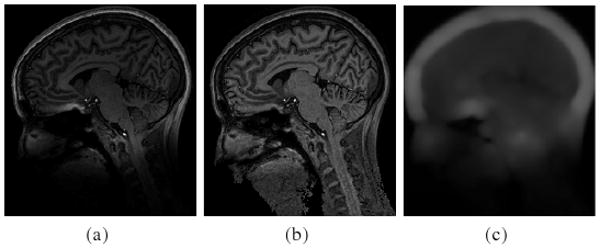
Application of our method to a 7T MR image. (a) Original image; (b) Bias corrected image; (c) Computed bias field.

In this paper, we propose a variational level set approach to bias correction and segmentation for images corrupted with intensity inhomogeneities. A unique feature of our method is that the computed bias field is intrinsically ensured to be smooth by the data term in our variational formulation, without any additional effort to maintain the smoothness of the bias field, and it can approximate bias fields of more general profiles, such as those in 7T MR images. Moreover, our method is not sensitive to initialization, thereby allowing automatic applications.

2 Method

2.1 Model of Images with Intensity Inhomogeneity

Our method is based on the model commonly used to describe images with intensity inhomogeneity:

$$I=\stackrel{\sim }{b}\stackrel{\sim }{J}+n$$ (1)

where I is the measured image intensity, J̃ is the true signal to be restored, b̃ is the bias field, and n is noise. The superscript tilde in J̃ and b̃ is used to distinguish the unknown true signal J̃ and the bias field b̃ from their estimates, which will be denoted by J and b, respectively. The generally accepted assumption on the bias field is that it is smooth (or slowly varying). Ideally, the intensity J̃ in each tissue should take a specific value c̃_i of the physical property being measured (e.g. the proton density for MR images).

In general, we assume that the true image J̃ and the bias field b̃ have the following properties:

(P1) The bias field b̃ is slowly varying in the entire image domain.

(P2) The true image intensities J̃ are approximately a constant within each class of tissue, i.e. J̃(x) ≈ c̃_i for (x) ∈ Ω̃_i, with ${\left\{{\stackrel{\sim }{\Omega }}_i\right\}}_{i=1}^N$ being a partition of Ω.

2.2 Energy Formulation

Our ultimate goal is to separate the image domain Ω into N disjoint regions Ω̃_i, i = 1, ⋯, N, based on the measured image I. However, due to the intensity inhomogeneity caused by the bias field b̃, the measured intensities are not separable by using traditional intensity based classification methods. In this section, we will propose a new method for joint segmentation and bias correction. Our method is based on an observation that the intensities in a relatively small region are separable, which can be verified by the above assumptions (P1) and (P2) as explained in the following.

We consider a circular neighborhood with a relatively small radius ρ centered at each point x in the image domain Ω, defined by $O_{\text{x}}\stackrel{\Delta }{=}\{y:|y-x|\le \rho \}$. The partition ${\left\{{\stackrel{\sim }{\Omega }}_i\right\}}_{i=1}^N$ induces a partition of the neighborhood O_x, i.e., ${\left\{O_x\cap {\stackrel{\sim }{\Omega }}_i\right\}}_{i=1}^N$. For a smooth function b̃, the values b̃(y) for all y in the circular neighborhood O_x can be well approximated by b̃(x), which is at the center of O_x. Therefore, the intensities b̃(y)J̃(y) in each subregion O_x ∩ Ω̃_i are approximately the constant b(x)c̃_i. Thus, we have the following approximation

$$\begin{array}{cc}\stackrel{\sim }{b}(y)\stackrel{\sim }{J}(y)\approx \stackrel{\sim }{b}(x){\stackrel{\sim }{c}}_i& \text{for}y\in O_x\cap {\stackrel{\sim }{\Omega }}_i\end{array}$$ (2)

The constants b̃(x)c̃_i can be considered as the approximations of the cluster centers (or means) of the clusters {I(y) : y ∈ O_x ∩ Ω̃_i} within the neighborhood O_x. Therefore, the intensities in the neighborhood O_x are around N distinct cluster centers m̃_i ≈ b̃(x)c̃_i. The multiplicative components b(x) and c̃_i of the cluster centers m̃_i ≈ b̃(x)c̃_i can be estimated as the following.

Consider the task of classifying the intensities I(y) in the neighborhood O_x into N classes. In view of the separability of the intensities within the neighborhood O_x, this task can be performed by using the standard K-means clustering method. In this paper, we introduce a K-means clustering method based on the minimization of the following weighted objective function

$${\epsilon }_x=\sum _{i=1}^N{\int }_{O_x\cap {\Omega }_i}K(x-y)|I(y)-b(x)c_i{|}^{2}dy$$ (3)

where b(x)c_i are the cluster centers to be optimized, and K(x − y) is a non-negative weighting function such that K(x − y) = 0 for |x − y| > ρ and ∫_Ox K(x − y)dy = 1. Although the choice of the weighting function is flexible, it is preferable to use a weighting function K(x − y) such that larger weights are assigned to the data I(y) for y closer to the center x of the neighborhood O_x. In this paper, the weighting function K is chosen as a truncated Gaussian kernel

$$K(u)=\{\begin{array}{cc}\frac{1}{a}{e}^{-|u{|}^2/2{\sigma }^2}& \text{for}|u|\le \rho \\ 0& \text{else}\end{array}$$

where a is a constant such that ∫ K(u) = 1. The above objective function ε_x can be rewritten as

$${\epsilon }_x=\sum _{i=1}^N{\int }_{{\Omega }_i}K(x-y)|I(y)-b(x)c_i{|}^{2}dx$$ (4)

due to the fact that K(x − y) = 0 for y ∉ O_x.

As mentioned above, the measured intensities I(y) within the neighborhood O_x are separable, and therefore could be classified into N clusters by minimizing the objective function ε_x, which results in the optimal cluster centers m_i and an optimal partition of O_x. However, we still cannot determine the components b(x) and c_i of the computed cluster centers m_i. Moreover, our ultimate goal is to find an optimal set of a partition of the entire image domain Ω, the bias field b, and the constants c_i. The minimization of a single objective function ε_x, which is defined for a point x, does not achieve this goal. We need to minimize ε_x for all the points x. This can be achieved by minimizing the integral of ε_x over Ω. Therefore, we define an energy $\epsilon \stackrel{\Delta }{=}\int {\epsilon }_{x}dx$, i.e.

$$\epsilon \stackrel{\Delta }{=}\int \left(\sum _{i=1}^N{\int }_{{\Omega }_i}K(\text{x}-y)|I(y)-b(x)c_i{|}^{2}dy\right)dx$$ (5)

Directly minimizing the energy with the partition ${\left\{{\Omega }_i\right\}}_{i=1}^N$ as a variable is not convenient. We will use one or multiple level set functions to represent a partition ${\left\{{\Omega }_i\right\}}_{i=1}^N$. The energy minimization can thus be performed by solving a level set evolution equation.

3 Level Set Formulation

We first consider the case of N = 2. In this case, the image domain is partitioned into two regions ${\left\{{\Omega }_i\right\}}_{i=1}^2$. These two regions can be represented by the regions separated by the zero level contour of a function φ, i.e., ${\Omega }_1\stackrel{\Delta }{=}\left\{\phi >0\right\}$ and ${\Omega }_2\stackrel{\Delta }{=}\left\{\phi <0\right\}$. Using Heaviside function H, the energy ε in Eq. (5) can be expressed as an energy in terms of φ, b, and c as below

$$\epsilon (\phi ,b,c)=\int \left(\sum _{i=1}^2\int K(x-y)|I(y)-b(x)c_i{|}^2{M}_i(\phi (y))dy\right)dx$$ (6)

where M₁(φ(x)) = H(φ(x)) and M₂(φ(x)) = 1 − H(φ(x)). In practice, we use a smoothed Heaviside function $H_{\epsilon }(x)=\frac{1}{2}\left[1+\frac{2}{\pi }\text{arctan}\left(\frac{x}{\epsilon }\right)\right]$ to approximate the original Heaviside function H, with ε = 1 as used in [11].

It is necessary to add a regularization term R(φ) to the above energy in the following energy functional:

$$F(\phi ,b,c_1,c_2)\stackrel{\Delta }{=}\epsilon (\phi ,b,c)+R(\phi )$$ (7)

where $R(\phi )\stackrel{\Delta }{=}\nu \int |\nabla H(\phi )|dx+\mu \int {(|\nabla \phi |-1)}^{2}dx$. The first term in R serves to regularize the zero level contour of φ as in typical level set methods [11], while the second term regularizes the entire level set function φ by penalizing its deviation from signed distance, as in the level set methods proposed by Li et al. [12,13]. The energy ε(φ, b, c) is the data term in our variational framework.

Similarly, we can use multiple level set functions φ₁, ⋯, φ_n to represent regions ${\left\{{\Omega }_i\right\}}_{i=1}^N$ with N = 2ⁿ as in [14]. For convenience, we use a vector valued function Φ = (φ₁, ⋯, φ_n) to represent the functions φ₁, ⋯, φ_n. The energy for general multiphase formulation of our method can be defined as

$$F(\Phi ,b,c)\stackrel{\Delta }{=}\int (\text{∑}_{i=1}^N\int K(x-y)|I(y)-b(x)c_i{|}^2{M}_i(\Phi (y))dy)dx+\text{∑}_{i=1}^{n}R({\phi }_i)$$ (8)

where M_i(Φ) are functions of Φ which are designed such that ${\sum }_{i=1}^N{M}_i(\Phi )=1$. The definition of M_i in the four-phase case are given in [14]. For N = 3 and two level set functions φ₁ and φ₂, we can define M₁(φ₁, φ₂) = H(φ₁)H(φ₂), M₂(φ₁, φ₂) = H(φ₁)(1 − H(φ₂)), and M₃(φ₁, φ₂) = 1 − H(φ₁) to obtain a three-phase formulation.

We only describe the energy minimization for the two-phase case in this paper (the multi-phase case can be solved with the similar procedure). For fixed c and b, the minimization of F(φ, c, b) consists in solving the level set evolution equation as the gradient descent equation

$$\frac{\partial \phi }{\partial t}=-\frac{\partial F}{\partial \phi }$$ (9)

where $\frac{\partial F}{\partial \phi }$ is the Gâteaux derivative (the first order functional derivative) of the energy F. In numerical implementation, at each iteration according to Eq. (9), the variables c and b are updated according to the following procedure. For fixed φ and c, we find an optimal bias field b̂ that minimizes F(φ, c, b). It can be shown that the minimizer b̂ is

$$\widehat{b}=\frac{(I{J}^{(1)})\ast K}{J^{(2)}\ast K}$$ (10)

where * is the convolution operation, and $J^{(1)}={\sum }_{i=1}^N{c}_i{M}_i(\phi )$ and $J^{(2)}={\sum }_{i=1}^N{c}_i^2{M}_i(\phi )$. For fixed φ and b, we find an optimal ĉ that minimizes F(φ, c, b). By some calculus manipulations, it can be shown that the minimizer ĉ = (ĉ_i, ⋯, ĉ_N) is

$$\begin{array}{cc}{\widehat{c}}_i=\frac{\int (b\ast K)I{M}_i(\phi )dx}{\int (b^2\ast K)M_i(\phi )dx},& i=1,\cdots ,N.\end{array}$$ (11)

It is worth noting that the expression of b̂ in Eq. (10) with convolutions shows that b̂ is smooth. The smoothness of b̂ is intrinsically ensured by the data term ε(φ, c, b) in our variational framework. This is a desirable advantage of our method: there is no need for imposing a smoothing term to ensure the smoothness of the bias field.

4 Experimental Results and Validation

We use the parameters σ = 4, μ = 1, and ν = 0.001 × 255² for all the images in this paper. Our method is robust to the initialization of the constants c = (c₁, ⋯, c_N), the bias field b, and the level set functions. For automatic applications, the constants c₁, ⋯, c_N can be initialized as N equally spaced numbers between the minimum and maximum intensities of the original image, and the bias field b is initialized as b = 1. The level set functions can be automatically generated or manually initialized by the users. The number of phases N depends on the number of tissue types in the images, which is usually known in practice.

We first demonstrate our method in the two-phase case (i.e. N = 2). For example, Fig. 1 shows the result of our method for an X-ray image. Intensity inhomogeneity is obvious in this image. We use this example to show the desirable capability of our method in joint segmentation and bias correction. The bias corrected image is given by the quotient I/b̂. It is worth noting that our method allows for flexible initialization of the level set function. The initial contour can be inside, outside, or cross the object boundaries. This can be seen from the results in Fig. 1 and those for a computed tomography angiography (CTA) image of vessel and a computed tomography (CT) image of a tumor in a liver shown in Fig. 2. The initial contours used to generate the initial level set functions are shown in Fig. 2(a) and 2(c), and the corresponding segmentation results are shown in Fig. 2(b) and 2(d).

Fig. 1.

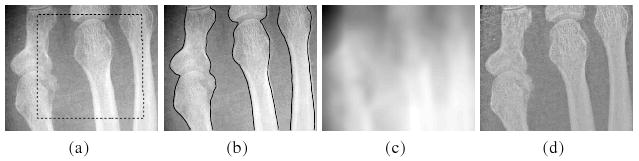
Applications of our method to an X-ray image. (a) Original image and initial contour (dashed black line); (b) Segmentation result (black lines); (c) Computed bias field; (d) Bias corrected image.

Fig. 2.

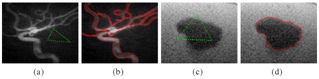
Applications of our method to a CTA image and a CT image. (a) Original CTA image and initial contour (green dashed line); (b) Segmentation result; (c) Original CT image and initial contour; (d) Segmentation result.

Fig. 3 shows the result for a 3T MR brain image, which has obvious intensity inhomogeneity. The computed bias field and the segmentation result are simultaneously obtained, shown in Fig. 3(c) and 3(b), respectively. The bias corrected image is shown in Fig. 3(d). For comparison with other methods, we use coefficient of variance (CV) as a metric to evaluate the performance of the algorithms for bias correction and segmentation (c.f. [9,7]). Coefficient of variance is defined as a quotient between standard deviation and mean value of selected tissue class. A good algorithm for bias correction and segmentation should give low CV values for the bias corrected intensities within each segmented region. We tested our method and the methods of Leemput et al. and Wells et al. with two simulated images obtained from BrainWeb in the link http://www.bic.mni.mcgill.ca/brainweb/, one corrupted with bias field without noise and the other corrupted with both bias and noise. The CV values for the two images are listed in Table 1. It can be seen that the CV values of our method are lower than those of Leemput's and Wells's methods, which indicates that the bias corrected images obtained in our method are more homogeneous than those of the other two methods. In Fig. 4, we show the bias corrected images for the noisy image as an example.

Fig. 3.

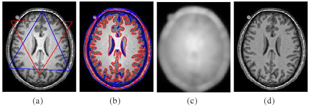
Applications of our method to a 3T MR image. (a) Original image and initial contours: zero level contours of initial φ₁ (red) and φ₂ (blue). (b) Final zero level contours of φ₁ (red) and φ₂ (blue); (c) Computed bias field; (d) Bias corrected image.

Table 1.

Coefficient of Variation

	Tissue	original	Bias corrected
			Wells	Leemput	Our method
Image with bias	WM	20.16%	6.33%	6.81%	5.48%
	GM	23.65%	16.11%	16.97%	14.38%
Image with bias and noise	WM	18.93%	6.97%	7.92%	6.77%
	GM	21.20%	13.65%	14.68%	12.81%

Fig. 4.

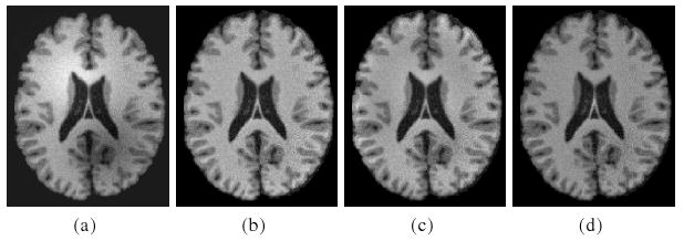
Comparison with the methods of Wells et al. and Leemput et al. using simulated data obtained from BrainWeb. (a) Original image; (b) Our method; (c) Leemput et al.; (d) Wells et al..

Our method has been tested on 7T MR images. At 7T, significant gains in image resolution can be obtained due to the increase in signal-to-noise ratio. However, susceptibility-induced gradients scale with main field, while the imaging gradients are currently limited to essentially the same strengths as used at lower field strengths (i.e., 3T). Such effects are most pronounced at air/tissue interfaces, as can be seen in Fig. 5(a) at the base of the frontal lobe. This appears as a localized and stronger bias, which is challenging to traditional methods for bias correction. This result shows the ability of our method to capture and correct such bias, as shown in Fig. 5(b) and 5(c).

5 Conclusion

We have presented a unified framework of bias correction and segmentation. A unique advantage of our method is that the smoothness of the computed bias field is intrinsically ensured by the data term in our variational formulation. Our method is able to capture bias of quite general profiles, and can be used for images of various modalities. Moreover, it is robust to initialization, thereby allowing automatic applications. Comparisons with two well-known bias correction methods demonstrate the advantages of the proposed method.

References

- 1.Wells W, Grimson E, Kikinis R, Jolesz F. Adaptive segmentation of MRI data. IEEE Trans Med Imag. 1996;15(4):429–442. doi: 10.1109/42.511747. [DOI] [PubMed] [Google Scholar]
- 2.Vovk U, Pernus F, Likar B. A review of methods for correction of intensity inhomogeneity in mri. IEEE Trans Med Imag. 2007;26(3):405–421. doi: 10.1109/TMI.2006.891486. [DOI] [PubMed] [Google Scholar]
- 3.Lewis E, Fox N. Correction of differential intensity inhomogeneity in longitudinal MR images. Neuro image. 2004;23(3):75–83. doi: 10.1016/j.neuroimage.2004.04.030. [DOI] [PubMed] [Google Scholar]
- 4.Dawant B, Zijdenbos A, Margolin R. Correction of intensity variations in MR images for computer-aided tissues classification. IEEE Trans Med Imag. 1993;12(4):770–781. doi: 10.1109/42.251128. [DOI] [PubMed] [Google Scholar]
- 5.Meyer C, Bland P, Pipe J. Retrospective correction of intensity inhomogeneities in MRI. IEEE Trans Med Imag. 1995;14(1):36. doi: 10.1109/42.370400. [DOI] [PubMed] [Google Scholar]
- 6.Sled J, Zijdenbos A, Evans A. A nonparametric method for automatic correction of intensity nonuniformity in MRI data. IEEE Trans Med Imaging. 1998;17(1):87–97. doi: 10.1109/42.668698. [DOI] [PubMed] [Google Scholar]
- 7.Leemput K, Maes F, Vandermeulen D, Suetens P. Automated model-based bias field correction of MR images of the brain. IEEE Trans Med Imag. 1999;18(10):885–896. doi: 10.1109/42.811268. [DOI] [PubMed] [Google Scholar]
- 8.Styner M, Brechbuhler C, Szekely G, Gerig G. Parametric estimate of intensity inhomogeneities applied to MRI. IEEE Trans Med Imag. 2000;19(3):153–165. doi: 10.1109/42.845174. [DOI] [PubMed] [Google Scholar]
- 9.Guillemaud R, Brady M. Estimating the bias field of MR images. IEEE Trans Med Imaging. 1997;16:238–251. doi: 10.1109/42.585758. [DOI] [PubMed] [Google Scholar]
- 10.Pham D, Prince J. Adaptive fuzzy segmentation of magnetic resonance images. IEEE Trans Med Imag. 1999;18(9):737–752. doi: 10.1109/42.802752. [DOI] [PubMed] [Google Scholar]
- 11.Chan T, Vese L. Active contours without edges. IEEE Trans Imag Proc. 2001;10:266–277. doi: 10.1109/83.902291. [DOI] [PubMed] [Google Scholar]
- 12.Xu C, Li C, C G, Fox MD. Level set evolution without re-initialization: A new variational formulation. IEEE Conference on Computer Vision and Pattern Recognition (CVPR); 2005. pp. 430–436. [Google Scholar]
- 13.Li C, Kao C, Gore J, Ding Z. Implicit active contours driven by local binary fitting energy. IEEE Conference on Computer Vision and Pattern Recognition (CVPR); 2007. [Google Scholar]
- 14.Vese L, Chan T. A multiphase level set framework for image segmentation using the mumford and shah model. Int'l J Comp Vis. 2002;50:271–293. [Google Scholar]