Global sea level linked to global temperature

Abstract

We propose a simple relationship linking global sea-level variations on time scales of decades to centuries to global mean temperature. This relationship is tested on synthetic data from a global climate model for the past millennium and the next century. When applied to observed data of sea level and temperature for 1880–2000, and taking into account known anthropogenic hydrologic contributions to sea level, the correlation is >0.99, explaining 98% of the variance. For future global temperature scenarios of the Intergovernmental Panel on Climate Change's Fourth Assessment Report, the relationship projects a sea-level rise ranging from 75 to 190 cm for the period 1990–2100.

Sea-level rise is among the potentially most serious impacts of climate change. But sea-level changes cannot yet be predicted with confidence using models based on physical processes, because the dynamics of ice sheets and glaciers and to a lesser extent that of oceanic heat uptake is not sufficiently understood. This limited understanding is seen, e.g., in the fact that observed sea-level rise exceeded that predicted by models (best estimates) by ≈50% for the periods 1990–2006 (1) and 1961–2003 (2). The last Intergovernmental Panel on Climate Change (IPCC) assessment report did not include rapid ice flow changes in its projected sea-level ranges, arguing that they could not yet be modeled, and consequently did not present an upper limit of the expected rise (2).

This problem has caused considerable recent interest in semiempirical approaches to projecting sea-level rise (3–8). These approaches are based on using an observable that climate models actually can predict with confidence, namely global mean temperature, and establish with the help of observational data how global mean temperature is linked to sea level. A limitation of this approach is that a response that differs fundamentally from that found in the data used cannot be captured, for example, a large and highly nonlinear ice discharge event of a type not in the observational record. This limitation has to be kept in mind when interpreting the results. Here, we present a substantial extension and improvement to the semiempirical method proposed by Rahmstorf (3) (henceforth called R07). We test it on synthetic and real data and apply it to obtain revised sea-level projections up to the year 2100.

Model

Rahmstorf (3) originally proposed that the initial rate of sea-level rise in response to a large, rapid warming could be approximated by

Here, T₀ is a base temperature at which sea level is in equilibrium with climate, so that the rate of rise of sea level H, dH/dt, is proportional to the warming above this base temperature. T₀ and a are to be determined from data. For the ice-melt contribution (glaciers and ice sheets) this approach corresponds to one commonly used in ice modeling, where the rate of mass loss is assumed to be proportional to the temperature increase above a threshold value (9). Some statistical aspects of this work were subsequently challenged (10, 11), but in response the results were shown to be robust with respect to various choices in the analysis method (12).

Eq. 1 is based on the assumption that the response time scale τ of sea level is long compared with the time scale of interest (typically ≈100 years). Grinsted et al. (8) have recently proposed to model the link of sea level and temperature with a single finite time scale. For the fit to instrumental temperature and sea-level data they obtain a time scale of just over 1,000 years, thus essentially replicating the results of R07, albeit with a different sea-level dataset. However, some components of sea level adjust quickly to a temperature change, e.g., the heat content of the oceanic surface mixed layer. Therefore, we here propose to extend the semiempirical method by a rapid-response term:

This second term corresponds to a sea-level response that can be regarded as “instantaneous” on the time scales under consideration, because it implies H ∼ T. Given the two time scales represented, we will call this the dual model.

Results

Testing the Dual Model on Simulated Future Sea-Level Rise.

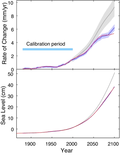
Testing analysis methods by applying them to model-generated data in addition to those from the real world is a widely used approach. A key advantage of this method is that in the model world, we have complete information and can also analyze future high-CO₂ scenarios. R07 presented a test of his method on future sea-level projections from a coupled climate model (13) and found the method was unable to capture a leveling off of the rate of sea-level rise in the second half of the 21st century found in the climate simulation. We repeat this test with the dual model (Fig. 1). The parameters are fitted to the global temperature and sea-level output from the climate model for 1880–2000, resulting in a = 0.080 ± 0.017 cm·K⁻¹·a⁻¹, b = 2.5 ± 0.5 cm·K⁻¹, and T₀ = −0.375 ± 0.026 K (temperature relative to the reference period 1951–1980). Sea level for 2000–2100 is then computed from global temperature using Eq. 2 and compared with the sea level simulated by the climate model (which includes a 3D ocean general circulation model) (13). The fact that the rate of rise levels off after 2050 is captured well by the dual model, a circumstance related to temperatures rising less than exponentially. As seen from Eqs. 1 and 2, the dual model is equivalent to the R07 model in case of an exponential temperature increase.

Fig. 1.

The 21st-century simulation. (Upper) The rate of sea-level rise from a climate model simulation (red) compared with that predicted by Eq. 1 (gray) and Eq. 2 (blue) based on global mean temperature from the climate model. Shaded areas show the uncertainty of the fit (1 SD). The parameter calibration period is 1880–2000, and 2000–2100 is the validation period. (Lower) The integral of the curves in Upper, i.e., sea-level proper.

Note that this test is for the thermal expansion component of sea-level rise only, because only that is captured in the climate model. In this case, we expect the rapid response of sea level (second term) to be caused by heat uptake of the surface mixed layer of the ocean, for which ΔH = h·α· ΔT, where h is the mixed layer depth and α is the mean thermal expansion coefficient. Hence, b = h·α. For a typical value α = 2.5 × 10⁻⁴ K⁻¹ (sea water at 20 °C), the value we found for b corresponds to a mixed layer depth of h = 100 m. This physically plausible result is evidence for the validity of the method.

Testing the Dual Model for the Past Millennium.

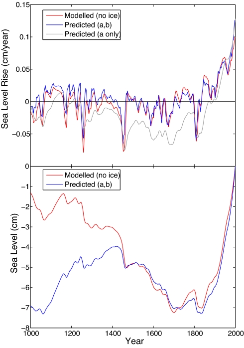
The model of R07 was criticized for not performing well in a model test under conditions of past natural variability, dominated by the response to volcanic eruptions (6). Although R07 by design was not applicable to such conditions, it makes sense to perform such a test on the dual model. For this test we used a model simulation of the past millennium, where the climate model was forced by solar variability, volcanic activity, changes in greenhouse gas concentration, and tropospheric sulfate aerosols. This simulation, along with the forcing and a range of other models, was published in the IPCC Fourth Assessment Report (2) (AR4; figure 6.14 thereof) and compared with paleo-climatic data. We applied the dual model fit discussed in the previous section, using parameters a and b obtained there to predict sea-level variations for the time period 1000 to 2000 AD (Fig. 2). A small adjustment was applied visually to T₀ to make long-term sea-level rise match; any small error in this parameter would lead to a drift in sea level that accumulates over time and becomes an issue over multiple centuries.

Fig. 2.

The millennnium simulation. (Upper) Rate of sea-level rise for the last millennium from a climate model simulation (red), compared with that predicted by Eq. 1 (gray) and Eq. 2 (blue) based on global mean temperature from the climate model. Note that parameter calibration was done for the model simulation shown in Fig. 1 for 1880–2000 only (but see below for T₀). (Lower) Sea level for the last millennium, obtained by integration. A correction to the T₀ parameter of −0.13 K (corresponding to a constant sea-level trend of a·T₀ = −0.1 mm/year) was applied to make the long-term sea-level trends match better after the year 1400.

Fig. 2 shows that the single-term model of R07 can capture the 20th-century sea-level rise but not the short-term variability. The latter is to be expected because basic assumptions behind this approximation are not fulfilled here; the method is used outside of its range of applicability. In contrast, the dual model also captures the short-term response and performs well when compared with the sea-level variations simulated by the climate model, explaining 82% of sea-level rate variance. Even the brief negative excursions of the rate of sea-level change caused by volcanic eruptions (which in this model are implemented as a globally averaged forcing) are reproduced faithfully. A mismatch in Fig. 2 Lower in the first few centuries is caused by a small offset in the rate there; adjusting T₀ can remove this offset either for the first or the second half of the millennium, but not both. This points to an inherent limitation of assuming an infinite adjustment time scale in the slow term, an assumption that breaks down beyond ≈500 years. This limitation does not affect our fit to the instrumental data and the future projections discussed later, both of which are limited to the 100-year time frame. A good performance is also found for millennial simulations with two other climate models, the ECHO-G model (6) and the ECBilt-CLIO model (14) (see S3 and S4 in SI Appendix).

Testing the Dual Model on Observed Data.

The third and most interesting test is the application to observed data of global temperature and sea level for 1880–2000, because it covers the full climate-related sea-level response and not just thermal expansion. The IPCC AR4 (2) concludes that thermal expansion can explain ≈25% of observed sea-level rise for 1961–2003 and 50% for 1993–2003, but with considerable uncertainty. The remainder is mostly caused by ice melt; climate-induced changes in land water storage played a minor, but not negligible, role (15). A recent analysis concludes that during 2003–2008 the split was 20% thermal and 80% ice melt (16). While a 5-year period is likely to be dominated by natural variability, there is some reason for concern that ice melt could take an increasingly larger share in the course of this century.

For temperature we use the National Aeronautics and Space Administration's Goddard Institute for Space Studies dataset (17) because it has the best global coverage. For sea level we use the data of Church and White (18) as adopted by the IPCC. These sea-level data are already corrected for postglacial rebound; because this is a constant linear trend it does not affect our proposed link to temperature. We further corrected the sea-level data for the amount of water stored in manmade reservoirs (see SI Appendix), because they cause a small sea-level drop not related to climate that must be excluded from the sea-level changes linked to global temperature as considered in Eq. 2. Possible effects of groundwater mining are considered below.

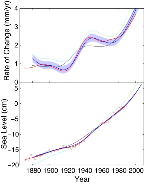
Fig. 3 shows the remarkably close link of global temperature and the rate of sea-level rise we find for 1880–2000. In particular, it shows that the rate of sea-level rise increased up to 1940 in line with rising temperatures, then stagnated up to the late 1970s while global temperature also remained nearly level, followed by another rise that continues until today. Note that the parameters a and T₀ are essentially determined by making mean value and trend agree over the data period. Any agreement of the R07 model (Fig. 3, gray line) with observed sea level beyond the linear trend is thus not fitted but an independent test of the concept. The near-perfect fit of the dual model arises because almost all of the remaining misfit of the R07 model is proportional to dT/dt.

Fig. 3.

The duel model in the instrumental period. (Upper) Observations-based rate of sea-level rise (with tectonic and reservoir effects removed; red) compared with that predicted by Eq. 1 (gray) and Eq. 2 (blue with uncertainty estimate) using observed global mean temperature data. Also shown is the estimate from Eq. 2 using only the first half of the data (green) or the second half of the data (light blue). (Lower) The integral of the curves in Upper, i.e., sea-level proper. In addition to the smoothed sea level used in the calculations, the annual sea-level values (thin red line) are also shown. The dark blue prediction by Eq. 2 almost obscures the observed sea level because of the close match.

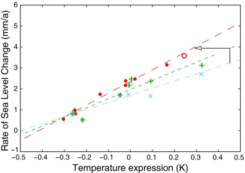
Fig. 4 shows the observations-based rate of sea-level rise as a function of the right sides of Eqs. 1 and 2. The parameter values obtained are T₀ = −0.41 ± 0.03 K, a = 0.56 ± 0.05 cm·a⁻¹·K⁻¹, and b = −4.9 ± 1.0 cm·K⁻¹. The linear fit is clearly better for the dual model: the Pearson correlation coefficient r = 0.992 for the dual model (0.96 for the R07 model even when the artificial reservoir correction is applied). This finding is to be expected because the model contains one additional free parameter. Whether it still is the preferred model when this extra degree of freedom is taken into account can be tested with the Akaike information criterion, a standard statistical technique for such cases (see SI Appendix). The analysis shows that the dual model is the preferred model, suggesting also here that the second term is physically meaningful.

Fig. 4.

Blue crosses show 15-year averages of global temperature (relative to 1951–1980) versus the rate of sea-level rise, with their linear least-squares fit, as in R07 (3) but using 15-year bins. The green crosses show the adjustment to sea level induced by the reservoir correction (22), leading to a steeper slope. The red dots show the expression (T + b/a dT/dt) appearing on the right of Eq. 2. This increases the slope again and leads to a much tighter linear fit. The open red circle is a data point based on the satellite altimetry data for 1993–2008. The arrow indicates how the linear trend line changes from that of R07 (blue) to the green one by adjusting the sea-level data (a change along the vertical axis) and then again to the red line by adjusting the temperature expression (along the horizontal axis).

Another semiindependent test is provided by the satellite sea-level record updated from ref. 16 that started in 1993 and now provides 16 years of data (up including 2008), with a linear trend of 3.4 mm/year (after postglacial rebound adjustment). When the reservoir correction is applied it yields 3.6 mm/year, and the extra point is shown as an open circle in Fig. 4.

Remarkably, the value we find for b is negative. We can think of two possible physical explanations. The first is that the initial rapid sea-level response to a warming is indeed negative. A possible mechanism for this is higher evaporation from the sea surface and subsequent storage of extra water on land, e.g., in form of soil moisture (19, 20). Note, however, that such a negative effect would have to be large: it would need to compensate the b of +2.5 cm·K⁻¹ found earlier for thermal expansion and thus would need to be three times as large as this to cause the overall negative b value we found. It is hard to see how the very large amount of water needed to be stored on land could remain inconspicuous.

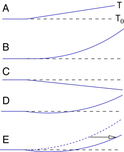
The second possibility is of a positive, but time-lagged, sea-level response. That a negative b corresponds to a lag is easily seen for the example of a steady linear temperature rise with rate c starting at time t = 0. The solution then is H = 1/2 a c t(t + 2b/a). This is the same parabola as for the R07 model (H = 1/2 a c t²), except that its origin is shifted by (b/a, b²c/2a) (see Fig. 5). For c = 0.01 K·a⁻¹ (i.e., an idealized 20th-century warming) and the parameter values found above, this shift is 12 years and −0.25 cm. The short transient sea-level offset of a maximum of −2.5 mm is too small to measure and of no consequence on the longer time scales (>15 years) considered here. However, the implied time lag of 12 years in this idealized case is permanent and significant.

Fig. 5.

Schematic of the response to a linear temperature rise. (A) Temperature. (B) First term on the right of Eq. 2. (C) Second term. (D) Total sea-level response. (E) Comparison to the case b = 0 (Eq. 1), showing that b < 0 primarily corresponds to a time lag in the sea-level response.

We tested this idea by implementing a time lag directly in Eq. 2:

and subsequently finding the best fit for T₀, a, b, and τ. When the resulting Pearson correlation is plotted as a function of b and τ (see Fig. 2), a linear dependence between the two is seen, with two optimal solutions: one for zero τ and b = −5 cm·K⁻¹, and another one b = 4.5 cm·K⁻¹ and τ = 13 years. Choosing the value b = 2.5 cm·K⁻¹ from our model simulations for the thermal expansion effect corresponds to τ = −11 years, close to this optimum. The two parameters b and τ cannot be unambiguously separated by the statistical fit because their effect on H is so similar. Thus, the most plausible physical interpretation of our statistical fit is that the negative value of b results from a positive ocean mixed layer response combined with a lag of over a decade in the response of the ocean-cryosphere system.

Several mechanisms could be envisaged for a delayed onset of sea-level rise after warming. For example, mass loss of ice sheets can be caused by warm water penetrating underneath ice shelves, triggering their collapse and subsequent speed-up of outlet glaciers banked up behind the ice shelf (21). We cannot explore the causes of delay in more detail here, but note that the statistical result is robust irrespective of its causes.

The quality of fit found also independently confirms the quality on interdecadal time scales of both the global temperature and sea-level time series used. Any erroneous long-term trend in temperatures or acceleration in sea level would cause conspicuous misfits. The reservoir adjustment (22) is a major contributor to the success of the fit. Given that the reservoir adjustment is a known and valid correction this further corroborates the physical basis of the agreement we find.

Other Nonclimatic Sea-Level Contributions.

We have corrected the sea-level data for the reservoir storage component, but a further nonclimatic effect of relevant magnitude is the mining of groundwater for human uses in arid regions (23). No time series of this is available, so it cannot be included in the above analysis. We consider it an uncertainty and test the sensitivity of our results to this term.

Estimates differ considerably, but in recent decades groundwater mining could have contributed 0.2–0.3 mm/year to sea level (23). We consider two scenarios for the time evolution leading up to this high-end estimate: a linear and an exponential increase of the pumping rate, starting at zero in the year 1870 (see SI Appendix). Remarkably and contrary to the reservoir storage correction, neither scenario significantly affects the quality of fit found. For all cases, fit parameters remain within the 1σ uncertainty of their values found in the previous section. The temperature sensitivity of long-term sea-level change a is reduced by 6–7%. The impact on future sea-level projections is reduced by the fact that groundwater mining for irrigation purposes is likely to increase in the future and in this sense behaves like the climate-related component of sea-level rise. This behavior is in contrast to that of the reservoir correction included above, because the potential for additional water storage on land is limited and reservoir building has declined and almost come to an end (22).

Projections of Future Sea Level.

After Eq. 2 has passed a 3-fold test with simulated and observed sea-level data, we will apply it to the 21st century by using global temperature projections from the IPCC AR4 (2). We use the emulated global temperature data for 1880–2100 for six emission scenarios, three carbon cycle feedback scenarios, and 19 climate models, as shown in figure 10.26 of the AR4 (2). For these 342 temperature scenarios sea level was computed by using Eq. 2, assuming equal average temperatures across all models for the period 1880–1920, close to preindustrial temperatures. This reference period leads to slightly different temperatures (and hence rates of sea-level rise) in 1990 according to the climate sensitivity of the respective model; more sensitive models show greater warming and greater sea-level rise consistently for the 20th and 21st centuries.

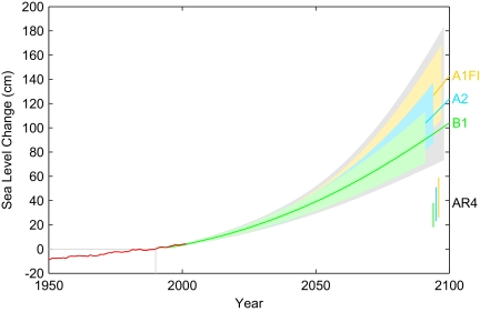
For each of the six emission scenarios, we computed the mean sea-level curve across all 19 models, using the standard carbon cycle setting. These are the solid lines shown in Fig. 6 for three of the emissions scenarios. The colored uncertainty bands for each scenario encompass 1 SD from the model mean, using the high carbon cycle setting for the upper uncertainty limit and the low carbon cycle setting for the lower limit, as is done in the AR4 (2) for temperatures. The additional gray uncertainty band shows an added ± 7%, representing 1 SD of the uncertainty of the fit shown in Fig. 4. The temperature and sea-level ranges for all six emission scenarios are compiled in Table 1.

Fig. 6.

Projection of sea-level rise from 1990 to 2100, based on IPCC temperature projections for three different emission scenarios (labeled on right, see Projections of Future Sea Level for explanation of uncertainty ranges). The sea-level range projected in the IPCC AR4 (2) for these scenarios is shown for comparison in the bars on the bottom right. Also shown is the observations-based annual global sea-level data (18) (red) including artificial reservoir correction (22).

Table 1.

Temperature ranges and associated sea-level ranges by the year 2100 for different IPCC emission scenarios

Scenario	Temperature range,°C above 1980–2000	Model average,°C above 1980–2000	Sea-level range,cm above 1990	Model average,cm above 1990
B1	1.4–2.9	2.0	81–131	104
A1T	1.9–3.8	2.6	97–158	124
B2	2.0–3.8	2.7	89–145	114
A1B	2.3–4.3	3.1	97–156	124
A2	2.9–5.3	3.9	98–155	124
A1FI	3.4–6.1	4.6	113–179	143

The temperatures used are taken from the simple model emulation of 19 climate models as shown in figure 10.26 of the IPCC AR4 (2); they represent the mean ± 1 SD across all models, including carbon cycle uncertainty. The sea-level estimates were produced by using Eq. 2 and 342 temperature scenarios and are given here excluding the uncertainty of the statistical fit, which is approximately ± 7% (1 SD).

Overall, sea-level projections range from 75 to 190 cm for the period 1990–2100. In the two sensitivity scenarios for groundwater mining discussed above, the lowest climate-related sea level rise drops from 81 cm (see Table 1) to 75–76 cm. However, as mentioned above, groundwater mining will continue to raise sea level. Even without further increase, i.e., at a constant mining rate of 0.3 mm/year, this would add 3.3 cm to the projection, increasing it to 78–79 cm. Hence, even considering high-end estimates for the effect of past groundwater mining all scenarios remain well within the overall range shown in Fig. 6.

The model averages for all emission scenarios are remarkably close together, mostly because sea-level rise integrates the temperature rise over time in the first term of Eq. 2, so that a temperature increment in 1999 has 100 times the effect on final sea level compared with the same increment in 2099. Temperatures in the various emission scenarios are still close together in the first half of the century. The second term in Eq. 2 furthermore implies a time lag, so that emissions reductions (as in scenario B1) only slow down sea-level rise after more than a decade delay. These results suggest that emissions reductions early in this century will be much more effective in limiting sea-level rise than reductions later on. This effect can be seen when comparing scenarios A1B and A2, which produce the same sea-level rise by 2100 despite A1B being 0.8 °C cooler then. This result is caused by A1B being slightly warmer early on in the 21st century.

Another interesting aspect of these projections is that the thermal share in the rate of sea-level rise declines over the 21st century, if we take the parameters (a, b) fitted to the climate model simulation above to represent thermal expansion. For the period 1961–2003, the thermal share is ≈30%, as compared with 25% estimated in the AR4 (2) and 40% by Domingues et al. (24). In our projection it gradually declines to ≈20% in the latter half of the 21st century and is directly linked to the fact that thermal expansion is associated with positive b while total sea level has a negative b, corresponding to a delay in the ice response. Qualitatively we consider this decline in the thermal share and increasing importance of ice melt a robust result, which is our key difference to the IPCC AR4 (2), where the ice-melt share is assumed to diminish with thermal expansion contributing between 55% and 70% of the total sea-level rise over the 21st century.

Discussion: Implications for the Future

If our method presents a reasonable approximation of the future sea-level response to global warming, then for a given emission scenario sea level will rise approximately three times as much by 2100 as the projections (excluding rapid ice flow dynamics) of the IPCC AR4 (2) have suggested. Even for the lowest emission scenario (B1), sea-level rise is then likely to be ≈1 m; for the highest, it may even come closer to 2 m.

Uncertainties remain, however. While the thermal expansion response has been tested on simulated data, it is less clear whether the information contained in the 120 years of observational data about the ice response is sufficient to describe the future ice-melt contribution out to the year 2100. The key question then is: will the ice-melt response observed so far, as captured in our dual model, overestimate or underestimate future sea-level rise? On one hand, the surface area of mountain glaciers vulnerable to melting will decrease in future as glaciers disappear. However, more ice higher up in mountains and particularly the big continental ice sheets will increasingly become subject to melting as temperatures warm. The net effect, an increasing or decreasing surface area subject to melting, is not easily determined without detailed regional studies. In addition, highly nonlinear responses of ice flow may become increasingly important during the 21st century. These are likely to make our linear approach an underestimate. Therefore, we have to entertain the possibility that sea level could rise faster still than suggested by the simple projection based on Eq. 2.

How much faster? Pfeffer et al. (25) provided an independent estimate of maximum ice discharge based on geographic constraints on ice flow; they concluded that sea-level rise in the 21st century is very unlikely to exceed 200 cm. If this estimate is correct, a nonlinear dynamical ice-sheet response may not change our estimate upward by very much.

To limit global sea-level rise to a maximum of 1 m in the long run (i.e., beyond 2100), as proposed recently as a policy goal (26), deep emissions reductions will be required. Likely they would have to be deeper than those needed to limit global warming to 2 °C, the policy goal now supported by many countries. Our analysis further suggests that emissions reductions need to come early in this century to be effective.

Software code accompanying this article is available (SI Sea-Level Code).

References

- 1.Rahmstorf S, et al. Recent climate observations compared to projections. Science. 2007;316:709. doi: 10.1126/science.1136843. [DOI] [PubMed] [Google Scholar]
- 2.Solomon S, et al., editors. Intergovernmental Panel on Climate Change. The Fourth Assessment Report of the Intergovernmental Panel on Climate Change. Cambridge UK: Cambridge Univ Press; 2007. [Google Scholar]
- 3.Rahmstorf S. A semiempirical approach to projecting future sea-level rise. Science. 2007;315:368–370. doi: 10.1126/science.1135456. [DOI] [PubMed] [Google Scholar]
- 4.Horton R, et al. Sea-level rise projections for current generation CGCMs based on the semiempirical method. Geophys Res Lett. 2008;35:L02715. [Google Scholar]
- 5.Edwards R. Sea levels: Resolution and uncertainty. Progr Phys Geogr. 2007;31:621–632. [Google Scholar]
- 6.von Storch H, Zorita E, Gonzalez-Rouco JF. Relationship between global mean sea level and global mean temperature in a climate simulation of the past millennium. Ocean Dyn. 2008;58:227–236. [Google Scholar]
- 7.Oppenheimer M, O'Neill BC, Webster M. Negative learning. Clim Change. 2008;89:155–172. [Google Scholar]
- 8.Grinsted A, Moore JC, Jefrejeva S. Reconstructing sea level from paleo and projected temperatures 200 to 2100 AD. Clim Dyn. 2009 10.1007/s00382-008-0507-2. [Google Scholar]
- 9.Oerlemans J, et al. Modeling the response of glaciers to climate warming. Clim Dyn. 1998;14:267–274. [Google Scholar]
- 10.Holgate S, Jevrejeva S, Woodworth P, Brewer S. Comment on “a semiempirical approach to projecting future sea-level rise”. Science. 2007;317:1866b. doi: 10.1126/science.1140942. [DOI] [PubMed] [Google Scholar]
- 11.Schmith T, Johansen S, Thejll P. Comment on “a semiempirical approach to projecting future sea-level rise”. Science. 2007;317:1866c. doi: 10.1126/science.1143286. [DOI] [PubMed] [Google Scholar]
- 12.Rahmstorf S. Response to comments on “a semiempirical approach to projecting future sea-level rise”. Science. 2007;317:1866d. [Google Scholar]
- 13.Montoya M, et al. The Earth system model of intermediate complexity CLIMBER-3α. Part I: Description and performance for present-day conditions. Clim Dyn. 2005;26:237–263. [Google Scholar]
- 14.Goosse H, Renssen H, Timmermann A, Bradley RS. Internal and forced climate variability during the last millennium: A model-data comparison using ensemble simulations. Q Sci Rev. 2005;24:1345–1360. [Google Scholar]
- 15.Ramillien G, et al. Land water storage contribution to sea level from GRACE geoid data over 2003–2006. Global Planetary Change. 2008;60:381–392. [Google Scholar]
- 16.Cazenave A, et al. Sea-level budget over 2003–2008: A reevaluation from GRACE space gravimetry, satellite altimetry, and Argo. Global Planetary Change. 2008;65:83–88. [Google Scholar]
- 17.Hansen J, et al. A closer look at United States and global surface temperature change. J Geophys Res. 2001;106:23947–23963. [Google Scholar]
- 18.Church JA, White NJ. A 20th-century acceleration in global sea-level rise. Geophys Res Lett. 2006;33:L01602. [Google Scholar]
- 19.Chen JL, Wilson CR, Chambers DP, Nerem RS, Tapley BD. Seasonal global water mass budget and mean sea-level variations. Geophys Res Lett. 1998;25:3555–3558. [Google Scholar]
- 20.Ngo-Duc T, Laval K, Polcher J, Lombard A, Cazenave A. Effects of land water storage on global mean sea level over the past half-century. Geophys Res Lett. 2005;32:L09704. [Google Scholar]
- 21.Holland DM, Thomas RH, De Young B, Ribergaard MH, Lyberth B. Acceleration of Jakobshavn Isbrae triggered by warm subsurface ocean waters. Nat Geosci. 2008;1:659–664. [Google Scholar]
- 22.Chao BF, Wu YH, Li YS. Impact of artificial reservoir water impoundment on global sea level. Science. 2008;320:212–214. doi: 10.1126/science.1154580. [DOI] [PubMed] [Google Scholar]
- 23.Milly PCD, et al. In: Church JA, Woodworth P, Aarup T, Wilson S, editors. Proceedings of the WCRP Workshop Understanding Sea-Level Rise and Variability; Oxford: Blackwell; 2009. in press. [Google Scholar]
- 24.Domingues CM, et al. Improved estimates of upper-ocean warming and multidecadal sea-level rise. Nature. 2008;453:1090–1096. doi: 10.1038/nature07080. [DOI] [PubMed] [Google Scholar]
- 25.Pfeffer WT, Harper JT, O'Neel S. Kinematic constraints on glacier contributions to 21st-century sea-level rise. Science. 2008;321:1340–1343. doi: 10.1126/science.1159099. [DOI] [PubMed] [Google Scholar]
- 26.Wissenschaftlicher Beirat Globale Umweltveränderungen. The Future Oceans: Warming Up, Rising High, Turning Sour. Berlin: Wissenschaftlicher Beirat Globale Umweltveränderungen; 2006. [Google Scholar]
Associated Data
This section collects any data citations, data availability statements, or supplementary materials included in this article.