Probabilistic Model of Microbial Cell Growth, Division, and Mortality

Abstract

After a short time interval of length δt during microbial growth, an individual cell can be found to be divided with probability P_d(t)δt, dead with probability P_m(t)δt, or alive but undivided with the probability 1 − [P_d(t) + P_m(t)]δt, where t is time, P_d(t) expresses the probability of division for an individual cell per unit of time, and P_m(t) expresses the probability of mortality per unit of time. These probabilities may change with the state of the population and the habitat's properties and are therefore functions of time. This scenario translates into a model that is presented in stochastic and deterministic versions. The first, a stochastic process model, monitors the fates of individual cells and determines cell numbers. It is particularly suitable for small populations such as those that may exist in the case of casual contamination of a food by a pathogen. The second, which can be regarded as a large-population limit of the stochastic model, is a continuous mathematical expression that describes the population's size as a function of time. It is suitable for large microbial populations such as those present in unprocessed foods. Exponential or logistic growth with or without lag, inactivation with or without a “shoulder,” and transitions between growth and inactivation are all manifestations of the underlying probability structure of the model. With temperature-dependent parameters, the model can be used to simulate nonisothermal growth and inactivation patterns. The same concept applies to other factors that promote or inhibit microorganisms, such as pH and the presence of antimicrobials, etc. With P_d(t) and P_m(t) in the form of logistic functions, the model can simulate all commonly observed growth/mortality patterns. Estimates of the changing probability parameters can be obtained with both the stochastic and deterministic versions of the model, as demonstrated with simulated data.

Continuous growth models.

Most traditional microbial isothermal growth models are based on the assumption that the growth curve has three regions: a lag time, an exponential growth phase, and a stationary phase during which the number of cells remains unchanged (19, 20). The corresponding mathematical models are generally of two types: empirical analytical expressions and rate equations. Among the first type, the most widely known is the Gompertz model (19), one form of which is

(1)

where N(t) is the number of cells in a given volume or mass at time t and A, B, C, and μ are adjustable, temperature-dependent growth parameters.

The second type of isothermal growth model consists of various modified versions of the continuous logistic equation, Verhulst's model (31):

(2)

where r is a temperature-dependent rate constant and N_asympt, commonly but erroneously dubbed N_max, is the asymptotic growth level, representing the carrying capacity of the habitat. The model is based on the assumption that the instantaneous growth rate, dN(t)/dt, of an organism introduced into a closed habitat is proportional to the current population size, N(t), and the fraction of resources still unutilized, 1 − N(t)/N_asympt.

According to equation 2, when t is ∼0 and N(0) is ≪N_asympt, dN(t)/dt is ∼rN(t), i.e., the initial growth is approximately exponential. Therefore, Verhulst's model in its original form is unsuitable for growth curves that exhibit a long lag time, unless the initial growth rate is extremely low. A growth model widely used in food microbiology is a modified version of the logistic equation proposed by Baranyi and Roberts (5):

(3)

where dq(t)/dt equals μ_maxq(t), q(t) being the concentration of limiting substrate and μ_max being the maximum specific growth rate, and m is a constant frequently assumed to have the value of 1.

The term q(t)/[1 + q(t)], which is the same as q₀exp(μ_maxt)/[1+ q₀exp(μ_maxt)], is supposed to account for the physiological state of the population at the time of its introduction into a new habitat. Therefore, the Baranyi-Roberts model implies that there is a universal relationship between the lag time and the maximum growth rate (μ_max), a highly questionable proposition (9, 22, 23). A lag time (t_lag) can, of course, be incorporated into any model by replacing the original term N(t) by N_lag(t), equal to N([t − t_lag]⁺), where (t − t_lag)⁺ is 0 for t of <t_lag and is (t − t_lag) for t of ≥t_lag. Then N_lag(t) equals N(0) for t of <t_lag, after which N_lag(t) develops according to the original model, with the time origin shifted to t_lag, for t of ≥t_lag. Other modifications of the logistic equation, such as that by Fujikawa et al. (15), were intended only to improve the logistic model's fit to experimental growth data. Consequently, the authors made no attempt to assign a mechanistic meaning to the added parameters.

None of the above-mentioned models and their variants can describe situations where cell mortality plays a significant role. This is not a serious handicap in modeling food spoilage, for example, where N(t) is defined as the net number of viable organisms. Thus, even if some cells die out during the exponential phase, their departure will hardly have any practical consequences. This is because most untreated or contaminated foods become inedible or unsafe to eat long before the stationary phase is reached and, therefore, what might happen when the bacterial population starts to die off is of little interest. The situation may be different, however, when pathogens rather than spoilage organisms are involved. In such a case, the pathogen's ability merely to survive in the food may determine the associated health risk.

Both types of traditional models can describe only the sigmoid part of the growth curve. If extended for long periods, they would imply the existence of a stationary phase that lasts indefinitely. This would be a totally unrealistic scenario because a crowded and polluted habitat, depleted of its material resources, cannot support a large population indefinitely. Consequently, mortality must take over at a certain point and reduce the population (19, 20). Under less than favorable conditions, mortality can become predominant even before a stationary phase is reached, resulting in a clearly discernible growth peak (9, 23). The onset of mortality can be incorporated into continuous isothermal growth models in different ways (30). In the first group of models, this can be achieved by multiplying the expression for the population size by a decay term having a characteristic time constant (11, 26), but this is an ad hoc approach to the problem of modeling mortality.

Inactivation models.

Kinetic inactivation models have been developed primarily to account for or predict microbial survival patterns when the organism is exposed to lethal agents such as heat, extreme cold, chemical preservatives and disinfectants, and ultrahigh hydrostatic pressure, etc., alone or in combination. The literature on the subject is rich and describes several types of models. The most widely known and used primary model is based on the assumption of first-order mortality kinetics (16, 17). With few exceptions, microbial survival and growth have been treated as separate phenomena and described by different kinetic models. There have been attempts to treat bacterial inactivation patterns as if they were inverted analogs of sigmoid growth curves. We consider the merit of this approach questionable because at the cellular level, growth, division, and inactivation are processes governed by very different molecular or biophysical mechanisms, which frequently have very different time scales, too.

Population dynamics models of growth and/or inactivation.

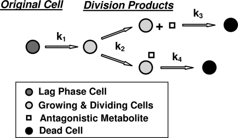
A unique approach to modeling bacterial growth and/or inactivation has been described by Taub et al., Doona et al., and Ross et al. (12, 28, 29). Their publications also provide an extensive literature survey of previous works on the subject. These researchers, affiliated with the U.S. Army Natick Soldier Research, Development and Engineering Center, produced a dynamics model of growth and death, which they termed a quasichemical model. Their basic assumption is that the increase (or decrease) in a microbial population is regulated by several rates: the physical growth rates of the individual cells prior to division, the rate of division once cells reach the appropriate size, and the rate of cell death via different mechanistic pathways, as shown schematically in Fig. 1. Since each rate has it own characteristic temperature dependence, the model allows for scenarios in which inactivation commences before there is any measurable growth. In other words, heat inactivation is just a special case in which the rate of cell death dominates over the rates of the other processes and consequently determines the treatment's time scale. The quasichemical model captures the essence of the growth-mortality duality, which plays a decisive role in the fate of microbial populations exposed to favorable, unfavorable, or lethal conditions. The above-described approach is not limited to temperature. The promoting or inhibitory factor can be the pH, the sugar concentration, high hydrostatic pressure, the presence of a chemical antimicrobial, or oxygen tension, etc. With its parameters adjusted, the quasichemical model can also be used to quantify the relative influences of the biological processes that control a population's growth or inactivation and how the population is affected by external conditions (12, 28, 29).

FIG. 1.

Cellular events from which the quasichemical model of microbial growth and mortality has been derived. Data are from Doona et al. (12).

Because the mechanisms that operate at the cellular level are rarely if ever known in sufficient detail, description of their dynamics may require a probabilistic approach. In contrast with traditional kinetic models, a probabilistic population model develops from the starting point that crucial information about the underlying processes is or may be missing. This is because the molecular events within the cells that determine the history of a microbial population, including its interaction with the habitat, are or can be too numerous and/or complex to be monitored and accounted for individually. The objectives of the present work are to explore the merits of the probabilistic approach to modeling microbial populations based on cell division and mortality, to develop a prototype of a general microbial growth and inactivation model, and to assess its potential applications.

METHODS

Simplified stochastic model of growth and mortality.

Consider a population of bacterial cells suspended in a medium of finite volume under conditions that favor growth, at least for some time. For the sake of simplicity, we will assume that an individual cell can be either viable or dead, deliberately ignoring the possibility that it can be injured and then recover or die at a later time. Microbial injury has been amply discussed in the literature (7, 8, 14). Its quantitative implications for food preservation processes have been recently addressed elsewhere (10) and will not concern us here. Similarly, when dealing with mortality, we will ignore the possibility of adaptation at sublethal temperatures or in the presence of a low chemical agent concentration, for example.

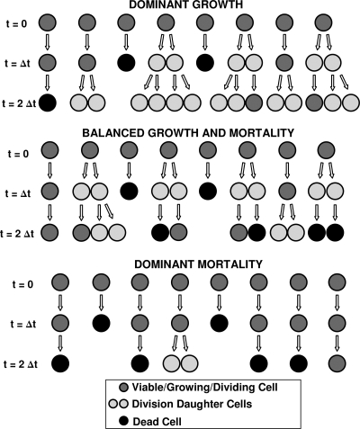
In principle, one can continuously monitor each cell, determine its size, assess its physiological state, and establish whether it is about to divide or die. Studies of this kind have actually been performed (1-4, 27), but there is little doubt that monitoring individual cells on a routine basis is impractical. The same can be said about counting the growing and dividing cells over short time intervals, on the order of minutes. Although a video camera and image-processing techniques can be used for the purpose, this approach would also be judged unfeasible under most circumstances. Without knowing the states of individual cells, all we can say is that, within a given time interval, every living cell has a certain probability that it will divide, a probability that it will expire, and a probability that it will remain alive but undivided, as shown in Fig. 2. Of course, these three probabilities must add up to 1, and in general they will be time dependent, as will be explained below. The development of a group of cells is shown schematically in Fig. 3. We will give a rigorous model for this situation in the next section, but for now we describe a simplified model that can be grasped more intuitively. We make the following two assumptions for this model. These can be checked by statistical techniques and are implicit in all the usual deterministic kinetic models.

FIG. 2.

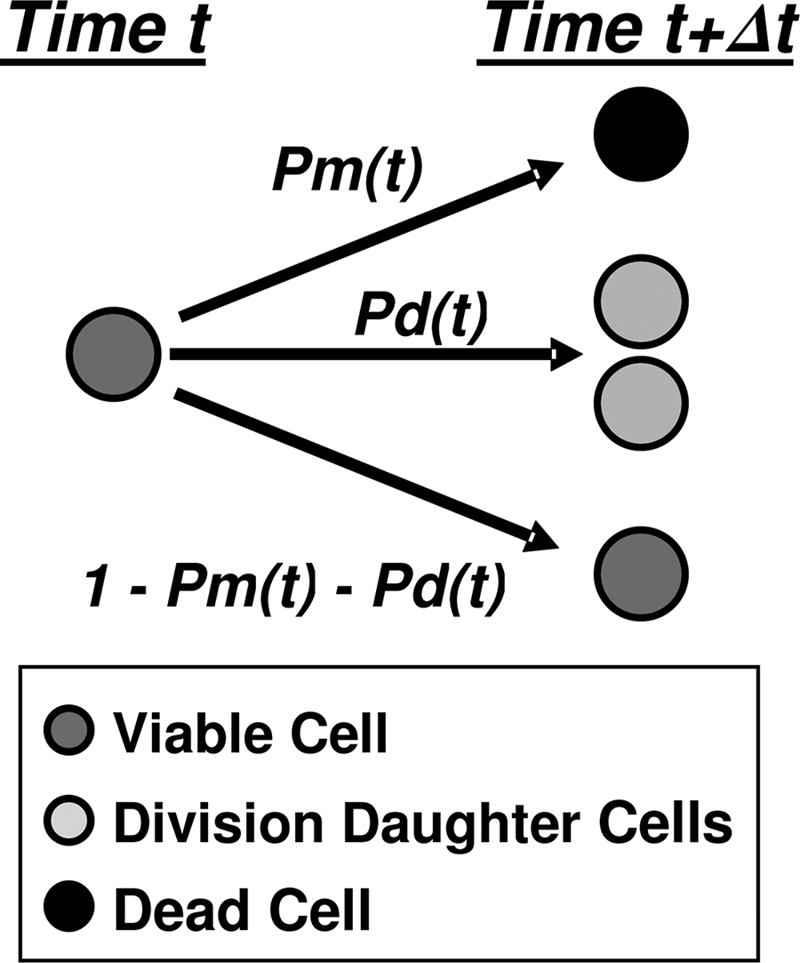
Cellular events from which the probabilistic model of microbial growth and mortality has been derived.

FIG. 3.

Microbial population dynamics at the cellular level.

(i) The fate of an individual cell can be treated mathematically as if it were independent of those of other cells.

(ii) The behavior of a cell alive at time t can be described mathematically as if it were independent of the past behavior of the whole population.

In other words, any actual interaction, current or previous, will be manifested in the division and mortality probability functions P_d(t) and P_m(t) but not in the structure of the model itself, again a testable hypothesis at least in principle. The same can be said about chemical changes in the habitat that growth may induce, like a drop in the pH or depletion of the dissolved oxygen. These possibilities too will be manifested in the probability functions P_d(t) and P_m(t) but not in the model's framework.

Consider a sequence of time points, 0 ≤ t₀ < t₁ < t₂ < …, which for simplicity we assume to be equally spaced, so that (t_{i + 1} − t_i) equals Δt for all values of i ≥ 0. For each individual cell alive at time t_i, the probability of dividing during the next Δt units of time is P_d(t_i)Δt, where P_d(t) is a specified function of time which gives the probability of division for an individual cell per unit of time (we refer to this as a transition rate function). Similarly, the probability of dying during the next Δt units of time is P_m(t_i)Δt, where P_m(t) is the specified transition rate for individual cell death. Finally, the probability of the cell's remaining alive but undivided is expressed as follows: 1 − [P_d(t_i) + P_m(t_i)]Δt. We observe that the transition rates P_d(t) and P_m(t) need not themselves be probabilities, i.e., they need not be less than 1 (they are ≥0, however). They become probabilities when multiplied by Δt. Notice that the probabilities of division and of death are proportional to Δt, consistent with the idea that these actions are less and less likely to occur over very short time intervals, i.e., as Δt approaches 0. Moreover, in view of assumption i, the probability that two or more cells will commence division or death during the same time interval will be proportional to (Δt)² and hence will become negligible for very short intervals. Notice that the transition rate P_d(t) is the limit, as Δt approaches 0, of the ratio Pr[cell divides during the time interval from t to (t + Δt)]/Δt, where Pr stands for probability. Consequently, P_d(t) may be construed as the instantaneous transition rate at time t. Similarly, P_m(t) is construed as the instantaneous transition rate for individual cell death at time t.

There is plenty of evidence that cells introduced into a new habitat, even a resource-rich habitat, may undergo a period of adjustment before they start to divide, hence the lag phase. Inevitably, substantial cell growth and division will deplete the nutrients and other resources in the habitat and will alter its chemical composition through the release of metabolites. Consequently, the individual transition rates P_d(t) and P_m(t) will not remain constant during the entire evolution of the population. Under most circumstances, one would expect the mortality transition rate, P_m(t), to be very low at the beginning, when the population density is low and resources are plentiful, and to increase when the population ages, resources are in short supply, the habitat becomes polluted, and there is fierce competition for space and nutrients. The cell division transition rate, P_d(t), may also be relatively low initially but will rise as the adjustment period comes to an end. However, as the cell density increases, conditions become less favorable for division. Consequently, the increase of P_d(t) will cease and the rate will eventually stabilize or decline. (Since at this stage mortality can take over, the whole division issue may become moot [see below].) Thus, both transition rates P_d(t) and P_m(t) must be functions of the population density and hence of time. In terms of the model, the continuously changing relation between these two functions will determine the observed growth/inactivation pattern of the population in question.

Let N(0) = N₀ be a given initial cell count, and let N(t_i) denote the population count (the number of live cells) at time t = t_i. These counts constitute a sequence of random variables that develop as follows: given that N(t_i) = n, the next count, N(t_{i + 1}), will be equal to (n + D_i − M_i), where D_i is the number of current cells that divide and M_i is the number that die. If we let L_i denote the number of cells that neither divide nor die, then L_i equals [n − (D_i + M_i)], and the joint distribution of the random variables (D_i, M_i, L_i) will be multinomial with corresponding probabilities {P_d(t_i)Δt, P_m(t_i)Δt, 1 − [P_d(t_i) + P_m(t_i)]Δt}. This, together with assumptions i and ii listed above, completely determines the probability structure of the stochastic process N(t_i), where i = 0, 1, 2, …. In particular, standard probability calculations show that, if N(t_i) = n, the probability of exactly one division and no deaths among the n cells currently alive is as follows: nP_d(t_i)Δt{1 − [P_d(t_i) + P_m(t_i)]Δt}^{n − 1} ∼ nP_d(t_i)Δt as Δt → 0. The probability of exactly one death and no divisions is obtained by interchanging the roles of d and m in these expressions. For the current population n, the limit, as Δt approaches 0, of the ratio Pr[exactly one cell divides during the time interval from t to (t + Δt)]/Δt is nP_d(t), which is the instantaneous transition rate for a cell division in the population. And similarly, the instantaneous transition rate for a death in the population is nP_m(t).

From this model, it is easy to calculate the expected population size at each time t_i. Given that N(t_i) = n and N(t_{i + 1}) = (n + D_i − M_i), the (conditional) expected value of N(t_{i + 1}) will be n{1 + [P_d(t_i) − P_m(t_i)]Δt}, and thus E[N(t_{i + 1})] equals E[N(t_i)]{1 + [P_d(t_i) − P_m(t_i)]Δt}, where E[…] indicates the expected value. A simple argument now shows that

(4)

where k is the number of steps.

Let us examine two extreme cases of the model, namely, those in which there are (essentially) (i) no deaths and (ii) no divisions. If during a given experimental period, P_d(t) ≫ P_m(t), then one should expect an exponential growth curve with the slope depending on the magnitude of P_d(t). In this case, the model gives

(5)

Likewise, if P_m(t) ≫ P_d(t), the result will be an inactivation curve

(6)

It can be shown analytically that, when Δt approaches 0, the expected value of the population size becomes, in the limit,

(7)

where s is a dummy variable.

In the two extreme cases described above, this gives exponential growth and decay, respectively, and the slope varies with time. The expected population size can itself provide a continuous, deterministic model. We discuss this in more detail below.

Stochastic process model of growth and mortality.

The models specified in equations 4 to 7 are fully deterministic. Given the values of the parameters, they allow for no uncertainty in the development of the microbial population, and they describe the population evolution as a smooth curve. Such a description may be appropriate for a large population of small units, such as microbes, and it may be possible in that situation to fit data with a continuous model. Such a description, however, will generally be unrealistic for small populations of cells. First of all, the number N(t) of live cells will not be a smooth function of time but rather a step function that changes values at the time of a cell division [N(t) → N(t) + 1] or death [N(t) → N(t) − 1], and as noted above, the probability of more than one division or death in a very short time interval will be negligible. Figure 3 illustrates that certain cells' lineages can proliferate while those of others remain stationary or die out. Also, a lineage that is relatively prolific at the beginning can become extinct for some reason while one that initially struggles may become invigorated after a few inactive generations. One can think of many other possible scenarios in which the trend for certain progeny changes or even reverses direction. Thus, regardless of the details, the emergence of a smooth growth curve for a very small microbial population is very unlikely. The same can be said about the inactivation of a small number of cells. Differences in resistance and/or ability to adapt or recover from injury among individual cells may be expressed in their deaths at irregular times. To account for the actual pattern of growth and mortality in small populations, let us monitor the fates of individual cells. Although the transition rates of division and mortality are fixed smooth functions, the fates of individual cells can vary dramatically. As illustrated in Fig. 3, a live cell at time zero can be found dead, still alive (but not divided), or already divided at time Δt.

The full stochastic model starts from the same assumptions, i and ii, given above but is developed in continuous time from the outset. To emphasize this, we write δt rather than Δt in what follows. By analogy to the simplified model, an individual cell alive at time t may divide with a probability of approximately P_d(t)δt during the time interval from t to t + δt, die with a probability of approximately P_m(t)δt, or remain alive but undivided with a probability of approximately 1 − [P_d(t) + P_m(t)]δt. (The reason for saying “approximately” is that, unlike the corresponding value in the simplified model, δt can vary. In fact, we will consider the limit as δt approaches 0. The final model will, of course, contain no such approximations.) The individual cell transition rates P_d(t) and P_m(t) have the same meaning as before: the (instantaneous) probabilities of division and mortality, respectively, per unit of time. As in the simplified model, the probability of two transitions (i.e., divisions or deaths) during very short time intervals is negligible. Let N(0) = N₀ be the initial population size, meaning the number of live cells, and let N(t) be the population size at time t of >0. The possible transitions of the stochastic process N(t) can be described as follows. Given that the population size at time t is N(t) = n, at time t + δt the population size can be N(t + δt) = n + 1, corresponding to a single cell division, N(t + δt) = n − 1, corresponding to a single death, or N(t + δt) = n, corresponding to no divisions or deaths, with (approximate) probabilities nP_d(t)δt, nP_m(t)δt, and 1 − n[P_d(t) + P_m(t)]δt, respectively; other values of N(t + δt) are possible, but with negligible probabilities. Of course, if the population becomes extinct at a certain time t, i.e., N(t) = 0, then no further divisions or deaths are allowed in the model.

The stochastic model is now characterized by saying that N(t) is a continuous-time, nonhomogeneous Markov chain, taking values in the nonnegative integers, with allowable transitions n → (n + 1) and n → (n − 1) (except that no transitions away from n = 0 are allowed). Such a Markov chain, whose only possible transitions are jumps with sizes of ±1, is called a birth and death process, and so we shall refer to this as the birth and death (BD) model. In this context, of course, birth corresponds to cell division. To complete the model, it suffices to specify the rates for each possible transition, and these are given by analogy to the simplified model, i.e., the transition rate at time t for the transition n → (n + 1) is nP_d(t), and for n → (n − 1), the rate is nP_m(t). In the case of the transition n → (n + 1), this means that the ratio P(N(t + δt) = n + 1|N(t) = n)/δt converges toward nP_d(t) as δt approaches 0. The intuitive meaning of this statement is that P(N(t + δt) = n + 1|N(t) = n) is ≈nP_d(t)δt when δt is very small, as indicated above, but notice that the limit of the ratio is exact. No approximation is involved. The discussion for the transition n → (n − 1) is similar, but with d replaced by m. (Nonhomogeneity refers to the time dependence of the transition rates.) The full mathematical development of Markov chains in general and of birth and death processes in particular is rather involved; Parzen (21) gives an accessible account of how this can be done.

According to our model, N(t) starts at N₀ when t = 0, remains there for a random period of time, and then makes a transition either to N₀ + 1 or N₀ − 1, corresponding to a cell division or a death. At later times, N(t) stays at its current value n for a random period of time and then makes the transition n → (n + 1) or n → (n − 1) (the latter cannot occur if n = 0) and continues on in the same fashion. No other transitions are possible.

The complete probabilistic description of a Markov chain typically involves solving an infinite system of differential equations (the Kolmogorov equations) for the transition probabilities of the chain. It is usually not feasible to solve these equations explicitly even in the special case of birth and death processes. Nonetheless, it is possible to obtain useful information about N(t) directly from the division and death rates. For example, the expected population size at time t and the probability that a microbial population will become extinct by time t are important quantities to know in the context of food safety; these can be determined explicitly (21). Let

(8)

where g(t) is the probability function limit.

The expected population size at time t in the BD model is the same as the expected population size as Δt approaches 0 in the simplified model, as follows:

(9)

The probability of extinction at time t, given an initial population of size N₀, is

(10)

The integral in this formula is generally difficult to evaluate in closed form but can be calculated numerically. Note that the probability of eventual extinction is obtained by letting t approach ∞ in the formula; in particular, Pr(population eventually extinct) equals 1 if and only if the integral (with upper limit t = ∞) is infinite. Observe also that the probability of extinction will be >0 except for a pure birth process, in which case P_m(t) is identically zero.

In addition, using a standard result in probability theory (Markov's inequality), we can at least give a bound on the probability that the population size exceeds a given threshold at time t. Let M be a given threshold; then Markov's inequality yields

(11)

Whether this bound is useful or not depends on the relative sizes of N₀ and M and on the particulars of the rate functions P_d(t) and P_m(t).

Continuous, large-population-limit model.

The discrete equation 4 can be converted into a continuous function by making the time intervals infinitesimally small, i.e., Δt → 0, and the number of steps infinitely large in the simplified model. In this case, the expected population size is given by the formula

(12)

where P_d(u) and P_m(u) are the individual cell division and mortality transition rates. As we have seen, this expression also represents the expected population size in the BD model. It is also possible to show that, if the population size is very large and the jumps of N(t) (with sizes of ±1) are scaled by the inverse of the population size, then the BD model will approach a deterministic, continuous curve, namely, f(t) = E[N(t)]. This is a form of the strong law of large numbers from probability theory and is related to so-called fluid limit models in queuing theory. Moreover, a form of the central limit theorem yields the conclusion that the error in approximating the BD model with the continuous large-population model will be a Gaussian stochastic process; this will be important for parameter estimation. Thus, the continuous curve f(t) may be justified as yet another continuous model for a large microbial population but one that is based on a simple, biologically motivated picture rather than the assumption of any particular type of kinetics. We refer to f(t) as the large-population (LP) model.

The integral in equation 12 can be integrated symbolically or numerically with a program like Mathematica (Wolfram Research, Champaign, IL), the program used in this work. For convenience, we will examine only the case in which the transition rates P_d(t) and P_m(t) are both logistic expressions that can be integrated in closed form. This facilitates the mathematical treatment of the model and shortens the calculation time considerably, especially when it comes to estimating the parameters of the model from simulated or actual growth/inactivation data (see below). The transition rates are as follows:

(13)

(14)

Consequently, the general version of the model has six parameters, p_d, k_d, t_d, p_m, k_m, and t_m. The function g(t) (the integral in equation 11) can be written explicitly in this case:

(15)

and then the function f(t) = N₀ exp[g(t)] becomes

(16)

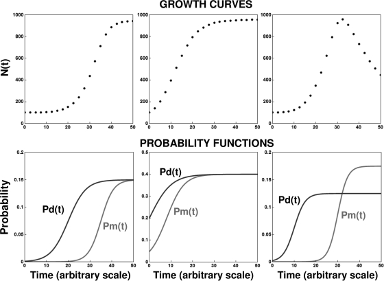
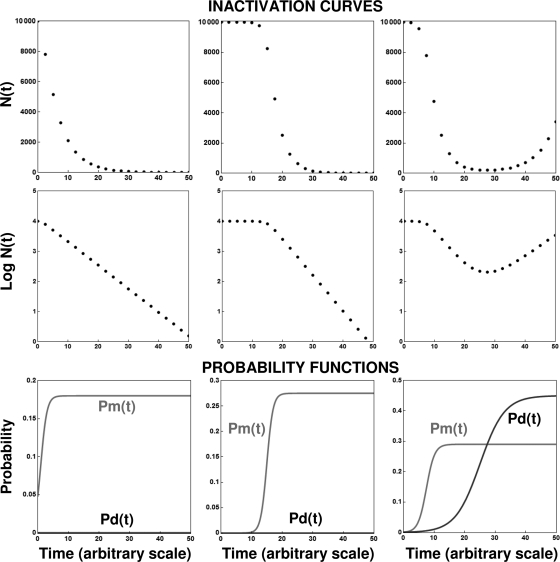
Notice that the model's six parameters can be reduced to five or even four for special cases. Examples are cases in which P_d equals P_m, as when the population size is stable for a sufficiently long time, and/or in which k_d can be assumed to equal k_m as a first approximation. The flexibility of the LP model is demonstrated in Fig. 4 and 5. Collectively, the two figures show very distinct population histories, from exponential or sigmoid growth, with and without a lag phase, to full inactivation, with and without a “shoulder,” as well as a continuous transition between growth and inactivation or vice versa. Yet all of the population histories were generated with a single general population model (equation 12) based on two underlying transition rate functions of the same kind (equations 13 and 14). As can be seen in these two figures, the different patterns were due to the temporal changes in the division and mortality rates, which in turn were controlled by the six parameters of the underlying probability rate functions. Similar growth and inactivation patterns can be generated with P_d(t) and P_m(t) defined by other expressions. The advantage of the logistic functions, apart from their mathematical convenience and the intuitive meaning of their parameters, is that when a growth curve has a plateau as in the stationary phase, then P_d(t) and P_m(t) in this region have the same value by definition. This greatly facilitates the model's construction by reducing the number of parameters and simplifying the estimation of its parameters from simulated or experimental data (see below). (For the total population size to remain unchanged, the number of cells added by division must be balanced by the number of dying cells or, which is less likely, not a single cell divides and none dies.)

FIG. 4.

Simulated isothermal microbial growth curves generated with the same deterministic continuous model (equation 14) and their corresponding division and mortality probability functions, P_d(t) and P_m(t), respectively. (Left) Growth curve with noticeable lag; (middle) growth without lag; (right) noticeable lag followed by a growth peak and intensive mortality. Notice that these very distinct growth patterns are all a manifestation of different relationships between underlying probability functions.

FIG. 5.

Simulated isothermal microbial survival (inactivation) curves generated with the deterministic continuous model (equation 14) plotted on linear and semilogarithmic coordinates. Also shown are the corresponding division and mortality probability functions, P_d(t) and P_m(t), respectively. (Left) Log-linear survival curve; (middle) curve with a flat shoulder; (right) inactivation followed by resumed growth. Notice that the different patterns were all produced with the same model (equation 14), which produced the growth curves shown in Fig. 4.

Nonisothermal growth and inactivation patterns.

The temperature effects on the fate of a microbial population are well known. Refrigeration in most cases slows down the growth or even decimates the cells. Elevating the temperature will have the opposite effect until it is raised to well above that optimal for growth, when it will cause mortality. Extreme cold can have a similar effect, albeit usually not at the same intensity and rate. In the lethal high-temperature regime, raising the temperature accelerates the inactivation dramatically. But there may be situations where premature cooling may allow the survivors to resume growth. A similar situation can also be observed in the case of disinfection with a volatile chemical agent, for example, where the treatment's survivors resume growth. The opposite may also occur. Raw foods are sometimes kept at a temperature that allows for microbial growth, but the population so created is destroyed by adequate cooking. Such growth/inactivation and inactivation/growth scenarios entail influences of temperature on the division and mortality rates and the manner in which these rates change with time. In the model outlined above, this implies that the coefficients of P_d(t) and P_m(t), defined by equations 13 and 14, are temperature dependent. Thus, when the temperature (T) varies with time [T = T(t)], the parameters p_d, p_m, k_m, k_d, t_d, and t_m will become functions of time and should be written as p_d[T(t)] and k_d[T(t)], etc., and equation 12 will then become a model of nonisothermal growth and inactivation. For almost all realistic nonisothermal temperature histories or profiles, especially when both heating and cooling are involved, the integral in equation 12 cannot be solved analytically. However, the integral can be solved numerically to produce the corresponding growth/inactivation curve. This applies to scenarios in which the temperature's rise or fall causes a transition from growth to inactivation or vice versa. The resulting patterns are similar in appearance to those shown in Fig. 4 and 5. The same can be said about scenarios involving oscillating temperatures. And as already stated, the growth-promoting or lethal agent need not be only temperature for the model to work. It can just as well be the oxygen tension, pH level, or hydrostatic pressure, etc., and combinations of these conditions. In such a case, P_d(t) will become P_d[T(t), pH(t)] instead of P_d[T(t)], say, and likewise for the other model parameters.

Simulations.

We give two simulation algorithms, one for tracking the development of individual cells and another for simulation at the population level, described in terms of the simplified model, of which the BD model is a continuous-time limit. We assume that the time interval over which the simulation is to take place is from t = 0 to t = t_f, 0 < t_f < ∞.

(i) Individual level.

(a) Choose the initial number, N₀, of live cells at time zero and the “time horizon,” t_f.

(b) Choose Δt small enough so that [P_m(t)+P_d(t)]Δt < 1 for 0 ≤ t ≤ t_f. [This is always possible as long as P_m(t) and P_d(t) are continuous functions of t.]

(c) At any time t = t_i = iΔt for which N(t) has been determined, draw a random number, R_n, with a uniform distribution between 0 and 1 (0 ≤ R_n ≤1), separately for each of the N(t) cells currently alive.

(d) For a particular cell, if R_n ≤ P_m(t)Δt, the cell dies; it will not be counted and will have no progeny. If P_m(t)Δt < R_n ≤ [P_m(t) + P_d(t)]Δt, the cell divides and now counts as two. If R_n > [P_m(t) + P_d(t)]Δt, the cell remains alive but undivided.

(e) Let N(t_{i + 1}) be the new number of living cells.

(f) Repeat steps c to e with i + 1 instead of i until the desired number of steps is reached.

Notice that since a new random number is drawn for each live cell and at each step, the growth/mortality curves generated with this algorithm will be irreproducible, unless the random number generator “seed” is fixed. After even a small number of iterations, the number of live cells can be very large, so the calculation can become overly burdensome very quickly. This imposes a practical limit on the number of initial cells that can be monitored and the number of steps in the growth/mortality curve construction. The following algorithm avoids this problem to an extent but can have numerical problems when the population size is large.

(ii) Population level.

(a′) Choose the initial number, N₀, of live cells at time zero and at the time horizon, t_f.

(b′) Choose Δt so that [P_m(t) + P_d(t)]Δt < 1 for 0 ≤ t ≤ t_f.

(c′) At any time t = t_i = iΔt for which N(t) = n has been determined, draw a (single) random number, R_n, with a uniform distribution between 0 and 1 (0 ≤ R_n ≤ 1).

(d′) If R_n ≤ nP_m(t)Δt{1 − [P_d(t_i) + P_m(t)]Δt}(n − 1), let N(t_i + 1) = n − 1; if nP_m(t)Δt{1 − [P_d(t_i) + P_m(t)]Δt}(n − 1) < R_n ≤ nP_m(t)Δt{1 − [P_d(t_i) + P_m(t)]Δt}(n − 1) + nP_d(t)Δt{1 − [P_d(t_i) + P_m(t)]Δt}(n − 1), let N(t_i + 1) = n + 1, and if R_n > nP_m(t)Δt{1 − [P_d(t_i) + P_m(t)]Δt}(n − 1) + nP_d(t)Δt{1 − [P_d(t_i) + P_m(t)]Δt}(n − 1), let N(t_i + 1) = n.

(e′) Repeat steps c′ to d′ with i + 1 instead of i until the desired number of steps is reached.

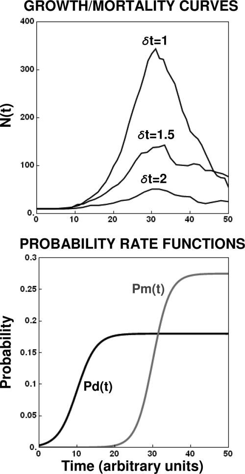
The effect of the choice δt on the curves produced by the individual-level algorithm is illustrated in Fig. 6. As δt becomes smaller, the generated growth curve becomes smoother and gets progressively closer to the continuous curve produced by the LP model based on the same underlying transition rates. As noted above, for computational reasons, the numbers generated by the stochastic (simplified) version of the model were too small to approach the LP-limit model. In some cases, the continuous LP model may not be a good approximation of the simulated model because a significant fraction of the cells can occasionally avoid mortality and exhibit extensive proliferation, resulting in a population size that will surpass that predicted by the LP model. Also, as shown above, except in the case of a “pure birth” process, there is a nonzero probability that the population becomes extinct, resulting in a growth curve that does not resemble the one predicted by the deterministic LP model.

FIG. 6.

Simulated growth curves generated with the discrete (stochastic) version of the model with the same underlying division and mortality probability functions but different δt's. Notice the curves' increased smoothness as δt decreases and N(t) increases.

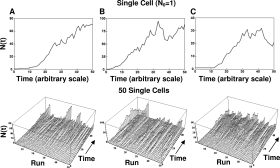
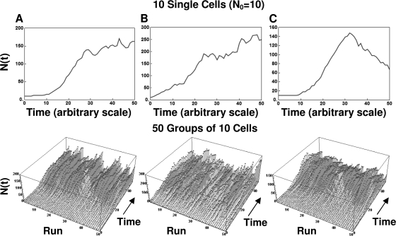
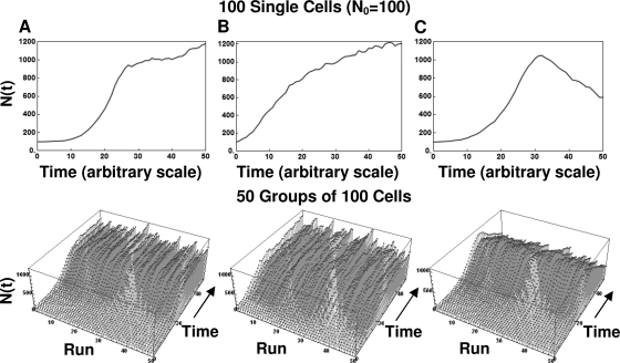
Examples of life histories of individual cells and their assemblies produced with the algorithm are shown in Fig. 7, 8, and 9. The figures show, from left to right, model-generated growth curves of three types: those with a noticeable lag, those with no lag, and those with a lag and peak growth followed by mortality. The top graphs are the growth curves, and the ones at the bottom are three-dimensional displays of the life histories of the individual cells (Fig. 7) or groups of 10 and 100 cells (Fig. 8 and 9, respectively). As in Fig. 4, the different growth patterns were created by adjusting the underlying transition rates. Figures 7 to 9 demonstrate that when the initial number of cells is very small, the fluctuations in the population size during its initial growth stage can be substantial. But if the population is initially large (or has reached a large size through successive divisions [Fig. 6]), its growth curve becomes progressively smoother. This result should not come as a surprise. When many cells divide or die according to the same rule, the averaging effect suppresses the fluctuations, which could be detected had the fate of each individual cell been monitored. This is the same effect that gives a smooth appearance to the growth curves of large populations of the kind reported in the literature and is a manifestation of the large population limit alluded to earlier.

FIG. 7.

Simulated growth curves started from a single cell generated with the discrete (stochastic) version of the model (equation 4), with different underlying division and mortality probability functions (top), and life histories of 50 such cells (bottom). (A) Growth with lag; (B) growth with no lag; (C) peaked growth with lag. Notice the jagged appearance of the curves.

FIG. 8.

Simulated growth curves started from a single group of 10 cells generated with the discrete (stochastic) version of the model (equation 4), with different underlying division and mortality probability functions (top), and life histories of 50 such groups of 10 (bottom). (A) Growth with lag; (B) growth with no lag; (C) peaked growth with lag. Notice that all the growth curves appear less jagged than those for the individual cells shown in Fig. 7.

FIG. 9.

Simulated growth curves started from a single group of 100 cells generated with the discrete (stochastic) version of the model (equation 4), with different underlying division and mortality probability functions (top), and life histories of 50 such groups of 100 (bottom). (A) Growth with lag; (B) growth with no lag; (C) peaked growth with lag. Notice that all the growth curves are smooth in comparison with those for the individual cells and smaller groups shown in Fig. 7 and 8, respectively.

The stochastic BD model provides a single conceptual framework for comparing the distinct growth and inactivation patterns of small and large microbial populations. It is an excellent tool for simulations, especially for a small initial number of cells and a limited number of generations. For larger population sizes, the LP model provides a biologically motivated, continuous, deterministic model.

Estimating the growth and mortality parameters from data.

If the functions P_d(t) and P_m(t) are known, except for the parameters p_d, k_d, and t_d, etc., then the parameters can be estimated from experimental (or simulated) isothermal growth and/or inactivation data by nonlinear regression or other methods of inference.

To demonstrate how the model parameters can be estimated from growth or inactivation data, we assume that the isothermal growth/inactivation of a hypothetical organism follows the LP model, equation 12, with transition (probability) rates P_d(t) and P_m(t) given by equations 13 and 14. To implement these assumptions, we wrote a program in Mathematica that generates growth/inactivation data using these models. The program, which has been posted as freeware on the Internet (http://www-unix.oit.umass.edu/∼aew2000/probabilistic_growth_and _mortality_model/ProbGrowthMortModel.html), comes in three versions based on equation 12, having four to six adjustable growth/mortality parameters. The program's three versions allow the user to generate data with specified parameter values, with either smooth patterns or added Gaussian random noise; to mimic experimental scatter in the counts; or to paste in experimental data instead of simulated data. The growth/inactivation data are then fitted with equation 12 by using Mathematica's nonlinear regression program, Nonlinear Model Fit. The estimated regression parameters are recorded, together with their statistical analysis and confidence intervals, and subsequently used to plot the fitted curve superimposed onto the data. On a separate graph, the corresponding estimated division and mortality transition rates P_d(t) and P_m(t) are also plotted.

As pointed out earlier, the continuous LP model differs from the BD model by a Gaussian stochastic process. In general, this error process will be correlated, though it can be expected that the correlations will be short range and hence will die out for widely separated times. Thus, it is reasonable in simulations to use Gaussian random (i.e., uncorrelated) noise for the error process. In analyzing real data, correlated errors will mean that parameter estimates are less efficient (in the technical statistical sense), but this should have little effect in practice.

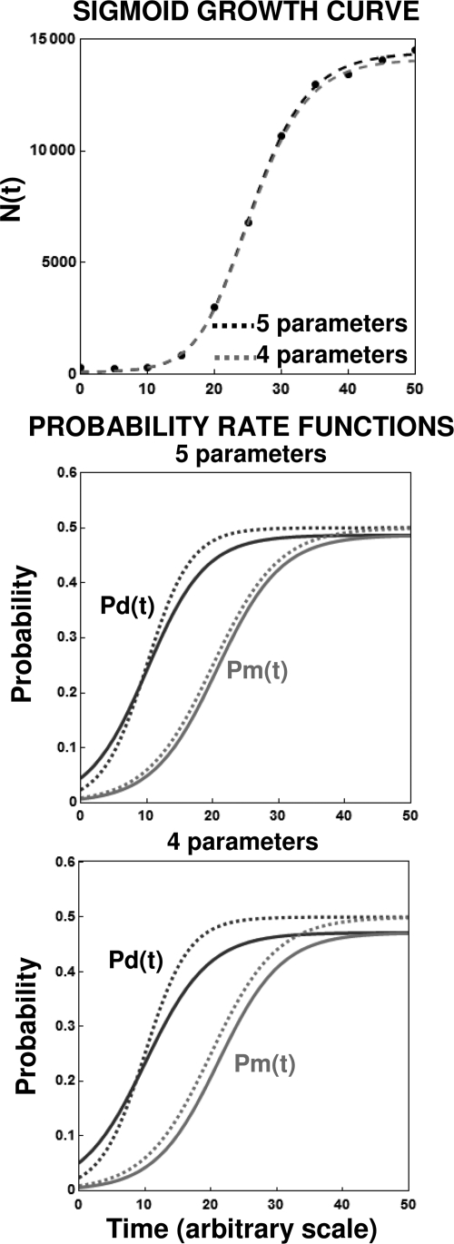
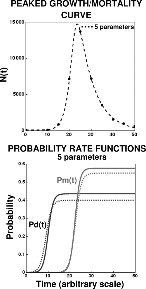
An example of a simulated realistic-looking sigmoid growth curve is shown in Fig. 10. The data were generated by the program with a small amount of random noise equivalent to 5% of the smooth N(t) level. Since at the plateau region (stationary phase) according to our model, P_d(t) = P_m(t) and p_d = p_m = p, we are left with four or five adjustable parameters depending on whether k_d and k_m are assumed to be equal or not. As can be seen in the figure (top plot), the data can be fitted with both the four- and five-parameter versions of the model. The two versions of the model yielded similar division and mortality transition rates, as shown in the middle and bottom plots, as well as similar growth/mortality parameters, as shown in Table 1; we could, of course, perform a formal statistical test to determine which of these two models is more appropriate. We note that agreement of the kind shown in Fig. 10 can be achieved only with a relatively large number of data points and/or small scatter. A more complicated example, with growth followed by mortality, is shown in Fig. 11. In this case, however, since P_m is >P_d, only a model with at least five parameters was required to retrieve the functions P_d(t) and P_m(t), which are also shown in the figures. Although the general features of the underlying mobility were recovered, as shown in the figure and Table 1, this was possible because of the relatively small scatter of the generated data.

FIG. 10.

Extraction of the division and mortality probability functions from simulated sigmoid growth data with small scatter. (Top) Fit of the four- and five-parameter versions of equation 16; (middle and bottom) corresponding probability functions calculated with the regression parameters (solid lines) and those used to create the data (dashed lines). Notice the similarity between the division and mortality probability functions estimated by the four- and five-parameter deterministic models (equations 15 and 16, respectively). The parameters for the shown data points’ generation and the retrieved parameters are listed in Table 1.

TABLE 1.

Parameters for growth data generation and retrieved parameters using equation 16 as a model with equations 13 and 14 as the probability rate functions

Parameter type	Sigmoid growth curvea					Peaked growth/mortality curveb
	Pd = Pm	kd	km	tcd	tcm	Pd	Pm	k	tcd	tcm
Parameters for data generation	0.5	0.3	0.2	10	20	0.4	0.55	0.75	9	22.5
Retrieved parameters
Parameters for four-parameter version	0.47	0.21	0.21	10.1	21.2
Parameters for five-parameter version	0.49	0.23	0.21	10.1	20.7	0.43	0.58	0.88	10.1	22.3

^aExamples are shown in Fig. 10.

^bExamples are shown in Fig. 11.

FIG. 11.

Extraction of the division and mortality probability functions from a simulated peaked growth curve. (Top) Fit of the five-parameter version of equation 16; (bottom) corresponding probability functions calculated with the regression parameters (solid lines) and those used to create the data (dashed lines). The parameters for the shown data points’ generation and the retrieved parameters are listed in Table 1.

RESULTS AND DISCUSSION

Analysis of published growth curves.

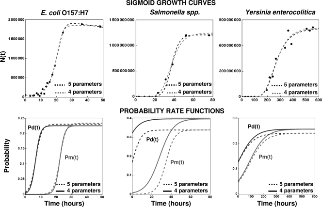
Published sigmoid growth data on Escherichia coli O157:H7, Salmonella spp., and Yersinia enterocolitica (18) (see ComBase record numbers B124_39 and B002_146 at http://combase.arserrc.gov/), together with the fit of equation 16 as the model, are shown in Fig. 12. Also shown in the figure are the corresponding probability rate functions P_d(t) and P_m(t) calculated with the four- and five-parameter versions of the model. In the cases of E. coli and Yersinia, the calculated values were almost identical. In the case of Salmonella spp., they had a considerable gap but showed the same general trend nevertheless.

FIG. 12.

Experimental sigmoid growth curves for E. coli O157:H7, Salmonella spp., and Y. enterocolitica fitted with the four- and five-parameter versions of equation 16 as a model (top) and the corresponding estimated underlying division and mortality probability functions (bottom). The experimental data are from Koseki and Isobe (18) and the Food Standard Agency (http://combase.arserrc.gov/; record numbers B124_39 and B002_146), respectively.

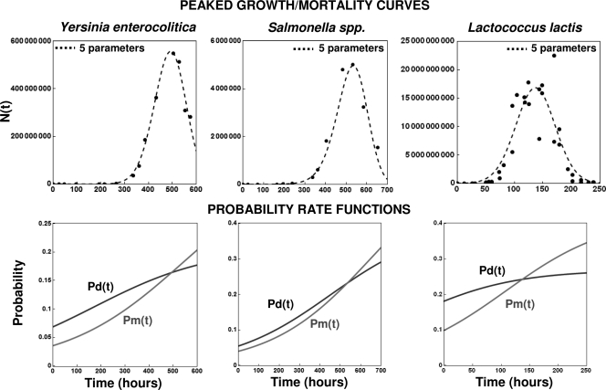
Figure 13 shows published growth/mortality data on Lactococcus lactis, Y. enterocolitica, and Salmonella spp. (13) (see ComBase record numbers B092_4 and B002_92 at http://combase.arserrc.gov/), together with the fit of equation 16 as a model. The corresponding transition rates P_d(t) and P_m(t), calculated with the five-parameter version of the model, are shown at the bottom of the figure. Because all the curves have a clear peak, the parameters p_d and p_m have different values, thus requiring the five-parameter model version for their calculation. The figure demonstrates again that it is possible to estimate the cell division and death transition rates from experimental growth/mortality data.

FIG. 13.

Experimental peaked growth/mortality curves for Y. enterocolitica, Salmonella spp., and L. lactis fitted with the five-parameter version of equation 16 as a model (top) and the corresponding estimated underlying division and mortality probability functions (bottom). The experimental data are from the Food Standard Agency (http://combase.arserrc.gov/; record numbers B092_4 and B002_92) and Dougherty et al. (13), respectively.

Admittedly, we have deliberately chosen data that are sufficiently dense and have a relatively small visible scatter. The method may not have yielded meaningful results had a data set with a smaller number of points and/or larger scatter been used. At this point, the functions P_d(t) and P_m(t) in the above-described example are hypothetical at best. It is, of course, possible to pursue formal statistical tests of these or other plausible models, but the purpose of the examples was to present a feasible methodology, not to investigate the particular organisms. Thus, we have illustrated parameter estimation using the LP model, which can be analyzed using standard nonlinear regression software, rather than the BD model. Statistical analysis of nonhomogeneous Markov chain data, as in the case of the BD model, by maximum likelihood, for example, would require explicit determination of the transition probability functions of the Markov chain, generally a daunting task. Other approaches, such as the method of moments, could also be used. But here again, our primary goal was to establish a unified view of microbial growth and mortality via stochastic modeling, rather than engage in statistical analysis of particular data sets.

Concluding remarks.

Most microbial kinetic models for foods have been developed in order to quantify and predict growth and inactivation patterns at the population level. Only a few modelers, notably Baranyi (2, 4), Brul et al. (6), Pin and Baranyi (27), and the Natick group (Taub et al. [29], Doona et al. [12], and Ross et al. [28]), have tried to link observed growth and inactivation kinetics to processes or events at the cellular level directly. The model described in this work is not intended to replace existing kinetic models of either kind. The main reason for its introduction is to provide a general complementary tool to interpret population evolution patterns of cell division and mortality. The approach has already been successfully implemented in the interpretation of pure inactivation patterns, such as those encountered in heat treatments at lethal temperatures. Since, with few exceptions, growth and division do not occur during such treatments, the survival curve is by definition a manifestation of the mortality events' temporal distribution, akin to (but not the same as) P_m(t) in the growth/mortality model. In that case, therefore, the distribution of the cells' death times can be estimated directly from the experimental survival data (24, 25). In contrast, the present work is concerned with the whole process of cell division, as well as mortality. Although the stochastic BD model may not be simple enough for everyday use, it does give a unified conceptual explanation of why different growth and inactivation patterns emerge. On the other hand, explicit formulas are also given for the expected population size, the probability of extinction, and a bound for the probability that the population size will exceed a given threshold, all in terms of the transition (probability) rates. These quantities, which can be estimated from original or published experimental data for large populations obtained by standard methods of the field, may be useful to the food, pharmaceutical, and fermentation industries as well as public health authorities. Stochastic modeling provides a tool with which to simulate microbial population processes and investigate their characteristics and eliminates the need to make kinetic assumptions that are usually hard and sometimes impossible to confirm.

The starting point of the probabilistic approach is the admission either that we do not know what happens at the cellular level or that our knowledge is insufficient to derive a plausible mechanistic model. Nevertheless, this work shows that it is possible to translate the probabilities of important events in the life cycle of individual cells into commonly observed growth and inactivation patterns and transitions between them. The work also shows that it is possible to estimate an organism's division and mortality transition rates from experimental data, at least if they are specified in parametric form. The quality of the estimates will depend on the complexity of the model and the amount and scatter of the data. Techniques to monitor the states of individual cells, through image processing, for example, already exist and may eventually be used to validate and improve the modeling approach. For now, experimental evidence can be used to test any specified structure of the transition rates P_d(t) and P_m(t), whether logistic or other, or to suggest alternative mathematical expressions to describe them.

Although much of the discussion in this article focuses on temperature as a promoter of growth or cause of inactivation, the general concept is just as applicable to other factors that make a habitat and conditions favorable or hostile to microbial growth or survival. Possible examples are chemical disinfectants and preservatives, biological antimicrobials, water activity, pH, oxygen tension, and CO₂ pressure, etc.

The stochastic BD model may be particularly useful to simulate and investigate the growth and mortality patterns of very small microbial populations, for which most if not all the traditional deterministic continuous models may not be suitable. Microbial infection or accidental contamination of a food need not always start with massive invasion by the pathogen or spoilage organism. The former, especially, can start with the ingestion of or contact with a small number of cells. According to the described model, this means that some groups of cells will die off while others may proliferate to various degrees. It also means that both the initial inoculum size and the vigor of the pathogen cells, expressed as P_d(t) vis-à-vis P_m(t) in terms of the model, will affect the fraction of exposed persons that will eventually become sick. In the case of a spoilage organism, both factors will determine the number of food units that will actually be spoiled and to what extent. As the simulations in Fig. 7 to 9 demonstrate, not all exposed persons or contaminated units will be equally affected, even if they have received the same dose. These are qualitative predictions that are consistent with observation. The concept described above also applies to scenarios in which the microbial population size progressively decreases rather than increases. But one has to distinguish between growth suppression caused by refrigeration or an antimicrobial at a low concentration, say, and massive rapid mortality as in the case of heat sterilization or pasteurization. In thermal preservation, the treatment is almost always much shorter than the cells' division time, resulting in a practically zero and irrelevant division probability rate, P_d(t). The stochastic version of the model can be useful in simulating the potential fates of a small number of individual cells or groups of cells, especially if they are present in a relatively protected locale, such as the surface of an air bubble. The probabilistic modeling approach can be extended to bacterial spores' germination. This, however, will require revision of the model to account for the probability of germination and, in the case of certain bacillus spores, that of activation as well.

REFERENCES

- 1.Balaban, N. Q., J. Merrin, R. Chait, L. Kowalik, and S. Leiber. 2004. Bacterial persistence as a phenotypic switch. Science 305:1622-1625. [DOI] [PubMed] [Google Scholar]
- 2.Baranyi, J. 2002. Stochastic modelling of bacterial lag phase. Int. J. Food Microbiol. 73:203-206. [DOI] [PubMed] [Google Scholar]
- 3.Baranyi, J., C. Pin, and T. Ross. 1999. Validating and comparing predictive models. Int. J. Food Microbiol. 48:159-166. [DOI] [PubMed] [Google Scholar]
- 4.Baranyi, J. 1998. Comparison of stochastic and deterministic concepts of bacterial lag. J. Theor. Biol. 192:403-408. [DOI] [PubMed] [Google Scholar]
- 5.Baranyi, J., and T. A. Roberts. 1994. A dynamic approach to predicting bacterial growth in food. Int. J. Food Microbiol. 23:277-294. [DOI] [PubMed] [Google Scholar]
- 6.Brul, S., F. I. C. Mensonides, K. J. Hellingwerf, and M. J. Teixeira de Mattos. 2008. Microbial systems biology: new frontiers open to predictive microbiology. Int. J. Food Microbiol. 128:16-21. [DOI] [PubMed] [Google Scholar]
- 7.Busta, F. F. 1976. Practical implications of injured microorganisms in food. J. Milk Food Technol. 39:138-145. [Google Scholar]
- 8.Cazemier, A. E, S. F. M. Wagenaars, and P. F. ter Steeg. 2001. Effect of sporulation and recovery medium on the heat resistance and amount of injury of spores from spoilage bacilli. J. Appl. Microbiol. 90:761-770. [DOI] [PubMed] [Google Scholar]
- 9.Corradini, M. G., and M. Peleg. 2007. The non-linear kinetics of microbial inactivation and growth, p. 129-160. In S. Brul, M. Zwietering, and S. van Gerwen (ed.), Modelling microorganisms in food. Woodhead Publishing, Cambridge, United Kingdom.
- 10.Corradini, M. G., and M. Peleg. 2007. A Weibullian model of microbial injury and mortality. Int. J. Food Microbiol. 119:319-328. [DOI] [PubMed] [Google Scholar]
- 11.Corradini, M. G., and M. Peleg. 2006. On modeling and simulating transitions between microbial growth and inactivation or vice versa. Int. J. Food Microbiol. 108:22-35. [DOI] [PubMed] [Google Scholar]
- 12.Doona, C. J., F. E. Feeherry, and E. W. Ross. 2005. A quasi-chemical model for the growth and death of microorganisms in foods by non-thermal and high-pressure processing. Int. J. Food Microbiol. 100:21-32. [DOI] [PubMed] [Google Scholar]
- 13.Dougherty, D. P., F. Breidt, R. F. McFeeters, and S. R. Lubkin. 2002. Energy-based dynamic model for variable temperature batch fermentation by Lactococcus lactis. Appl. Environ. Microbiol. 68:2468-2478. [DOI] [PMC free article] [PubMed] [Google Scholar]
- 14.Feeherry, F. E., D. T. Munsey, and D. B. Rowley. 1987. Thermal inactivation and injury of Bacillus stearothermophilus spores. Appl. Environ. Microbiol. 53:365-370. [DOI] [PMC free article] [PubMed] [Google Scholar]
- 15.Fujikawa, H., A. Kai, and S. Morozumi. 2004. A new logistic model for Escherichia coli growth at constant and dynamic temperatures. Food Microbiol. 21:501-509. [Google Scholar]
- 16.Holdsworth, D., and R. Simpson. 2007. Thermal processing of packaged foods. Springer, New York, NY.
- 17.Jay, J. M. 1996. Modern food microbiology. Chapman & Hall, New York, NY.
- 18.Koseki, S., and S. Isobe. 2005. Prediction of pathogen growth on iceberg lettuce under real temperature history during distribution from farm to table. Int. J. Food Microbiol. 104:239-248. [DOI] [PubMed] [Google Scholar]
- 19.McKellar, R., and X. Lu (ed.). 2004. Modeling microbial responses on foods. CRC Press, Boca Raton, FL.
- 20.McMeekin, T. A., J. N. Olley, T. Ross, and D. A. Ratkowsky. 1993. Predictive microbiology: theory and application. John Wiley & Sons, New York, NY.
- 21.Parzen, E. 1962. Stochastic processes. Holden-Day, San Francisco, CA.
- 22.Peleg, M., M. G. Corradini, and M. D. Normand. 2007. The logistic (Verhulst) model for sigmoid microbial growth curves revisited. Food Res. Int. 40:808-819. [Google Scholar]
- 23.Peleg, M. 2006. Advanced quantitative microbiology for food and biosystems: models for predicting growth and inactivation. CRC Press, Boca Raton, FL.
- 24.Peleg, M. 2003. Microbial survival curves: interpretation, mathematical modeling and utilization. Comments Theor. Biol. 8:357-387. [Google Scholar]
- 25.Peleg, M., and M. B. Cole. 1998. Reinterpretation of microbial survival curves. Crit. Rev. Food Sci. 38:353-380. [DOI] [PubMed] [Google Scholar]
- 26.Peleg, M. 1996. A model of microbial growth and decay in a closed habitat based on combined Fermi's and the logistic equations. J. Sci. Food Agric. 71:225-230. [Google Scholar]
- 27.Pin, C., and J. Baranyi. 2006. Kinetics of single cells: observation and modeling of a stochastic process. Appl. Environ. Microb. 72:2163-2169. [DOI] [PMC free article] [PubMed] [Google Scholar]
- 28.Ross, E. W., I. A. Taub, C. J. Doona, F. E. Feeherry, and K. Kustin. 2005. The mathematical properties of the quasi-chemical model for microorganism growth-death kinetics in foods. Int. J. Food Microbiol. 99:157-171. [DOI] [PubMed] [Google Scholar]
- 29.Taub, I. A., F. E. Feeherry, E. W. Ross, K. Kustin, and C. J. Doona. 2003. A quasi-chemical kinetics model for the growth and death of Staphylococcus aureus in intermediate moisture bread. J. Food Sci. 68:2530-2537. [Google Scholar]
- 30.van Impe, J. F., F. Poschet, A. H. Geeraerd, and K. M. Vereecken. 2005. Towards a novel class of predictive microbial growth models. Int. J. Food Microbiol. 100:97-105. [DOI] [PubMed] [Google Scholar]
- 31.Zwanzig, R. 1973. Generalized Verhulst laws for population growth. Proc. Natl. Acad. Sci. U. S. A. 70:3048-3051. [DOI] [PMC free article] [PubMed] [Google Scholar]