MMBGX: a method for estimating expression at the isoform level and detecting differential splicing using whole-transcript Affymetrix arrays

Abstract

Affymetrix has recently developed whole-transcript GeneChips—‘Gene’ and ‘Exon’ arrays—which interrogate exons along the length of each gene. Although each probe on these arrays is intended to hybridize perfectly to only one transcriptional target, many probes match multiple transcripts located in different parts of the genome or alternative isoforms of the same gene. Existing statistical methods for estimating expression do not take this into account and are thus prone to producing inflated estimates. We propose a method, Multi-Mapping Bayesian Gene eXpression (MMBGX), which disaggregates the signal at ‘multi-match’ probes. When applied to Gene arrays, MMBGX removes the upward bias of gene-level expression estimates. When applied to Exon arrays, it can further disaggregate the signal between alternative transcripts of the same gene, providing expression estimates of individual splice variants. We demonstrate the performance of MMBGX on simulated data and a tissue mixture data set. We then show that MMBGX can estimate the expression of alternative isoforms within one experimental condition, confirming our results by RT-PCR. Finally, we show that our method for detecting differential splicing has a lower error rate than standard exon-level approaches on a previously validated colon cancer data set.

INTRODUCTION

Oligonucleotide microarrays allow biomedical researchers to estimate the expression of thousands of genes simultaneously through their mRNA transcripts. Labelled fragments of the transcripts in the form of single-stranded RNA or DNA are hybridized onto an array containing hundreds of thousands of complementary DNA 25-mers and then scanned. The colour intensities at each probe reflect the degree of hybridization and form the raw data used to make inference on transcript abundance in the sample.

Traditional Affymetrix arrays, 3′ GeneChips, use perfect match (PM) and mismatch (MM) probe pairs that target the 3′-end of each gene of interest via its RNA products. The PM probes match the target transcript exactly, whereas the MM probes match it exactly but for a complementary base on the 13th position. The purpose of the MM probes is to capture the degree to which RNAs other than the target transcripts bind to the corresponding PM probes (i.e. non-specific hybridization). The probes on 3′-arrays have been found to exhibit varying propensities to bind to target RNA according to the base composition of their sequences (1) and methods for estimating expression levels that incorporate probe affinity effects have shown demonstrable advances over methods in which these effects are ignored (2,3).

In whole-transcript arrays, PM probes are distributed over the whole length of each gene and probe affinity effects can be estimated according to GC content, the proportion of G and C bases in the sequence. Rather than one MM probe for each PM probe, they contain several hundred ‘background probes’ for each of the 26 possible GC proportions on the PM probes (4). In contrast with existing methods, which use point estimates (5,6) or probe filtering [cf. DABG in (7)] to account for non-specific hybridization, we use the empirical distribution of the GC-specific background probe intensities to fully incorporate the background noise uncertainty into our modelling of the data (cf. Supplementary Figure S1).

Both 3′ and whole-transcript arrays contain probes that map to multiple transcribed locations on the genome and are therefore prone to hybridizing perfectly to transcripts other than the intended target (Figure 1A). On the human Gene 1.0 ST array, for instance, almost one in 10 gene-targeting probesets contain one or more probes mapping to non-target genes. If this effect is not accounted for, signal extraction algorithms may yield biased results. This bias is observed in real data where the PM intensities of probes that map to multiple targets are on average consistently higher than those of single-match probes (Supplementary Figure S2).

Figure 1.

Illustration of the two types of multi-match probes. (A) One probe shares a subsequence with two separate transcribed regions. Such a probe would belong to two probesets—one targeting each region. (B) Probes under the leftmost exon capture signal from isoform 1, while the other probes capture signal from isoforms 1 and 2. In order to estimate expression at the isoform level, probes should be grouped into two probesets—one targeting each isoform. If both isoforms are present in the sample, the probe signal will tend to be higher at the multi-match probes than at the single-match probes.

An additional kind of multi-mapping may be modelled in the denser Exon arrays: the mapping of probes to exons belonging to different isoforms of the same gene, an effect that may be exploited to detect alternative and differential splicing (Figure 1B). Current methods for Exon arrays (8,9) focus on detecting large changes in the expression of individual exons relative to the gene. Thus they do not detect nor quantify the abundance of each individual isoform. Our model can directly estimate isoform-level expression and therefore can be used to compare the expression of variants between conditions and even within one sample.

Bayesian hierarchical modelling provides a coherent framework for making inference from data with a nested structure. As such, it can be usefully applied to microarray data (3,10,11), where parameters may be shared at different levels, ranging from probes and probesets to array samples and biological or technical conditions. Here, we present a fully hierarchical Bayesian model for expression analysis, MMBGX, that takes into account the design of the new arrays and the one-to-many mappings between probes and probesets. We have constructed graphs of these mappings for two types of probesets. On the Gene arrays, we use probesets that represent genes as annotated by Affymetrix and on the Exon arrays, we use probesets that represent genes or transcripts (i.e. isoforms) as annotated by (12). We show evidence of the bias incurred if multi-mapping is not taken into account and demonstrate the ability of MMBGX to disaggregate the signal between various isoforms of the same gene. The method provides posterior summaries for each gene or transcript that encode the full uncertainty in the expression parameter estimates and may be used to detect differential expression (13). The implementation uses a recently developed adaptive Markov chain Monte Carlo (MCMC) algorithm (14) and shared-memory parallelism to achieve good computational performance. In the ‘Results’ section, we assess the method using simulated and real Gene array data, comparing our gene-level results with those of two other widely available methods. We then present the results of our transcript-level analysis on a single-condition mouse Exon array data set and validate some of our predictions by RT-PCR. Finally, we compare MMBGX's; ability to detect differential splicing between experimental conditions to a standard exon-level approach by analysing a previously published and validated colon cancer data set. Note that throughout the article, we use the phrase ‘differential splicing’ to refer to gene-normalized differential transcript expression, which may involve more than one splice site, as well as the usual meaning of gene-normalized differential inclusion of a single exon. The MMBGX software package and accompanying instructions are freely available from http://bgx.org.ukhttp://bgx.org.uk.

MATERIALS AND METHODS

Re-annotation of Exon array probes

The Exon arrays contain a large superset of the probes in the Gene arrays, covering virtually every known exon on the target genomes, and thus permitting expression summarization at the exon level. While exon and gene-level expression summarization may reveal useful differences in exon retention or exclusion patterns across samples, it is the quantification of alternative splice variants—the ultimate determinants of protein products—that is biologically most interesting.

In order to address this challenge, we required a re-annotation of the probes on the Exon arrays that group them into probesets that target transcripts rather than genes or exons. Our aim was to construct a graph between probes and probesets largely based on the phenomenon illustrated in Figure 1B. A solution was found by combining the Ensembl database, which contains tens of thousands of known transcripts, with X:Map (15), which contains hits between Affymetrix probes and Ensembl transcripts. In this way, probes are grouped into probesets that target any number of transcripts, be they alternative isoforms of the same gene or transcripts from entirely separate genes.

Hierarchical model

Using the BGX method (3,11) for the analysis of 3′ GeneChips as a starting point, we developed a new model that (i) accounts for the use of global GC content-specific background probes instead of probe-specific MM probes and (ii) accounts for the complex mapping between probesets and probes explicitly. Signal from multi-match probes is split in a logical way to obtain unbiased estimates of expression at the gene level for Gene arrays and the transcript or gene level for Exon arrays. While probes may be grouped into probesets that target genes as well as individual transcripts, for simplicity, we refer to probeset targets only as ‘transcripts’ below.

Perfect match probe intensities, PMs, are modelled as arising partly from specific hybridization, S (the signal), and partly from non-specific hybridization, H, both of which are probe (j), condition (c) and replicate (r) specific:

1

Note how, unlike Equation (4.1) in Hein et al. (11), Equation (1) does not group probes into probesets, thus accommodating for the fact that one or more transcripts may contribute to the signal intensity observed at a PM probe. Also, we do not assume an additional additive error, as the model would then be overparameterized. The quantity of interest is the unknown signal, S_jcr, and H_jcr encapsulates the noise.

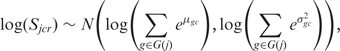
We wish to model the signal on the log-scale to account for multiplicative error. In the simple case where a single transcript g in condition c is linked to the probe signal, S_jcr, this suggests the model

2

where μ_gc is the probeset-level log expression measure, σ_gc² is an error term and in this case there is a one-to-one mapping from probe j to probeset g.

We know from the multi-mapping structure, however, that two or more transcripts may in fact contribute to the signal. We therefore need to model the contribution of each transcript to the signal of one probe. We assume that the contribution to the signal and its variance is additive on the real scale. This assumption is based on the fact that the means and variances of multi-match probes are consistently higher than those of single-match probes (Supplementary Figure S2). Since the μ_gc and σ_gc² parameters are on the log-scale but their contribution to the signal are additive on the real scale, we need to exponentiate before summing and finally go back to the log-scale. Allowing for any number of transcript contributions to the signal, the signal parameter, S_jcr, therefore follows the following distribution:

3

where G( j ) indexes the set of transcripts matched by probe j [see Figure 2 for graphical examples of G( j )]. When G( j ) contains only one index, Equation (3) reduces to the simpler Equation (2).

Figure 2.

A cluster of interconnected probesets on the human Gene 1.0 ST array. The ellipses represent probesets and the dots represent probes. Probesets are linked to their component probes by edges. For example, probeset 7926979, which probes a region on chromosome 10, and probeset 8132692, which probes a region on chromosome 7, share two probes. Probesets 7988175 and 7988206 are identical but nominally probe two separate regions on chromosome 15. As an example of Equation (3), if j indexed either of the two probes linking probesets 7927979 and 8132692, then the elements of G(j) would be the indices of probesets 7927979 and 8132692.

The non-specific binding parameter, H, log-transformed, follows a GC content (k)- and array (r)- specific normal distribution:

4

where k(j) indexes the GC content category of probe j.

The mean and variance, and , respectively, are estimated empirically from the logarithms of the GC content-specific background probes. While most methods plug the median background measurement into the non-specific hybridization parameter (in our case, H_jcr) (5,6), we allow a degree of variability, consistent with the observed variability in background probe measurements (Supplementary Figure S1). Thus, the model accounts for PMs that are lower than the corresponding median background measurement through allowing a lower H, rather than relying solely on a high error in the signal, which may bias this error upwards.

We conclude the full specification of our model by assuming priors similar to those used in BGX (11). We place a U(0,15) prior on μ_gc, which amply covers the range of possible expression values, a N(α_c,β_c²) prior on and a Γ(1.2,0.2) prior on . Note that a lower bound of 0 on μ's; prior restricts the mean of S to a minimim value of 1 even though theoretically it may be as low as 0. However, a comparison of the model with an alternative less-computationally tractable model in which follows a truncated normal distribution [as in (11)] showed that they gave virtually indistinguishable results. Specifying a prior for α_c leads to slow mixing of the MCMC sampler, making reliable inference computationally inefficient. We therefore developed an empirical Bayes algorithm that estimates α_c accurately and fix it to this value (see Algorithm S1 in the Supplementary Data). In the process, estimates of S_jcr, H_jcr, μ_gc, σ_gc² and β_c² are computed and set to starting values for the respective samplers in order to speed up convergence. The central parameter of Equation (3), μ_gc, acts as the transcript-level log expression measure.

Detecting differential splicing

Using the posterior distribution of log expression for genes and their transcript variants, we devised the following statistic as a measure of the probability of differential splicing:

5

where μ_tc is the expression level of transcript t in condition c and μ_g(t)j is the expression level of the gene containing transcript t in condition c. The quantity p_t is the posterior probability that transcript t is more up-regulated in condition 1 relative to condition 2 than its corresponding gene. Hence, values of p_t close to 1/0 indicate over/under-expression of transcript t after normalizing for gene-level expression changes. However, transcripts expressed at very low levels in both conditions may have p_t close to 1 or 0 if other transcripts of the gene are differentially expressed. Transcripts should therefore be filtered out if their overall expression level remains below the threshold (e.g. μ_t·<1.5 on the natural log-scale), and if the probability that they are up-regulated is within a certain range [e.g. P(μ_t2 <μ_t1) ∈ (0.05,0.95)].

To compare differential splicing results per gene, we define a gene-level quantity:

6

where t(g) is the list of non-filtered transcripts produced by gene g. If a gene produces only one non-filtered transcript [i.e. |t(g)|=1], then that gene is filtered out as a candidate for differential splicing. Restricting the set of potential genes that can be called as being differentially spliced reduces the chance of producing a false positive result, even though in cases where unknown isoforms are present, a false negative result may occur.

Normalization

Replicate GeneChip hybridizations exhibit variability of non-biological origin. A popular method of bringing the log-scale true signals into par is quantile normalization (16), which forces the distribution of signals across arrays to be exactly the same. Our models normalize the arrays implicitly by assuming exchangeability of the log-scale true signals for all replicates within conditions, while allowing for array-specific distributions of the non-specific hybridization terms. Specifically, σ_gc² captures variability between probe-level signal, S_jcr, within all arrays belonging to the same condition.

Researchers may nonetheless prefer to use σ_gc² as a measure only of within-array variability and choose their own preferred cross-array normalization method. This can be achieved simply by setting each array to belong to a different condition. Thus, array-specific expression measures, μ_gc,c = 1,…,A, where A is the number of arrays, are obtained and can be subsequently normalized using any preferred method.

Implementation and parallelism performance

A C++ implementation of a MCMC algorithm was written and incorporated into a freely available R package (cf. http://r-project.org) called MMBGX. The software outputs a thousand samples from the posterior distribution of each parameter, thus providing a comprehensive measure of uncertainty associated with each estimate.

Sampling algorithm

The parameters S_jcr, H_jcr, μ_gc and σ_gc² in the model are estimated using a Random Walk Metropolis–Hastings algorithm, where the full conditional distributions are updated by proposing new values from a Gaussian distribution centred on the current value and accepted or rejected according to the Metropolis–Hastings ratio. Since we set PM_jcr to be equal to the sum of the probe-level signal parameter, S_jcr, and the non-specific hybridization parameter, H_jcr, we only need to sample one of the two parameters in the MCMC scheme. We do this for each probe by proposing a new value S′_jcr and setting H′_jcr = PM_jcr−S′_jcr. The Adaptive Metropolis-Within-Gibbs algorithm (14) is used during the burn-in period to improve mixing efficiency of the chains, as described in (3). The hyperprior on β_c² is conjugate with the prior on σ_gc², allowing the hyperparameter β_c² to be sampled directly using a Gibbs algorithm.

Structure and input files

The MMBGX package contains files describing the multi-mapping structure between probes and probesets for the Gene and Exon arrays targeting the human, mouse and rat genomes. The Gene array structure files were constructed using Affymetrix's; Transcript Cluster Annotation and Probe Group files (available from http://affymetrix.com). The former was used to produce a list of probesets matching the reference genome only—that is, excluding alternative haplotypes such as the COX or QBL assemblies—and the latter was used to extract the probe–probeset mappings and determine the background probe Affy IDs. The Exon array structure files were constructed using the Ensembl (12) and X:Map (15) databases to determine probe–probeset mappings at the Ensembl transcript and gene level and the Probe Group files were used to map the PM and background probes to Affy IDs. The only necessary data inputs to make inference using MMBGX are the experimental CEL files containing the probe intensity measurements. These may be read into R using the affy Bioconductor package (http://bioconductor.org).

Shared-memory parallelism

In recent years there has been a marked shift in focus by CPU manufacturers towards multi-core and multi-CPU computing. As of 2008, most high-end desktop or server computers contain eight cores and trends suggest this quantity will continue to increase exponentially. This development allows software designed to solve problems through simultaneous computations to be run in a much smaller amount of time.

MMBGX was adapted to take advantage of all available cores using the OpenMP application programming interface (http://openmp.org), which simplifies the spawning of threads to be executed by each core. By exploiting conditional independence relationships between parameters, components of S_jcr may be updated simultaneously by multiple threads, followed by components of μ_gc and σ_gc². For the update of β_c², a summation over transcripts is parallelized and the component sums reduced to a final result. Summations of various parameters throughout the MCMC for the purpose of calculating mean estimates are also parallelized, while output of trace values to file streams is partitioned as far as possible. The result is a substantial speedup over the serial version of the programme (Supplementary Figure S3), allowing gene-level analysis on a modern 8-core computer of human Gene and Exon arrays in ∼20 min and 1 h, respectively, and transcript-level analysis of Exon arrays in ∼2 h. Since parameters are shared between replicate arrays, the computation time for k replicate arrays is less than k times the computation time for one array. For instance, a transcript-level analysis of four human exon replicates takes only 66% longer (3 h 20 min) than a single-array analysis.

Mouse Exon 1.0 ST arrays and RT-PCR

Bone marrow cells from male C57Bl/6 mice (8–10 weeks old, Harlan, UK) were differentiated into bone marrow derived dendritic cells (BMDCs) in the presence of 20 ng/ml GM-CSF in DMEM (Sigma, UK) + 10% FCS + 100 U penicillin/100 μg/ml streptomycin for 8 days. On day 8, cells were replated on tissue culture plates precoated with 10 μg/ml human IgG1 (Sigma, UK) for 4 h before cells were harvested and total RNA isolated using the Absolutely RNA micro prep kit (Agilent, UK). Three biological repeats were processed separately for hybridization to mouse exon 1.0 ST chips (Affymetrix, UK) according to the manufacturer's; instructions.

For validation of MMBGX, 125 ng total RNA from BMDCs treated as above was reverse transcribed (High Capacity cDNA Archive Kit, Applied Biosystems, UK). Primers for PCR were designed in exons flanking spliced exons for genes to be validated. The primer sequences are listed in Supplementary Data S1. PCR products were amplified from 1 μl cDNA in 35 cycles and analysed on 2% agarose gels.

RESULTS

Accounting for multi-mapping signal bias

The Affymetrix Gene array annotation files group probes into probesets each targeting, with some exceptions (Supplementary Data S2), a specific gene. However, some probes match several transcribed regions of the genome at once and are therefore assigned to multiple probesets (Figure 1A). Such ‘multi-match’ probes should not be treated as independent measurements of one gene within one probeset because they capture the signal from other unintended genes as well. In effect, the probe intensities reflect the sum of each matching gene's; transcription level. Algorithms that do not disaggregate the signal accordingly are prone to yielding inflated expression estimates. Since no widely available gene expression summarization algorithm addresses this problem, researchers sometimes discard multi-mapping probe measurements from the analysis altogether. However, this cannot be done within standard analysis software such as Partek Genomics Suite (http://partek.com) (Partek Customer Support, personal communication), as it requires the creation of special probe group files for the arrays. Moreover, such a workaround removes the upward bias but precludes the use of all the information contained in the data, thus increasing the error in the expression estimates. We performed a masked analysis using MMBGX, by discarding probes matching to multiple probesets. Supplementary Figure S4 shows the extent of the increase in estimate errors. A large set of genes has to be discarded in this type of analysis, since all probes of each gene are multi-matching: 1196 for mouse, 1179 for human and 614 for rat. However, the expression of genes that are completely eliminated by masking can be well estimated by MMBGX (Supplementary Figure S4).

We call probesets with at least one multi-match probe ‘multi-mapping probesets’. On the human Gene 1.0 ST arrays, 9.4% of probesets are multi-mapping due to 3.7% of unique probes belonging to more than one probeset. The relationships between probes and probesets may be illustrated as a graph (Supplementary Figure S5). Each cluster in the graph consists of a set of probesets connected via a network of shared probes. A cluster may be illustrated using ellipses to represent probesets and dots to represent probes. Probesets are linked to their component probes by edges and the number of edges attached to a probe reflects the number of transcripts it measures (Figure 2).

Probes that belong to multiple probesets targeting different genes (illustrated in Figure 1B) may bias upwards the expression estimates of each gene. We assessed this bias on the Gene arrays by comparing our model to a ‘naive’ version that treats each PM as uniquely matching one locus even if it is assigned to multiple gene-targeting probesets. This is in effect how other microarray analysis software interpret the data. Using the human Gene 1.0 ST array data set, available from Affymetrix, we implemented our model and its naive version and confirmed that the multi-mapping model splits the gene expression signal across matching probes, whereas the naive model ignores the multi-mapping networks and therefore overestimates the signal (Figure 3).

Figure 3.

Scatterplots of the log expression measures obtained from Gene array data between the MMBGX model and a naive version that treats each probe as uniquely matching one probeset. (A) The scatterplot for probesets with non-multi-mapping probes, and (B) the scatterplot for multi-mapping probesets. Expression intensities for non-multi-mapping probesets are approximately on the y = x line, while the expression intensities for multi-mapping probesets are overestimated by the naive model.

Performance on simulated data

We checked the algorithm and implementation for correctness by comparing parameter estimates to true simulated values. First we used the mapping structure from the human Gene 1.0 ST array. We generated PM probe data from the model for one array using a_c = 0.25, b_c² = 0.625, μ_gc∼U(1.5,8) and calculated and values using background probe data from a real data set.

The log expression measure, μ_gc, is estimated well for non-multi-mapping transcripts (Figure 4A) as is the signal from multi-mapping probesets with at least one single-match probe (Figure 4B). As expected, when there are no single-match probes capturing signal purely from the intended transcript, there is increased variability and shrinkage towards the mean at low and high levels of μ_gc (Figure 4C). This is due to the inherent ambiguity of the relative contributions of signal from highly overlapping multi-mapping probesets. To make sure that this shrinkage did not lead to misleading results, we verified that the Monte Carlo Standard Error (MCSE) on the estimates for probesets with no single-match probes was higher than for probesets with at least one single-match probe (Figure 4D). Indeed, 95% of the true simulated μ_gc values fell within a central 95% credible intervals obtained from the estimated μ_gc posterior distributions.

Figure 4.

Plots showing the ability of MMBGX to recover gene-level log expression values from simulated human Gene array data. (A) The scatterplot shows that the model implementation recovers the simulated expression values, μ_gc, for non-multi-mapping probesets accurately; (B) the scatterplot shows that the expression for multi-mapping probesets with one or more probes that uniquely match the intended transcript is also well-estimated; (C) the scatterplot shows that the expression for multi-mapping probesets with no probes that uniquely match the intended transcript has higher variance and shrinkage towards the mean at low and high levels of expression, μ_gc; (D) the density lines show that the shrunk estimates of μ_gc (i.e. those hailing from multi-mapping probesets with no single-match probes) have a higher MCSE than the non-shrunk estimates (i.e. hailing from multi-mapping probesets with at least one single-match probe).

The Ensembl/X:Map transcript mappings to the human Exon 1.0 ST array were also used to simulate data as above. The probe–probeset graph is far more interconnected for the Exon arrays than for the Gene arrays, with about half the probesets being composed of <10% single-match probes (Supplementary Figure S6). The expression signal is recovered very well for probesets containing at least 10% single-match probes and it is only for the highly multi-mapping probesets that shrinkage becomes significant (Supplementary Figure S7). Again, this did not give rise to misleading results, as the central 95% credible intervals obtained from the μ_gc posterior distributions contained the true simulated value in ∼~95% of cases.

Differential gene expression

Gene array mixture data set

To test the performance of MMBGX on real Gene array data, we analysed a human Gene 1.0 ST array data set, available from Affymetrix, which was produced from various mixtures of brain and heart RNA samples. A single RNA pool was created for nine mixture levels, 0/100, 5/95, 10/90, 25/75, 50/50, 75/25, 90/10, 95/5,100/0, all of which were hybridized to three replicates except for the 50/50 mixture, which was hybridized to nine replicates.

A comparison of the pure brain with the pure heart pools should neatly differentiate brain from heart-expressed transcripts. A closer inspection of these transcripts across all mixture levels should indicate a progressive increase in brain-expressed transcripts and a progressive decrease in heart-expressed transcripts.

MMBGX was run on the full data set and the two extreme conditions—pure brain and pure heart—were compared. Using differences in the posterior distributions of the log expression parameter, we were able to clearly distinguish brain- and heart-specific genes (Figure 5). We also found that the log expression of genes predicted to be brain specific follow a consistent upward trend as the brain sample proportion increases and a consistent downward trend as the heart sample proportion decreases, as expected. Transcripts occurring in equal abundance in the two pure conditions have flat intensities across mixture levels (Figure 6).

Figure 5.

Histogram of the probability that the expression value of a transcript is greater in the pure brain sample than in the pure heart sample. The two peaks at 0 and 1 capture the brain- and heart-expressed transcripts, respectively, while the hump in the centre represents genes that are expressed equally in both tissues.

Figure 6.

Plots showing MMBGX log expression values of three types of genes at different brain/heart mixture levels. Fifty transcripts for which P(μ_g9−μ_g1 < 0) = 0, P(μ_g9−μ_g1 < 0) = 1 and 0.45 < P(μ_g9−μ_g1 < 0) < 0.55) were randomly chosen and defined as ‘brain-expressed’, ‘heart-expressed’ and ‘equally-expressed’. The group mean of the nine mixture levels was subtracted from the nine values for each group of fifty transcripts and plotted (A–C). As expected, the intensities of (A) brain-, (B) equally and (C) heart-expressed transcripts are upward-sloping, flat and downward-sloping respectively, showing that MMBGX is adequately capturing concentration changes.

Comparison with RMA and PLIER

One of the arrays in the pure heart sample was analysed using the methods provided in the Affymetrix analysis software, RMA (17) and PLIER (5), in addition to MMBGX. There was good concordance between the three methods for non-multi-mapping probesets (Figure 7), despite a small subset of probesets having a much lower PLIER expression value on the log-scale than either RMA or MMBGX (data not shown). The typical shrinkage induced by MMBGX for low values was already observed in BGX (11). However, the purpose of the comparisons is to contrast multi-mapping and non-multi-mapping probesets. As expected, the multi-mapping probeset estimates are inflated by RMA and PLIER relative to MMBGX as these methods do not split the signal according to the multiple probe matches on the genome. Conversely, when RMA and PLIER are compared with each other, no significant difference between the multi-mapping and non-multi-mapping expectation lines is observed as neither method takes into account the multi-mapping structure of the chips.

Figure 7.

(A–C) Density contours of scatterplots comparing expression measures obtained by MMBGX, RMA and PLIER. Separate contours are plotted for multi-mapping (red) and non-multi-mapping (black) probesets. Both RMA and PLIER have a tendency to overestimate expression values for multi-mapping probesets relative to MMBGX, as they ignore the fact that some probes map to multiple regions on the genome. There is no perceptible difference in the plots comparing RMA with PLIER between multi-mapping and non-multi-mapping probesets. This is because neither method takes into account the multi-mapping structure of the chips.

Estimation of isoform expression within one sample and validation by RT-PCR

When applied to Exon arrays, MMBGX has the ability to estimate the abundance of specific isoforms of each gene, even within a single sample. Thus, MMBGX offers a more fine-grained evaluation of the composition of mRNA products than gene- or exon-level approaches. In order to show that our approach is able to discern the abundance of alternative variants, we ran MMBGX on the Exon array data set described in the section ‘Materials and Methods’ section, including three additional treatments besides IgG1, and used the estimates to create two groups of genes fulfilling certain criteria. The first group contains genes with two highly expressed isoforms, thus we expect RT-PCR to detect both transcripts. The second group consists of genes with two transcripts expressed at very different levels. For this group, we expect RT-PCR to produce a very bright band for the higher expressed transcript and a faint band or possibly no band at all for the lower expressed transcript. As the gel images were virtually identical for the four treatments, only the results for IgG1 are shown. Primer sequences used for the RT-PCR experiments are listed in Note S1 in the Supplementary Data.

For the first validation group, we picked genes that had two transcripts with mean log expression values above 6 in one of the conditions, resulting in a list of 36 genes. We then excluded genes with transcripts that did not share flanking exons or were otherwise unsuitable for testing by RT-PCR, leaving a selection of seven genes. cDNA of three out of the seven genes was then amplified to check the presence of both isoforms. Figure 8A shows, for each variant in each gene, the full posterior distributions of μ, their exonic structure and the corresponding RT-PCR products. The expression of two isoforms of Cd97 and Clec5a are confirmed by two clear bands of correct size for each gene. For B4galt5, we were also able to detect the two predicted isoforms, although there was a notable difference between the two bands and the abundance of the spliced isoform appeared to be lower than anticipated.

Figure 8.

Verification of isoform-level predictions by RT-PCR. Two groups of genes from mouse Exon array data were selected for validation by RT-PCR. For each gene the posterior density of the log expression parameter, μ, the exonic structure for two isoforms (not to scale) and length of the corresponding PCR products are shown. Black: full length isoform, pink: spliced isoform. Below, agarose gels of RT-PCR products are shown. RT-PCR was repeated at least three times and a representative gel is shown. (A) Genes with two isoforms with a mean log expression value greater than 6 in one of the conditions. Both isoforms can be detected for all three genes. (B) Genes with two transcripts with a difference in mean log expression of at least 5.5 between the isoforms in one of the conditions. The isoforms that were predicted to have higher expression levels were correctly identified as shown by RT-PCR.

For the second validation group, we picked genes with exactly two annotated transcripts with mean log expression values differing by at least 5.5 in one of the conditions, resulting in a list of 27 genes. As before, the list was narrowed down by filtering genes which were unsuitable for testing by RT-PCR, leaving a selection of seven genes. We chose three genes with non-overlapping distribution curves of the two isoforms and used RT-PCR to check whether the correct prediction of the higher expressed isoform could be confirmed. In each of the three cases the highly expressed transcript was correctly identified (Figure 8B). The transcript with a low predicted expression level in Csf2rb2 yielded a faint band, whereas the Rac1 and Slc23a2 transcripts with predicted low levels of expression could not be detected. Our results show that MMBGX is able to estimate the expression of alternative isoforms within one sample. Other currently available methods used on Exon arrays are designed to find differential splicing between conditions and therefore cannot be tested on this data (cf. next section).

Differential splicing and comparison to exon-level methods on a colon cancer data set

Comparisons between MMBGX, which works at the Ensembl transcript level, with methods that work at the exon level pose two major difficulties. First, an exon that is predicted to be differentially spliced by an exon-level method may not be listed as being alternatively included by transcripts on Ensembl. This is advantageous in that it restricts the search space to only known events thereby reducing the false positive rate, but it is disadvantageous if it prevents the detection of real events in a sample. Second, an alternatively spliced exon may belong to or be skipped by several Ensembl transcripts. Therefore, each time an exon is declared to be differentially spliced by an exon-level method and RT-PCR verification is performed, we need to group the Ensembl transcripts by whether or not they include the exon and the flanking exons targeted by the primers. In the example shown in Figure 9, a detection of differential splicing for exon 2 by an exon-level method needs to be compared with the MMBGX probability of differential splicing of transcript A and the set of transcripts C and D. Each set of transcripts relates to one gel band, even though there may be variation within the set (e.g. between transcripts C and D). Any transcripts that do not include the exons matching the primers (e.g. transcript B), are not targeted by RT-PCR.

Figure 9.

Illustrative schematic of the structure of four variants. Each exon is targeted by one exon–probeset. If differential splicing is predicted for exon 2, RT-PCR primers may be designed matching flanking exons 1 and 3. The resulting short gel product would show the expression of transcript A, while the long product would show the total expression of the two transcripts C and D. Any transcripts that do not include the exons matching the primers, in this case transcript B, are not targeted by RT-PCR.

Comparison between MMBGX and the Splicing Index

Despite these difficulties, we attempted a broad comparison between existing methods and MMBGX by analysing a previously published colon cancer data set (18). Although several methods exist to detect differential splicing at the exon–probeset level (8,9), they are all variations on a similar approach. Namely, they search for deviations in the fold change at the exon–probeset level from the expected fold change observed at the gene–probeset level. The most commonly used metric is the Splicing Index (7): the log fold change of the gene–normalized intensities of exon–probesets between conditions. The data set presented in (18) consists of 10 paired normal/tumour human Exon array samples. The authors initially filtered their exon-probesets by applying a t-test between conditions in the Splicing Index. After RT-PCR testing of 42 candidates drawn from this list, extra filters were applied in order to maximize the rate of true positives, resulting in a list of 168 candidate genes (provided by the authors in their Supplementary File 3).

Out of the 42 genes tested by RT-PCR, 13 showed some evidence of differential splicing. In addition, eight further genes that had been previously reported as being differential spliced in colon tumours but were not significant in their workflow were also tested by RT-PCR. Of these, three tested positive. Therefore, in total, 50 genes were tested by RT-PCR and 16 of those produced evidence of differential splicing between normal tissues and tumours.

We ran MMBGX on both sets of arrays at the transcript and the gene level. Out of 35 913 Ensembl genes, 10 825 are known to produce more than one isoform. After filtering out genes expressing only one transcript in this data set, this list was reduced to 4928 genes, which we shall refer to as the ‘multi-isoform set’. Of the 168 candidates declared significant by Gardina et al. (18), 95 belong to this ‘multi-isoform set’ and shall be referred to as the ‘Gardina subset’. Out of the set of 16 genes positively validated by RT-PCR, 15 belong to the ‘multi-isoform set’ (all except LGR5, which Ensembl currently lists as producing only one isoform) and shall be referred to as the ‘RT-PCR validated subset’.

In order to compare results per gene, we consider the quantity p_g defined in the Dectecting differential splicing section. Figure 10 shows a histogram of p_g, for the ‘multi-isoform set’ (that is, all genes that MMBGX declares to be expressing more than one transcript, whether differentially spliced or not). Also shown are the two subsets: the ‘Gardina subset’ and the ‘RT-PCR validated subset’. The genes in the ‘Gardina subset’ tend to have higher values of p_g than the ‘multi-isoform set’ as a whole, showing that genes declared significant in the Gardina workflow will also tend to be declared significant by MMBGX. Note, however, that the ‘Gardina subset’ includes many events that tested negative by RT-PCR. The ‘RT-PCR validated subset’ of genes tend to have an even higher value of p_g than the ‘Gardina subset’, showing that MMBGX agrees even better with the validated RT-PCR results.

Figure 10.

Barplot of the probability of differential transcript use, p_g, for genes in the ‘multi-isoform set’, the ‘Gardina subset’ and the ‘RT-PCR validated subset’. Genes in the ‘Gardina subset’ tend to have a higher value of p_g than the ‘multi-isoform set’ as a whole. The ‘RT-PCR validated subset’ of genes tend to have even higher values of p_g than the ‘Gardina subset’.

Comparison between MMBGX and the RT-PCR results of the Gardina data set

We further present a more detailed comparison of the MMBGX and RT-PCR results, working at the transcript level, as MMBGX is designed to do. Gel images were provided in Gardina et al., for 12 of the 16 positively validated genes (the nine validated genes from the Gardina workflow that the authors considered to be convincing and three additional validated genes that had been previously reported). Amongst the 12 genes, there are 27 gel bands. Each band corresponds to the inclusion or exclusion of a set of exons and the flanking primers. In order to compare with the MMBGX results, we have to find the groups of transcripts which contain or skip that exon, and also contain the flanking exons targeted by the primers. Hence, for each gel band we have a group of one or more corresponding transcripts.

MMBGX provides a richer level of output than exon-level methods. Many genes have several transcripts containing a particular exon but differing at other sites. MMBGX is able to distinguish between these transcripts.

For example, Figure 11 shows the posterior densities of the MMBGX log expression measure of three ATP2B4 transcripts in the normal and tumour conditions. Transcripts ENST00000391954 and ENST00000341360 include exon 21 and are down-regulated in the tumour samples, while transcript ENST00000357681 skips exon 21 and is up-regulated. This is consistent with the gel image, which shows less brightness of the band corresponding to inclusion of exon 21 in the tumour samples and vice versa for the band corresponding to exclusion of exon 21. Moreover, we can tell from the shape and support of the density plots that the signal observed in the shorter gel band is dominated by the expression of ENST00000341360 rather than ENST00000391954, illustrating the richness of information provided by the MMBGX output. This kind of information cannot be obtained using exon-level statistics such as the Splicing Index, as they do not discriminate between transcripts that share a significant differentially spliced exon.

Figure 11.

Densities of the posterior probabilities of log expression for three ATP2B4 transcript variants are shown. The two transcripts that include exon 21 are down-regulated in the tumour samples, while the transcript that skips exon 21 is up-regulated in the tumour samples. This corresponds to evidence from RT-PCR validations, where the band that includes exon 21 is brighter in the tumour samples than in the normal samples and vice versa for the band that excludes exon 21 [image taken from (18)].

Table 1 shows the 27 gel bands and transcript groups for these 12 genes. Also shown is the direction of the relative expression change indicated by MMBGX and RT-PCR. For the RT-PCR, Δ_GEL is defined for each gel band: −, 0 or + for decrease, no change and increase, respectively, in the tumour samples. For MMBGX, there is a measure per transcript, with Δ_MMBGX = + indicating p_t < 0.5 and Δ_MMBGX = − indicating p_t > 0.5). The table includes . Large values of this quantity indicate that MMBGX considers transcript t to be differentially spliced with high probability (subject to filtering). The table also indicates whether or not each transcript is filtered according to the criterion in the ‘Decting differential splicing’ section. In order to assess the agreement between MMBGX and the RT-PCR results, we give a label to each gel band. Where Δ_GEL is either + or −, if all non-filtered transcripts have the correct sign of Δ_MMBGX and at least one is significant, we label the agreement as ‘good’. If all non-filtered transcripts have the wrong sign of Δ_MMBGX and at least one is significant, we label the agreement as ‘contradictory’. If none of the transcripts are significant, we label the agreement as ‘non-significant’. If significant transcripts corresponding to the same band have different Δ_MMBGX, the band is labelled ‘inconclusive’. Finally, where Δ_GEL = 0, the agreement is labelled as ‘good’ only if all transcripts are not significant. These labels are given in the last column of Table 1.

Table 1.

MMBGX results for all the Ensembl transcripts targeted by the RT-PCR experiments for which gel images are available in Gardina et al.

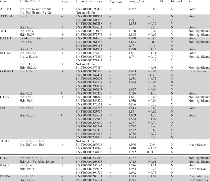For each gene, two or more gel bands are listed. Each band matches a set of Ensembl transcripts for which various MMBGX results are shown. The fourth column shows whether there is agreement in the relative direction of change in transcript use between MMBGX and the gel image. The fifth column gives the probability of differential transcript use, while the sixth column gives the fold change for each transcript. Transcripts with predicted expression close to zero in both conditions are marked as filtered. The concordance between the MMBGX results and the RT-PCR validation is shown in the right-most column. Genes above the thick line were significant in the Gardina workflow, while genes below it were not.

Altogether, 24 bands were scored by us. The MMBGX results for 10 bands agreed well with the RT-PCR, 9 were non-significant, 3 were inconclusive and 2 were contradictory. Three of the bands did not match any transcripts listed on the Ensembl database. Only the MMBGX results for two of the bands, both relating to ITGB4, contradicted the RT-PCR validation in direction of change. Note that the Gardina workflow did not pick up ITGB4 as a candidate for differential splicing since it was part of the eight previously reported genes (cf. Figure 12), suggesting that the microarray data contradicts the RT-PCR data for this gene.

Figure 12.

A schematic of the MMBGX validation of the colon cancer data set and its comparison to the Gardina workflow. Out of 168 genes in the Gardina workflow, 42 were validated by RT-PCR as were an additional eight genes picked because they had been reported in previous studies. Gel bands for 12 positively validated genes were provided by Gardina et al., nine from their workflow and three from previous studies. The MMBGX and Gardina workflow results for the 12 positively validated genes and 34 negatively validated genes are shown.

Out of the 50 genes tested, 34 produced negative RT-PCR results for differential splicing. Of these, 17 genes had incompatible Ensembl annotation. These probesets either mapped to an intron, an exon shared by all transcripts of a gene, a gene with only one isoform, a promoter exon or a poly-A termination exon. As such, these events could not be incorrectly called by MMBGX, illustrating one of the strengths of restricting the search to known isoforms. Out of the remaining 17 genes, only three, FAM44B, GBA and CDH11 were declared significant by MMBGX. However, in the case of CDH11 the significant result was due to only a small difference in the up-regulation of the two alternative isoforms (FC of 1.55 for ENST00000268603 and FC of 1.21 for ENST00000268602). This is shown in detail in Supplementary Table S1.

Comparison between MMBGX, COSIE and FIRMA

Finally, we analysed the data set using two recent exon-level methods, COSIE (19) and FIRMA (9), which have been shown to improve upon the original Splicing Index. We obtained COSIE presplicing indices and FIRMA scores for each exon-level probeset and calculated the P-values for a difference in means using paired t-tests. For each method, we estimated two thresholds for the P-values based on a false discovery rate (FDR) of 0.2 and 0.3 using Storey's; method (20). For each of the 12 positively validated genes for which gel images were provided, we checked whether the exon-probesets targeting the validated differentially spliced exons had P-values below the threshold. If so, the genes were declared true positives, otherwise they were declared false negatives. For the 36 negatively validated genes, we counted those with any probeset P-value below the threshold as false positives and the others as true negatives. From the results in Figure 12, we can see that in terms of the true negatives, COSIE and FIRMA gave equivalent results but that COSIE performed slightly better for detecting true positives. MMBGX outperformed both in terms of power, finding 7 out of the 12 positively validated genes, whereas for a similar level of false positives, COSIE only found 3. These results are shown in detail in Supplementary Tables S2 and S3.

To summarize, amongst the 46 genes tested by RT-PCR (the 12 positives where a gel image was provided and the 34 negatives), 38 MMBGX results agreed and 6 disagreed (where a gene with a ‘good’ result and no ‘contradictory’ results counts as an agreement), giving an error rate of 0.14. The Gardina workflow method agreed on 14 genes and disagreed on 32, giving an error rate of 0.73. Hence, the MMBGX results are much more consistent with the RT-PCR results, despite the fact that the candidates for RT-PCR testing were chosen on the basis of the Gardina workflow method. MMBGX also outperformed COSIE, which had an error rate of 0.26 (FDR < 0.2) and 0.50 (FDR < 0.3) and FIRMA, which had an error rate of 0.28 (FDR < 0.2) and 0.54 (FDR < 0.3). These results are shown in Figure 12.

DISCUSSION

Non-specific hybridization and probe-affinity effects

Our model treats non-specific hybridization at the probe level as exchangeable within groups of probes with similar GC content. Each GC content category k( j ) captures probe j's affinity effect through the means and variances of the log-scale background intensities, and . However, it has been shown—albeit in the case of RNA–DNA hybridizations on 3′ chips—that probe affinity effects depend not only on overall GC content but also on the precise positioning of each of the bases on an oligonucleotide (1). If a different predictor of affinity than GC content is preferred, it can be incorporated into MMBGX by binning the background probes according to this predictor and mapping the PM's; to the appropriate bin. Therefore, while in this article we used Affymetrix's; simple GC content-based scheme, more sophisticated schemes can be integrated into the models in a straightforward way.

Sequence-specific effects in Affymetrix microarrays have to date been modelled as part of the background noise by exploiting information in the MM probes on 3′-arrays or the background probes on whole-transcript arrays (e.g. GCRMA, PLIER, MMBGX). However, it is reasonable to assume that these effects apply not only to the non-specific hybridization component of the probe intensities, but also to the signal component. Some methods have included multiplicative probe effects (e.g. RMA) to account for systematic effects between probes, but these do not use the sequence information for each probe. In future work, we aim to refine our method by incorporating GC-specific affinity effects in the modelling of the probe-level signal as well as the non-specific hybridization.

Reliance on comprehensive transcript annotation

Transcript-level analysis relies on the comprehensiveness of the annotations used. If a transcript is highly abundant in a sample but is not targeted by a specific probeset, the signal from a different but similar transcript may be overestimated, yielding a false positive. In cases where an unknown real transcript is highly abundant in a sample and contains all the exons in a smaller Ensembl transcript, the Ensembl transcript acts as an unbiased proxy for the real transcript. Conversely, if an Ensembl transcript is more extensive than a real, unknown and highly abundant transcript, the Ensembl transcript acts as a downward-biased proxy due to its inclusion of unexpressed exons. Therefore, it is advisable to use MMBGX in conjunction with an effective exon-level method, such as COSIE, to ensure that novel events are not missed. At the time of writing, the human and mouse Exon arrays were found to target 52 743 and 40 420 Ensembl transcripts, respectively, and newly verified transcripts are being added on a regular basis. Thus, with each revision of Ensembl, the chance of being confounded by an unknown transcript is reduced. The rat genome, with only 34 006 known transcripts, has been less extensively annotated, so caution should be exercised when interpreting MMBGX results from rat data. Naturally, alternative sources of annotation may be used to construct the MMBGX probe–probeset structure files and interrogate a more extensive, although possibly less established, set of transcripts.

Comparison to methods for custom-built junction arrays and tiling arrays

Other methods have been developed that rely on custom-built arrays with junction probes and cannot straightforwardly be applied to Exon arrays. GenASAP estimates the expression of alternative isoforms uniquely distinguishable by inclusion or exclusion of a single predefined cassette exon (21). DECONV, like MMBGX, tries to disaggregate the signal at probes targeting multiple transcripts but requires arrays specifically designed to capture predefined gene structures (22). The principal advantage of using Exon arrays and MMBGX relative to custom junction arrays and these approaches is that, as improved transcript annotation becomes available, MMBGX may be incorporated into a re-analysis of the data without needing to redesign the array and repeat the experiment. More recently, ahierarchical Bayesian model (23) has been proposed to estimate isoform expression using tiling arrays. A very large number of arrays (91 in the case of 5-bp offsets along the human genome) are required for a single sample, however, which may make the approach impractical.

CONCLUSION

We have presented a fully hierarchical Bayesian model to estimate expression values from whole-transcript GeneChip microarrays. It is, to our knowledge, the first method to use the multi-mapping structure between probes and probesets to split the expression signal in a logical way and to model Exon array data at the transcript rather than the gene or exon level. MMBGX uses the rich transcriptional annotation on the Ensembl databases to detect and quantify the expression of alternative splice variants. With successive Ensembl releases, predictions can be updated and improved accordingly. Given the established importance of alternative splicing to the proteome (24), we hope that MMBGX will prove useful in characterizing the roles of alternative isoforms in different tissues and species during normal development and in disease.

SUPPLEMENTARY DATA

Supplementary Data are available at NAR Online.

FUNDING

EU (grant FP6-36495); BBSRC (grants BBG0003521 and BBC5196701). Funding for open access charge: BBSRC.

Conflict of interest statement. None declared.

REFERENCES

- 1.Naef F, Magnasco MO. Solving the riddle of the bright mismatches: labeling and effective binding in oligonucleotide arrays. Phys. Rev. E Stat. Nonlin. Soft Matter Phys. 2003;68(Pt 1):011906. doi: 10.1103/PhysRevE.68.011906. [DOI] [PubMed] [Google Scholar]
- 2.Wu Z, Irizarry RA, Gentleman R, Martinez-Murillo F, Spencer F. A model-based background adjustment for oligonucleotide expression arrays. J. Am. Stat. Assoc. 2004;99:909–917. [Google Scholar]
- 3.Turro E, Bochkina N, Hein A, Richardson S. BGX: a Bioconductor package for the Bayesian integrated analysis of Affymetrix GeneChips. BMC Bioinformatics. 2007;8:439. doi: 10.1186/1471-2105-8-439. [DOI] [PMC free article] [PubMed] [Google Scholar]
- 4.Affymetrix, Inc. Affymetrix GeneChip Exon Array Design. Technical report. 2005 http://www.affymetrix.com/support/technical/technotes/exon_array_design_technote.pdf. [Google Scholar]
- 5.Affymetrix, Inc. Affymetrix Guide to Probe Logarithmic Intensity Error (PLIER) Estimation. Technical report. 2005 http://www.affymetrix.com/support/ technical/technotes/plier_technote.pdf. [Google Scholar]
- 6.Affymetrix Inc. Affymetrix Exon Array Background Correction. Technical report. 2005 http://www.affymetrix.com/support/technical/whitepapers/exon_ background_correction_whitepaper.pdf. [Google Scholar]
- 7.Clark TA, Schweitzer AC, Chen TX, Staples MK, Lu G, Wang H, Williams A, Blume JE. Discovery of tissue-specific exons using comprehensive human exon microarrays. Genome Biol. 2007;8:R64. doi: 10.1186/gb-2007-8-4-r64. [DOI] [PMC free article] [PubMed] [Google Scholar]
- 8.Affymetrix Inc. Affymetrix Alternative Transcript Analysis Methods for Exon Arrays. Technical report. 2005 http://www.affymetrix.com/support/technical/whitepapers/exon_alt_ transcript_analysis_whitepaper.pdf. [Google Scholar]
- 9.Purdom E, Simpson KM, Robinson MD, Conboy JG, Lapuk AV, Speed TP. FIRMA: a method for detection of alternative splicing from exon array data. Bioinformatics. 2008;24:1707–1714. doi: 10.1093/bioinformatics/btn284. [DOI] [PMC free article] [PubMed] [Google Scholar]
- 10.Frigessi A, van deWiel MA, Holden M, Svendsrud DH, Glad IK, Lyng H. Genome-wide estimation of transcript concentrations from spotted cDNA microarray data. Nucleic Acids Res. 2005;33:e143. doi: 10.1093/nar/gni141. [DOI] [PMC free article] [PubMed] [Google Scholar]
- 11.Hein AMK, Richardson S, Causton HC, Ambler GK, Green PJ. BGX: a fully Bayesian integrated approach to the analysis of Affymetrix GeneChip data. Biostatistics. 2005;6:349–373. doi: 10.1093/biostatistics/kxi016. [DOI] [PubMed] [Google Scholar]
- 12.Flicek P, Aken BL, Beal K, Ballester B, Caccamo M, Chen Y, Clarke L, Coates G, Cunningham F, Cutts T, et al. Ensembl 2008. Nucleic Acids Res. 2008;36:D707–D714. doi: 10.1093/nar/gkm988. [DOI] [PMC free article] [PubMed] [Google Scholar]
- 13.Hein AMK, Richardson S. A powerful method for detecting differentially expressed genes from genechip arrays that does not require replicates. BMC Bioinformatics. 2006;7:353. doi: 10.1186/1471-2105-7-353. [DOI] [PMC free article] [PubMed] [Google Scholar]
- 14.Roberts GO, Rosenthal JS. Examples of Adaptive MCMC. 2006 http://www.probability.ca/jeff/ftpdir/adaptex.pdf. [Google Scholar]
- 15.Yates T, Okoniewski MJ, Miller CJ. X:map: annotation and visualization of genome structure for Affymetrix exon array analysis. Nucleic Acids Res. 2008;36:D780–D786. doi: 10.1093/nar/gkm779. [DOI] [PMC free article] [PubMed] [Google Scholar]
- 16.Bolstad BM, Irizarry RA, Astrand M, Speed TP. A comparison of normalization methods for high density oligonucleotide array data based on variance and bias. Bioinformatics. 2003;19:185–193. doi: 10.1093/bioinformatics/19.2.185. [DOI] [PubMed] [Google Scholar]
- 17.Irizarry RA, Hobbs B, Collin F, Beazer-Barclay YD, Antonellis KJ, Scherf U, Speed TP. Exploration, normalization, and summaries of high density oligonucleotide array probe level data. Biostatistics. 2003;4:249–264. doi: 10.1093/biostatistics/4.2.249. [DOI] [PubMed] [Google Scholar]
- 18.Gardina PJ, Clark TA, Shimada B, Staples MK, Yang Q, Veitch J, Schweitzer A, Awad T, Sugnet C, Dee S. Alternative splicing and differential gene expression in colon cancer detected by a whole genome exon array. BMC Genomics. 2006;7:325. doi: 10.1186/1471-2164-7-325. [DOI] [PMC free article] [PubMed] [Google Scholar]
- 19.Gaidatzis D, Jacobeit K, Oakeley EJ, Stadler MB. Overestimation of alternative splicing caused by variable probe characteristics in exon arrays. Nucleic Acids Res. 2009 doi: 10.1093/nar/gkp508. 10.1093/nar/gkp508 [Epub ahead of print] [DOI] [PMC free article] [PubMed] [Google Scholar]
- 20.Storey JD. A direct approach to false discovery rates. J. Roy. Stat. Soc. Ser. B (Stat. Methodol.) 2002;64:479–498. [Google Scholar]
- 21.Shai O, Morris QD, Blencowe BJ, Frey BJ. Inferring global levels of alternative splicing isoforms using a generative model of microarray data. Bioinformatics. 2006;22:606–613. doi: 10.1093/bioinformatics/btk028. [DOI] [PubMed] [Google Scholar]
- 22.Wang H, Hubbell E, Hu JS, Mei G, Cline M, Lu G, Clark T, Siani-Rose MA, Ares M, Kulp DC, et al. Gene structure-based splice variant deconvolution using a microarray platform. Bioinformatics. 2003;19(Suppl 1):i315–i322. doi: 10.1093/bioinformatics/btg1044. [DOI] [PubMed] [Google Scholar]
- 23.Zheng S, Chen L. A hierarchical bayesian model for comparing transcriptomes at the individual transcript isoform level. Nucleic Acids Res. 2009;37:e75. doi: 10.1093/nar/gkp282. [DOI] [PMC free article] [PubMed] [Google Scholar]
- 24.Garcia-Blanco MA, Baraniak AP, Lasda EL. Alternative splicing in disease and therapy. Nat. Biotechnol. 2004;22:535–546. doi: 10.1038/nbt964. [DOI] [PubMed] [Google Scholar]
Associated Data
This section collects any data citations, data availability statements, or supplementary materials included in this article.