Comparative study on ChIP-seq data: normalization and binding pattern characterization

Abstract

Motivation: Antibody-based Chromatin Immunoprecipitation assay followed by high-throughput sequencing technology (ChIP-seq) is a relatively new method to study the binding patterns of specific protein molecules over the entire genome. ChIP-seq technology allows scientist to get more comprehensive results in shorter time. Here, we present a non-linear normalization algorithm and a mixture modeling method for comparing ChIP-seq data from multiple samples and characterizing genes based on their RNA polymerase II (Pol II) binding patterns.

Results: We apply a two-step non-linear normalization method based on locally weighted regression (LOESS) approach to compare ChIP-seq data across multiple samples and model the difference using an Exponential-Normal^K mixture model. Fitted model is used to identify genes associated with differential binding sites based on local false discovery rate (fdr). These genes are then standardized and hierarchically clustered to characterize their Pol II binding patterns. As a case study, we apply the analysis procedure comparing normal breast cancer (MCF7) to tamoxifen-resistant (OHT) cell line. We find enriched regions that are associated with cancer (P < 0.0001). Our findings also imply that there may be a dysregulation of cell cycle and gene expression control pathways in the tamoxifen-resistant cells. These results show that the non-linear normalization method can be used to analyze ChIP-seq data across multiple samples.

Availability: Data are available at http://www.bmi.osu.edu/~khuang/Data/ChIP/RNAPII/

Contact: taslim.2@osu.edu; khuang@bmi.osu.edu

Supplementary information: Supplementary data are available at Bioinformatics online.

1 INTRODUCTION

Next-generation high-throughput ChIP sequencing technology (ChIP-seq) is becoming the preferred method for studying protein–DNA bindings. It allows researchers to sequence tens of millions of DNA fragments in a single experiment. It has been shown to produce high-quality, high-specificity and high-sensitivity data and it is also a cost-effective approach for mapping genome-wide protein–DNA interaction (Johnson et al., 2007). One of the earlier method to study DNA binding proteins on the whole genome is ChIP-chip (Horak and Snyder, 2002; Ren et al., 2000), a procedure which involves immunoprecipitation of DNA using protein-specific antibody and then hybridizing it to a genomic tiling array. Compared with ChIP-chip, experiments done in ChIP-seq does not need to worry about errors associated with cross-hybridization and the noisy polymerase chain reaction (PCR) amplification process. In ChIP-seq, the protein-bound DNA fragments (tags) are sequenced by reading up to 72 nt from both ends. Parallel sequencing is then performed to uniquely align these sequences back to the genome producing tens of millions mapped fragments. Various procedures such as sample preparation, tags amplification, base calling, image processing and sequence alignment are needed to massively sequence the short tags and get their unique genomic location. Even though ChIP-seq data are less prone to error, the large amount of data being produced and bias generated by various procedures mentioned above pose new challenges in analyzing ChIP-seq data. Innovative computational and statistical approaches are therefore required to separate biological signal from noise. One of them is data normalization which is very critical when comparing results across multiple samples. Normalization is certainly needed to identify any systematic error and bias that are not due to biological signal. Under ideal environment where experiments are run in a perfect condition without even the slightest error, we would expect all differences to be associated with the biological changes in the samples. However, as with all experiments there are some factors that cannot be controlled which bias the results and thus creating differences that do not reflect the biological conditions. The purpose of normalization is to identify such systematic errors and eliminate them to reveal the true biological signals.

Here, we present a non-linear normalization method for ChIP-seq data to reveal biological differences across samples. To the best of our knowledge, normalization methods for ChIP-seq data are very limited. Although several papers have been published to analyze data generated using ChIP-seq technology, many simply normalized their data against the tags sequencing depth (Feng et al., 2008; Ji et al., 2008; Kharchenko et al., 2008; Xu et al., 2008; Zhang et al., 2008). This method is commonly used to normalize serial analysis of gene expression (SAGE) library, which is a collection of thousands of small DNA fragments. It is based on the assumption that the total number of DNA bindings would be similar in different cell types under different biological conditions. The number of fragments aligned is normalized using the total number of matched fragments in each sample. Hence, the normalized data will have equal number of tags across samples. While normalizing against the tags sequencing depth enable comparison across samples, it does not remove systematic errors. For example, if an equipment is not calibrated correctly in one sample causing a systematic error in one particular experiment, then comparison between this sample with the others will incorrectly detect the error as the effect of different biological conditions. Recently, Rozowsky et al. (2009) address this problem by using a linear scaling factor. They exclude potential peaks from normalization method by comparison with input-DNA control and then scaled the data by a linear factor. Here, we avoid making linearity assumption by using a non-parametric regression to normalize ChIP-seq data.

Based on the assumption that the mean of non-differential tags will be zero, we introduce a two-stage normalization method for ChIP-seq data and apply it to identify genes with enriched polymerase II (Pol II) regions in breast cancer MCF7 cell line under different conditions and OHT cell line, as a case study.

17 β-estradiol (E2)-induced and tamoxifen-resistant MCF7 cell lines are chosen for case study, since the hormonal exposure is the best characterized risk factor for breast cancer. Previous evidence supports the association of estrogen exposure with the increased risk of breast cancer (Hulka et al., 2004). The distribution of estrogen receptor (ERα) profile indicates a highly dynamic and complicated regulation network (Carroll et al., 2006; Lin et al., 2007). The data from ChIP-seq will be very helpful for fully characterizing and understanding estrogen regulatory network. Tamoxifen is one of selective ER modulators (SERMs) and is widely used to block ERα function for breast cancer treatment (Osborne and Schiff, 2005). However, this endocrine therapy is limited by the onset of tamoxifen resistance. Delineating the changed architectures of ERα regulation network in tamoxifen resistance cells may provide direct and useful information of tamoxifen resistance.

This article is organized as follows: ChIP-seq data processing, normalization, statistical analysis and clustering methods are proposed in Section 2; Analysis on data from normal breast cancer (MCF7) cell line after E2 treatment and tamoxifen-resistant subline (OHT-MCF7) are presented in Section 3; and finally, discussion and future directions are presented at the end of the article.

2 METHODS

Our ChIP-seq experiments are done on breast cancer cell lines comprising three different experiments: MCF7 control, MCF7 + E2 treatment and OHT (tamoxifen-resistant subline OHT-MCF7). The aim of this biological problem is to find differential areas of enrichment by comparing the treatment samples (i.e. OHT and MCF7 + E2) with the MCF7 control as a reference and uncover the biological characteristics of tamoxifen-resistant and E2 treatment in breast cancer cells. To accomplish this objective, we first normalized the data to eliminate the effects of background noise, base calling, image processing error and any other systematic errors. Next, we applied a model-based classification technique to find genes associated with the differential binding quantity. Finally, we clustered the significant genes profile based on their Pol II binding patterns. A summary of the workflow is shown in Figure 1. In this section, we provide brief descriptions of data used, the normalization method followed by the finite mixture modeling technique and hierarchical clustering algorithm.

Fig. 1.

Flow chart of the processes done in this article.

2.1 Breast cancer data

MCF7 human breast cancer cells (American Type Culture Collection, Manassas, VA, USA) and tamoxifen-resistant MCF7 cells (OHT) were maintained as described by Fan et al. (2006). Both MCF7 and OHT were treated with E2 (10⁻⁸mol/l) for 3 h. For each immunoprecipitation, cells were cross-linked with 1% formaldehyde for 10 min and sonicated to fragment the chromatin to a size range of 200 bp to 1 kb. Chromatin fragments were then immunoprecipitated with 10 μg of antibodies against Pol II and ERα (sc-899 X and sc-8005 X, Santa Cruz, CA, USA). After immunoprecipitation, washing and elution, ChIP DNA was purified by phenol:chloroform:isoamyl alcohol and solubilized in 70 μl of water. Then Illumina library was constructed and sequenced with Illumina/Solexa Genome Analyzer (Michael Smith Genome Sciences Centre, Vancouver, Canada).

2.2 Mapping DNA fragments and determining putative binding sites

Given a library of short DNA fragments generated from ChIP-seq experiments, the first step was to map these tags back onto the genome to obtain their locations and orientations. We used ELAND (Cox, unpublished software), provided by Illumina, to align these short sequence reads to the genome allowing up to two mismatches. After the realignment stage, we have fragment counts in each genomic location. In our ChIP-seq experiments, a tag is sequenced by reading up to 36 nt from both ends of the DNA fragment. Hence, the real binding sites (i.e. the center of the corresponding DNA sequence) is unknown. In order to determine the putative binding sites, several ChIP-seq-based techniques shift all tags d/2 toward its orientation, where d is the distance between the peak in the forward and reverse strand (Kharchenko et al., 2008; Xu et al., 2008; Zhang et al., 2008). Unlike most DNA binding proteins which bind to a distinct site, Pol II binds throughout the promoter, upstream and downstream regions of the activated gene. Thus, in our analysis, it is unnecessary to do any shifting. Furthermore, since we are interested in characterizing the differential binding patterns in multiple samples, the effect of shifting would be negligible.

2.3 Normalization

In the analysis of any comparative experiments, there is a need to normalize the data to remove bias and enable comparison across multiple samples. ChIP-seq experiments like many other experiments are prone to systematic errors. Under ideal (error-free) environment, we would expect no difference in the measurement of two experiments under the same biological condition. However, there are intensities measurement error and other effects that contribute to bias in the experiments, making the difference to be non-zero. For example, in ChIP-seq experiment, during the base calling stage, fluorescence intensities will decrease over time adding bias to the measurement. Hence, we would want to normalize the data to ensure the mean of non-differential sites are zero and that the effect of bias does not overwhelm the data itself. Also, we want to make sure that there is equal variance across the samples. Having non-constant variance will influence methods to find differentially enriched regions in the areas which have larger spread.

Although several approaches have been proposed to analyze ChIP-seq data, many normalized their data simply by using the total number of fragments in each sample or using the sequencing depth (Feng et al., 2008; Ji et al., 2008; Kharchenko et al., 2008; Xu et al., 2008; Zhang et al., 2008). This straightforward method of normalization scales the raw data by a constant factor. This method is prone to bias caused by unequal variance in different genomic regions. Rozowsky et al. (2009) scales the raw data using a linear factor; however, such a linearity assumption is unrealistic in many applications. In this article, we implement a non-linear normalization method using locally weighted polynomial least square regression (Cleveland, 1988) to estimate a LOESS smoother of the mean and variance of the observed data. Compared with the straightforward method of using the sequencing depth, we find the LOESS normalization method better equipped in removing the effect of bias and systematic errors. This normalization technique has been applied successfully on cDNA microarray datasets (Dean and Raftery, 2005).

Let x_ij be the Pol II binding quantity for bin i (i = 1,…, n), where n is the total number of bins in a chromosome and j = 1, 2 refers to control (reference) and treatment samples, respectively. In our application, we use bins of size 1K nt, i.e. x_ij is the sum of fragments counts that are mapped between location (i − 1)×1000 and i× 1000 + 1 in sample j. Bin size of 1K nt is chosen to balance between the number of data points and resolution. The normalization process is a two-step procedure. First, the fitted values are estimated by regressing the observed difference on the mean counts:

(1)

where x_i1 and x_i2 are the observed fragment counts in control and treatment samples as described previously. Ŷ_mean is the fitted value from regressing the difference on the mean counts. Then the fitted values are subtracted from the observed difference counts as follows:

(2)

Thus, D_meannorm is the data after correction with respect to the mean. As shown in Figure 2b, after this step, the average of the mean-normalized data is close to zero (indicated by the green/dash-dot line). Instead of modeling log-ratios, as in Dean and Raftery (2005), we use the binding quantity of each sample directly (i.e. using difference counts). By using the fragment counts directly, it enables us to differentiate sites with the same log ratios, but vastly different magnitude in their individual binding quantities. Furthermore, in gene expression data, a threshold is commonly applied in the preprocessing step to filter out low values before taking the log-ratios of the intensities. However, in ChIP-seq experiments, zeros are meaningful (i.e. there is nothing that binds to the regions). Hence, we do not want to apply a threshold to filter out zero-count as doing so would lead to loss of information.

Fig. 2.

An example of the normalization process applied to the binding quantity difference between MCF7 control and MCF7 + E2 breast cancer data on Chromosome 1. (a) Raw data with clear bias towards the positive direction; (b) data normalized with respect to the mean; (c) data normalized with respect to both mean and variance (x-axis is zoomed-in). Green (dash-dot) and magenta (dashed) lines represent the LOESS smoother line with respect to the mean and variance, respectively. Red (dotted) line represents the zero-difference line. For color version of the figure see Bioinformatics online.

In our application, we use a loess span of 60% to get a good normalization with respect to the mean. At this step, we generally have adjusted bias with respect to the mean but not the spread (see Fig. 2b). In the second step, the moving mean absolute deviation Ŷ_var is estimated by regressing the absolute of the mean-normalized difference (estimated in the first step) on the absolute mean counts:

(3)

As indicated by the LOESS line (magenta/dashed line) on Figure 2b, the variability appears to increase as the mean becomes larger. In order to normalize the variance, the mean-normalized difference counts [Equation (2)] is divided by the estimated mean of absolute deviation Ŷ_var

(4)

We get a good result using 10% of neighborhood points (span = 10%) to estimate the running mean absolute standard deviation. The two-step normalization process provides a nice transformation leading to homoscedastic variance (Fig. 2c).

2.4 Finite mixture model for differential genes selection

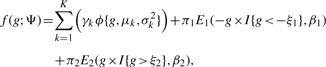
After normalization, we apply methods to find genes associated with differential binding quantity. One of the earliest method is the rule of two (Schena et al., 1996) in which genes with ratios greater than two or less than a half are considered to be differential. Although this method is very simple to use, it is not based on any statistical principles. Here, we fit a finite mixture model to the normalized data and perform model-based classification to identify genes associated with enrichment regions. In the mixture model, we assume that the data comes from three (non-differential, positive- and negative-differential) groups. The non-differential regions are assumed to come from a mixture of K-component normal distributions, where K is unknown and needs to be estimated from the data. The positive- and negative-differential regions are assumed to follow exponential and the mirror of exponential distributions, respectively. Khalili et al. (2009) gives a detailed description of the finite mixture model and uses the model to find differentially expressed genes and differentially methylated probes in CpG islands. The choice of these distributions to represent the data is based on the observation that the expected value of non-differential, positive- and negative-differential binding sites are zero, positive and negative values, respectively. The data d_i ∈ D_meanvarnorm are grouped based on known gene regions to determine areas of enrichment associated with a gene. Denote G_w as the normalized fragments difference of gene w. Each gene region (w) is defined according to genes annotation in RefSeq database. Let W equals to the total number of genes in RefSeq. Then for each gene region w, we have G_w = ∑d_i, ∀i ∈ R where R is the sets of fragments within a gene region w ∈ {1,…, W}. We then fit an empirical distribution based on G_w, the normalized difference in a gene region. Suppose f(g) is the unknown density function of the observed data G_w. We approximate the unknown function as a mixture of K-normal components and exponential components:

(5)

where Ψ is a vector of unknown parameters of the mixture distributions; ϕ{.} denotes the Normal density function; I{.} is an indicator function that equals to 1 if the condition specified in {} is satisfied, and 0 otherwise; ξ₁, ξ₂ > 0 are the location parameters which are assumed to be known. In practice, and may be used as estimates of ξ₁ and ξ₂. The first K components denote the proportion of data and are modeled by normal densities function with mean μ_k and variance σ²_k. It is designed to capture the non-differential binding sites, with parameter γ_k interpreted as the proportion of non-enriched regions. The other two components use location-exponential density function to represent the positive- and negative-differential areas of enrichments. The parameters π₁ and π₂ denote the proportion of positive- and negative-differential binding density, respectively.

In order to find the best model to represent the observed data, a set of optimal parameters Ψ* is estimated by maximizing the likelihood function using Expectation-Maximization (EM) algorithm for a fixed K. Then akaike's information criteria (AIC) (Akaike, 1973) is used to select K that provides the best explanation of the data. Local false discovery rate (fdr) is calculated to determine whether g_w, the normalized fragment counts difference in the region associated with gene w is significantly enriched (fdr(g_w)≤z₀):

(6)

In our application, we set z₀ = 0.1.

A common concern when fitting a mixture model is the issue of identifiability. In our approach, since we assume all normal, exponential and its mirror components to capture genes with non-differential and positive/negative-differential binding sites, these three components are identifiable. In fact, it has been shown that finite mixture of exponential and normal components are generically identifiable (Teicher, 1961, 1963).

2.5 Clustering Pol II binding profiles

Although Pol II can form a distinct binding site around the transcription start site (TSS), it also binds and proceeds along the promoter regions, the 5′ and 3′ end regions and the downstream regions of activated genes. Thus, it is of interest to investigate the Pol II binding patterns, which will provide new insight on the dynamics of gene transcription by Pol II. Here, we cluster the genes which are found to have significantly different binding sites and investigate whether distinct binding patterns exist. To cluster the gene profiles, we first filter out all the fragments associated with introns and only retain the ones falling into the exons regions since Pol II mainly acts on the exon region for transcription. After filtering out the introns, we denote §_w as the normalized tag counts in the exons regions for gene w. Genes length are standardized to enable genome-wide profiling. The interpolation is done with optimum interpolators designed using direct form II transposed filter (Oetken et al., 1975). As a result of the interpolation, all genes have the same length artificially. We then perform hierarchical clustering of §_w to group genes based on their Pol II binding patterns. Similarity distance is calculated using Pearson's linear correlation coefficient. Genes within a group have similar binding patterns with each other.

3 RESULTS

3.1 Effects of E2 treatment on MCF7 cell

First, we demonstrate the normalization and statistical modeling methods described above on the study comparing the Pol II binding quantities between the MCF7 and E2-treated MCF7 cells. Figure 2 shows the normalization process with MCF7 as the reference. By normalizing the data with respect to both mean and variance, we are able to spread the points more evenly around zero and reduce the systematic error (Fig. 2c) which is essential for eliminating bias caused by unequal variance and outliers. The normalized fragments are then grouped by their corresponding gene regions. Next, we fit the normalized difference with the mixture model using EM algorithm. The EM algorithm was re-initialized 1125 times to prevent it from getting stuck in a local optimum. Each time the EM step is terminated either after 2000 iterations or when the improvement on the likelihood function is not greater than 10⁻¹⁶. Figure 3 shows the best mixture model fitting the data for the whole genome, which is a mixture of two exponential and three normal components.

Fig. 3.

The fit of the best mixture model on the normalized MCF7 versus MCF7+E2 data. The optimal mixture model and its individual components are plotted. Blue (solid) line represents the best mixture model (mixture of two exponential and three normal components) imposed on the histogram of the normalized difference of the binding quantity. Black (dashed), brown (dotted) and green (dot-dash) lines represent normal components with (μ₁ = 5; σ₁ = 8), (μ₂ = 9; σ₂ = 26), (μ₃ = 19; σ₃ = 63), respectively. Red (long-dash) and magenta (two-dash) represent exponential components with β₁ = 127 and β₂ = 112, respectively. For color version of the figure see Bioinformatics online.

Subsequently, we apply the model-based classification to find genes associated with differential binding sites using fdr. We classify a binding site as significant when its fdr < 0.1. Since we group binding sites according to their respective gene regions, the gene with different Pol II binding density is also significant. We refer to these genes as significant genes. In the MCF7+E2 cells (Table 1), 448 genes are found to be significant. The results are consistent with previous findings. For instance, PGR and GREB1 have been reported as ER target genes that are upregulated and MCF7 + E2 cells have been shown to have more genes upregulated than downregulated after E2 treatment (Feng et al., 2008; Lin et al., 2004). The list of significant genes is provided in the Supplementary Material.

Table 1.

A summary of significant genes identified from MCF7+E2 and OHT with MCF7 as a reference

	Comparison with MCF7 control
	MCF7 + E2	OHT	(MCF7 + E2) ∩ OHT
No. genes with decreased binding	184	373	62
No. genes with increased binding	264	282	41
No. of known genes (RefSeq)	18 364

3.2 Comparison of Pol II binding between MCF7 and OHT cells

We then applied the same methods comparing the tamoxifen-resistant OHT cells with the MCF7 and the results are summarized in Table 1. In the OHT cells, there are more (655 in total) significant genes than those in the MCF7 + E2 cells. In particular, the number of downregulated genes in OHT (373) is more than doubled the ones found in MCF7 + E2 cells (184). This may help to explain the mechanism of tamoxifen-resistance in the OHT cells. Therefore, we carried out functional analysis on the 311 genes that are uniquely associated with decreased Pol II bindings in OHT using Ingenuity Pathway Analysis (IPA, http://www.ingenuity.com), which calculates the P-values using right-tailed Fisher's exact test. Cellular growth and proliferation, cellular movement and embryonic development are the top functional groups and cancer is the top disease associated with these genes. In addition, we identified a group of highly connected subset of 100 genes that are enriched with functions including gene expression (38 genes), cell-cycle control (19 genes) and cell death control (39 genes) as shown in Figure 4. Furthermore, Gene Ontology (GO) enrichment analysis also identifies positive regulation of anti-apoptosis as significant (P < 0.0052, using hypergeometric test). Our findings thus suggest a dysregulation of cell-cycle and gene expression control pathways as well as apoptosis control in the tamoxifen-resistant cells. The detailed GO results can be found in the Supplementary Table 2 and Supplementary Figure 4.

Fig. 4.

top 10 functional groups identified by IPA for the 100 highly connected genes that show decreased Pol II binding quantities in OHT cells but not in E2-treated MCF7 cells. The blue bar indicates the minus logarithm (base 10) of the P-values for the Fisher's exact test. The threshold line indicating P < 0.05. For color version of the figure see Bioinformatics online.

3.3 Modulation of Pol II binding patterns

Different biological conditions not only lead to difference in Pol II binding quantities, but they can also induce changes in Pol II binding dynamics and patterns on the genes. ChIP-seq for the first time allows us to study such changes which may lead to a new direction in cancer research. To study this, we applied hierarchical clustering to the 448 significant genes found in MCF7 + E2 based on their Pol II binding patterns in MCF7 (Fig. 5a) and MCF7 + E2 (Fig. 5b), respectively. In E2-treated MCF7 cells, 167 genes show high binding near their TSS, 51 genes show enriched binding at the 3′ end and 24 genes exhibit high binding at both 5′ and 3′ ends. Eighty-five genes display high activities mostly in the first half of their gene regions and 77 genes exhibit high areas of enrichment in the second half of their gene regions. We see similar clustering for the MCF7 control. In particular, out of the 136 genes with high binding near the TSS, 89 genes also display high binding near TSS after E2 treatment (Fig. 6a). Alternative promoters of human genome, especially downstream promoter in E2-induced genes close to 3′-terminus of the gene has also been reported in Singer et al. (2008) using a custom promoter tiling array.

Fig. 5.

Hierarchical clustering of genes associated with differential binding sites in MCF7 and MCF7 + E2 cell lines and their associated Pol II binding patterns. (a) Binding patterns in MCF7 control and (b) binding patterns in MCF7 + E2. Red and blue color on the heatmap represent high- and low-binding quantity, respectively. Colored clusters indicate the different grouping based on their Pol II binding patterns. Genes in yellow cluster show high binding near their 3′ end. Cyan clustered genes show high binding around their 5′ end. Genes in green cluster tends to have high binding anywhere along the 3′ and 5′ ends. The genes clustered in both heatmap are identical.

Fig. 6.

A diagram showing the number of genes in (a) cluster which display high binding at 5′ end and (b) cluster which display high binding at 3′ end. For color version of the figure see Bioinformatics online.

Next, we cluster the 655 significant genes found in OHT [Supplementary Fig. 1a for patterns in MCF7 cells and Fig. 1b for OHT cells]. There are 334 genes and 358 genes displaying high bindings at their 5′ end in tamoxifen-resistant cell line and in normal breast cancer cells, respectively, and 188 genes are shared by the two groups (Fig. 6a). This observation implies that the Pol II binding pattern is more severely modulated in OHT than in MCF7 + E2. Comparing these list of genes in OHT and MCF7 + E2 cells, we find 125 genes displaying high bindings at their 5′ end only in OHT. Functional and GO analysis show that 95 of these genes are involved in protein bindings (details shown in Supplementary Table 1 and the Supplementary Fig. 3). The list of genes associated with increased/decreased bindings and genes associated with high-binding patterns at 5′ and 3′ ends are provided in the Supplementary Material.

4 DISCUSSION AND FUTURE WORK

ChIP-seq is a new technique which has the potential of replacing the ChIP-chip technology in studying protein–DNA binding. Recently, it has been noticed that comparative study is necessary to adequately use ChIP-seq data and therefore normalization is a key step in interpreting the data. Here, we present a two-step non-linear normalization method based on locally weighted regression (LOESS) to analyze ChIP-seq data across multiple samples in which the differences are normalized with respect to the estimated moving mean and variance. This normalization method can eliminate non-linear noise and bias without making any prior assumption about the shape of the noise. In addition, we apply a model-based approach to identify genomic regions with statistically significant changes in protein binding quantities between the normalized data. Although this normalization method is applied to ChIP-seq data without any replicates, it can also accommodate data with biological replicates.

We demonstrate the applicability of the normalization algorithm by interpreting the biological signals associated with estrogen-induced changes in Pol II binding quantity in normal breast cancer cells (MCF7) and comparing it with its tamoxifen-resistant cells (OHT). We perform data normalization and fit an Exponential-Normal^K finite mixture model on the normalized data to select genes with significant Pol II binding densities between the samples. The results on MCF7 cells are consistent with previous findings, while experimental validation of certain selected genes on changes related to the OHT cells are planned. The statistical analysis also allows us to focus on the selected genes to further study their Pol II binding patterns using hierarchical clustering. This provides a novel angle of investigating the effects of drugs and disease states on transcription regulation and may lead to a new direction in cancer research. Our current results reveal new insight on the dynamics of Pol II-mediated gene transcription and its regulation in MCF7 and OHT cells. We plan to extend the analysis to include miRNA regions, intron regions and a larger pool of genes by relaxing the threshold in the mixture step. In addition, we propose to carry out new experiments on studying the modulation of the dynamics of Pol II using synchronized cell culture. Then the same procedure can be scaled up easily and applied to analyze these genomic regions including non-coding RNAs.

As a comparison, we applied the sequence depth normalization approach which is a constant adjustment on the same datasets. The scaling factor is very close to one and thus the effect of the sequence depth normalization is very minimal. As shown in the Supplementary Figure 2, the green (dot-dashed) and the magenta (dashed) line indicate that the normalized data is still biased toward positive direction and have unequal variance. In contrast, the two-step LOESS normalization is correcting for both mean and variance making the normalized data to have mean around zero and homoscedastics (Fig. 2c). Moreover, since LOESS is a locally weighted smoothing function (i.e. more weights are given to points nearby and less weight to points further away), it is more robust to outliers.

To gauge the utility of our approach, we used CisGenome (Ji et al., 2008) on MCF7 versus MCF7 + E2 and chose fdr ≤ 0.1 as a cutoff to find genes associated with differential binding sites and compare them with our findings. Of the 448 genes that we found to be associated with differential bindings, 167 of them are also found by CisGenome. This is indicative that the programs are able to identify common features despite using different approaches. On the other hand, there are genes found by one of the two programs singularly, which appears to illustrate the different strengths of the programs in uncovering particular genes with differential binding patterns. However, future work is warranted for more definitive conclusion. We further caution that all these algorithms should be considered as a first-pass attempt to identify differential binding sites and both algorithms appear to complement each other to provide a more complete classification.

In our approach, we assume that the majority of the genes are not associated with differential binding sites between the reference and the treatment samples. This assumption is satisfied for applications in which the difference between the samples (i.e. the effects of a treatment) are not expected to influence a large proportion of binding sites such as ChIP-seq studies on RNA Pol II, histone markers, FoxA1 and ERα (Welboren et al., 2009; Zhang et al., 2008). However, if the difference between the total number of sequenced fragments from each sample is large such as in a knock-out gene experiment, it may be recommendable to extend the two-step normalization method described above to a three-step normalization procedure. In the first step, the raw data are normalized with respect to the sequence depth followed by the LOESS normalization approach with respect to mean and variance.

Funding: NCI ICBP (grant U54CA113001, partially); the PhRMA Foundation Research Starter Grant in Informatics (partially); the Ohio State University Comprehensive Cancer Center (partially).

Conflict of Interest: none declared.

REFERENCES

- Akaike H. International Symposium on Information Theory. 2nd. Armenian SSR: Tsahkadsor; 1973. Information theory and an extension of the maximum likelihood principle; pp. 267–281. [Google Scholar]
- Carroll J, et al. Genome-wide analysis of estrogen receptor binding sites. Nat. Genet. 2006;38:1289–1297. doi: 10.1038/ng1901. [DOI] [PubMed] [Google Scholar]
- Cleveland WS. Locally-weighted regression: An approach to regression analysis by local fitting. J. Am. Stat. Assoc. 1988;85:596–610. [Google Scholar]
- Dean N, Raftery AE. Normal uniform mixture differential gene expression detection for cDNA microarrays. BMC Bioinformatics. 2005;6:173. doi: 10.1186/1471-2105-6-173. [DOI] [PMC free article] [PubMed] [Google Scholar]
- Fan M, et al. Diverse gene expression and DNA methylation profiles correlate with differential adaptation of breast cancer cells to the antiestrogens tamoxifen and fulvestrant. Cancer Res. 2006;66:11954–11966. doi: 10.1158/0008-5472.CAN-06-1666. [DOI] [PubMed] [Google Scholar]
- Feng W, et al. A poisson mixture model to identify changes in RNA polymerase II binding quantity using high-throughput sequencing technology. BMC Genomics. 2008;9(Suppl. 2):S23. doi: 10.1186/1471-2164-9-S2-S23. [DOI] [PMC free article] [PubMed] [Google Scholar]
- Horak CE, Snyder M. ChIP-chip: a genomic approach for identifying transcription factor binding sites. Methods Enzymol. 2002;350:469–483. doi: 10.1016/s0076-6879(02)50979-4. [DOI] [PubMed] [Google Scholar]
- Hulka B, et al. Steroid hormones and risk of breast cancer. Cancer. 2004;74(Suppl. 3):1111–1124. doi: 10.1002/1097-0142(19940801)74:3+<1111::aid-cncr2820741520>3.0.co;2-l. [DOI] [PubMed] [Google Scholar]
- Ji H, et al. An integrated software system for analyzing ChIP-chip and ChIP-seq data. Nat. Biotechnol. 2008;26:1293–1300. doi: 10.1038/nbt.1505. [DOI] [PMC free article] [PubMed] [Google Scholar]
- Johnson DS, et al. Genome-wide mapping of in vivo protein-DNA interactions. Science. 2007;316:1441–1442. doi: 10.1126/science.1141319. [DOI] [PubMed] [Google Scholar]
- Khalili A, et al. A robust unified approach to analyzing methylation and gene expression data. Comput. Stat. Data Anal. 2009;53:1701–1710. doi: 10.1016/j.csda.2008.07.010. [DOI] [PMC free article] [PubMed] [Google Scholar]
- Kharchenko PVV, et al. Design and analysis of ChIP-seq experiments for DNA-binding proteins. Nature Biotechnol. 2008;26:1351–1359. doi: 10.1038/nbt.1508. [DOI] [PMC free article] [PubMed] [Google Scholar]
- Lin C-Y, et al. Discovery of estrogen receptor alpha target genes and response elements in breast tumor cells. Genome Biol. 2004;5:R66. doi: 10.1186/gb-2004-5-9-r66. [DOI] [PMC free article] [PubMed] [Google Scholar]
- Lin CY, et al. Whole-genome cartography of estrogen receptor alpha binding sites. PLoS Genet. 2007;3:e87. doi: 10.1371/journal.pgen.0030087. [DOI] [PMC free article] [PubMed] [Google Scholar]
- Oetken G, et al. New results in the design of digital interpolators. IEEE Trans. Acoust. Speech Signal Process. [see also IEEE Trans. Signal Process.] 1975;23:301–309. [Google Scholar]
- Osborne CK, Schiff R. Estrogen-receptor biology: Continuing progress and therapeutic implications. J. Clin. Oncol. 2005;23:1616–1622. doi: 10.1200/JCO.2005.10.036. [DOI] [PubMed] [Google Scholar]
- Ren B, et al. Genome-wide location and function of DNA binding proteins. Science. 2000;290:2306–2309. doi: 10.1126/science.290.5500.2306. [DOI] [PubMed] [Google Scholar]
- Rozowsky J, et al. Peakseq enables systematic scoring of ChIP-seq experiments relative to controls. Nat. Biotechnol. 2009;27:66–75. doi: 10.1038/nbt.1518. [DOI] [PMC free article] [PubMed] [Google Scholar]
- Schena M, et al. Parallel human genome analysis: microarray-based expression monitoring of 1000 genes. Proc. Natl Acad. Sci. USA. 1996;93:10614–10619. doi: 10.1073/pnas.93.20.10614. [DOI] [PMC free article] [PubMed] [Google Scholar]
- Singer G, et al. Genome-wide analysis of alternative promoters of human genes using a custom promoter tiling array. BMC Genomics. 2008;9:349. doi: 10.1186/1471-2164-9-349. [DOI] [PMC free article] [PubMed] [Google Scholar]
- Teicher H. Identifiability of mixtures. Ann. Math. Stat. 1961;32:244–248. [Google Scholar]
- Teicher H. Identifiability of finite mixtures. Ann. Math. Stat. 1963;34:1265–1269. [Google Scholar]
- Welboren W-J, et al. ChIP-Seq of ERalpha and RNA polymerase II defines genes differentially responding to ligands. EMBO J. 2009 doi: 10.1038/emboj.2009.88. [Epub ahead of print doi = 10.1038/emboj.2009.88, April 2, 2009] [DOI] [PMC free article] [PubMed] [Google Scholar]
- Xu H, et al. An HMM approach to genome-wide identification of differential histone modification sites from chip-seq data. Bioinformatics. 2008;24:2344–2349. doi: 10.1093/bioinformatics/btn402. [DOI] [PubMed] [Google Scholar]
- Zhang Y, et al. Model-based analysis of ChIP-Seq (MACS) Genome Biol. 2008;9:R137+. doi: 10.1186/gb-2008-9-9-r137. [DOI] [PMC free article] [PubMed] [Google Scholar]
Associated Data
This section collects any data citations, data availability statements, or supplementary materials included in this article.