Abstract
Motivation
In two-color microarray experiments, well-known differences exist in the labeling and hybridization efficiency of Cy3 and Cy5 dyes. Previous reports have revealed that these differences can vary on a gene-by-gene basis, an effect termed gene-specific dye bias. If uncorrected, this bias can influence the determination of differentially expressed genes.
Results
We show that the magnitude of the bias scales multiplicatively with signal intensity and is dependent on which nucleotide has been conjugated to the fluorescent dye. A method is proposed to account for gene-specific dye bias within a maximum-likelihood error modeling framework. Using two different labeling schemes, we show that correcting for gene-specific dye bias results in the superior identification of differentially expressed genes within this framework. Improvement is also possible in related ANOVA approaches.
1 INTRODUCTION
Two-color microarray experiments are an instrumental tool in modern biology (Young, 2000). In a typical experiment, RNA is extracted from two samples (populations of cells); labeled with Cy3 or Cy5 fluorescent dyes, respectively; hybridized to an array of DNA probes; and imaged with a confocal scanning device. Due to differences in dye chemistry, the measured intensity distributions for each dye are not directly comparable. Several normalizations are commonly applied to address this issue. First, each intensity distribution is median centered (Quackenbush, 2002; Tseng et al., 2001). Second, the LOESS procedure is used to normalize the intensity-dependent bias of each dye (Yang et al., 2002). In LOESS, the bias at each intensity is estimated from a window of data points with similar intensity values. This estimate is then used to correct the measured values at that intensity. In order to obtain meaningful results from two-color microarrays, it is important that both of these biases are corrected.
Recently, an additional source of systematic error in two-color microarray experiments has been identified (Dobbin et al., 2005; Dombkowski et al., 2004; Rosenzweig et al., 2004). Although still dye dependent, unlike the aforementioned sources of error its magnitude varies according to each individual measured transcript. Accordingly, this bias has been termed Gene-Specific Dye Bias (henceforth abbreviated GSDB), and even data that have been median centered and LOESS corrected will display a consistent bias in either the Cy3 or Cy5 direction for a given probe. This effect has been observed on a variety of platforms and labeling systems, including PCR-spotted and short oligonucleotide arrays used in conjunction with either direct or indirect labeling methods (Dobbin et al., 2005). In addition to this work with two-color arrays, sequence-specific effects have been reported within single color array systems such as Affymetrix GeneChips (Hekstra et al., 2003; Naef and Magnasco, 2003). These effects can confound the discovery of differentially expressed genes (false negatives) or, depending on the experimental design, lead to their erroneous identification (false positives) (Dombkowski et al., 2004).
In a proper experimental design, the dyes used to label a given sample are balanced. That is, every microarray experiment is duplicated by one that reverses the Cy3 versus Cy5 labeling orientation of the samples (i.e. such that Cy5 labels the first sample and Cy3 labels the second). Dye balancing mitigates gene-specific dye bias because the direction of bias alternates from replicate to replicate such that the average effect is zero. However, although the mean bias is zero the variance across replicate measurements is now greatly increased by the presence of gene-specific dye bias. Increased variance, in turn, decreases the sensitivity in identifying differentially expressed genes.
Recognizing the limitations of dye balancing experiments, the problem of GSDB has been addressed using a variety of sophisticated experimental and bioinformatic techniques. Rosenzweig et al. (2004) proposed to handle GSDB with a modified experimental design utilizing the addition of control microarrays. They found that employing their strategy with 10 replicate microarrays could yield comparable technical accuracy to a 16 replicate experiment performed with a traditional balanced design. Using an analysis of variance (ANOVA) model, Martin-Magniette et al. (2005) developed a test statistic (the label bias index) to measure the extent of GSDB across a microarray and discussed possible ramifications on the design of indirect comparison experiments. In a related approach, Dobbin et al. (2005) characterized GSDB as well as other sources of systematic error such as cell-line specific bias. Correcting for GSDB within an ANOVA framework, they found significant differential expression for 18% more genes than if such a correction was not applied. Without a gold standard set of differentially expressed genes, however, it is unclear whether this represents an increase in the number of true or false positives.
One limitation of ANOVA is that the general linear framework does not capture all of the complex errors that could possibly influence a microarray experiment. Therefore, in parallel to ANOVA, several groups have proposed more advanced microarray error models, e.g. that capture both additive and multiplicative errors influencing each measured dye intensity (Huber et al., 2002; Ideker et al., 2000; Rocke and Durbin, 2001). A maximum-likelihood approach is then used to optimize model parameters and to score differentially expressed genes. On the one hand, these models have the potential to more closely reflect the true error structure. On the other, it is unclear whether the additional complexity is warranted, and none of these models have been updated to account for the presence of GSDB.
Here, we present our efforts to both characterize gene-specific dye bias and to extend a maximum-likelihood error modeling approach to correct for its influence. By conducting the identical gene expression experiment using two different labeling systems, we demonstrate that correcting for the presence of GSDB results in the improved detection of differentially expressed genes.
2 METHODS
2.1 Error model
The proposed error model expands upon previous work to determine differentially expressed genes through the incorporation of both multiplicative and additive error (the VERA error model) (Ideker et al., 2000). To extend this model to capture GSDB, it is conceptually possible to model this bias as either a multiplicative or additive error term. Equation (1) displays a concise representation of the error model as originally proposed with additional terms to capture GSDB as multiplicative error.
| (1) |
| (2) |
| (3) |
| (4) |
Alternatively, to model bias as additive error, Equations (1) and (2) are replaced with (5) and (6), respectively.
| (5) |
| (6) |
Here, (xij, yij) are the observed dye intensities for gene i in replicate j. The variable μ is the true underlying intensity for each dye, while ε and δ represent multiplicative and additive error terms, respectively. Each of these error terms is normally distributed with mean zero and distinct SD, σ. The multiplicative errors εx and εy may be highly correlated (with coefficient ρε). It is also possible to include a correlation term for the additive errors; however, in practice, this correlation is near zero. Extending beyond previous work, the model is given the additional gene-specific bias term β. This correction is only applied if the values are taken from Cy5 intensity data, as enforced by the indicator function I(Cy5). The symmetric model, in which the correction is applied to the Cy3 channel only, would perform identically with the exception that the learned bias terms would be negated.
To fit the model to gene expression data, for each gene a total of three parameters (μx, μy, β) must be learned, in addition to the five global error parameters (σεx, σεy, ρε, σδx, σδy) shared over all genes. Maximum-likelihood estimates of all parameters are derived via an iterative procedure implemented in the MATLAB programming language (Ideker et al., 2000). Briefly, after selection of initial values for all parameters, the global error parameters are optimized to maximize the likelihood function utilizing a conjugate gradient approach (Press and Numerical Recipes Software (Firm), 1997). These new global error estimates are then held constant during a similar estimation of the gene-specific parameters (μx, μy, β). These two optimizations continue to alternate in an iterative fashion until estimates for all parameters have converged. Through simulation, it is apparent that the parameters estimated in this fashion are subject to bias due to small-sample size (i.e. small numbers of replicates). Appropriate corrections are applied to remove this bias, as described in Supplementary Figures 1 and 2.
Following parameter estimation, a generalized likelihood ratio test is used to assess the extent of differential expression for each gene. According to this test statistic, the likelihood of the expression data for a gene under the optimal model parameters (numerator of the likelihood ratio) is compared to the likelihood of the same data under an alternative model with the constraint μx=μy (the ‘null’ hypothesis of no differential expression; denominator of the likelihood ratio).
2.2 Assessing dye bias
The VERA error model incorporating bias as an additive term was applied to the set of control data (see Section 2.4). For each gene, a single bias term β was learned. To determine the relationship between overall intensity and the magnitude of bias, the ‘lowess’ function in R (with default parameters) was used to calculate a smoothed estimate of the absolute value of bias as a function of the average value of μx and μy.
2.3 ANOVA analysis
Within an ANOVA framework, different methods can be used to estimate differential expression based on how the residual error for each gene is determined. The R/maanova package defines four such measures: F1, F2, F3 and Fs (Wu, 2003). F1 is the usual F-statistic, which determines the residual error independently for each gene, while the remaining measures represent different ways of pooling the residual error over multiple genes (Cui et al., 2005). F3 models a single residual averaged over all genes, while F2 sets the residual for each gene as an average of its F1 and F3 estimates. The Fs statistic is similar to the F2, but uses the heterogeneity of the error estimates to inform the exact weighting of the average. As a fifth measure, the R/VarMixt package (Delmar et al., 2005) was used to model residual error as a mixture of different sub-populations of genes, as employed by Martin-Magniette et al. (2005) in their earlier assessment of GSDB (see Section 1). In each of these five cases, a fixed ANOVA model was employed using the factors Array, Dye and Sample. In the case of the non-dye-bias-corrected analysis, Dye was not used as a factor.
2.4 Sample growth and treatment
In total, 12 microarray experiments were performed, 4 control (comparing untreated versus untreated) and 8 treatment (comparing untreated versus mild hydrogen peroxide treatment). In each control microarray experiment, a single colony of BY4741 (ATCC, Manassas, Virginia, USA) was used to inoculate 10 ml of YPD media. Following overnight growth at 30°C, this culture was then resuspended in 100 ml media at an OD600 of 0.1 and placed in an orbital shaker at 30°C. Following growth to OD600=0.6, the culture was split into two 50 ml portions and allowed to continue growth to OD600=1.0. Cells were then harvested by centrifugation at 3000 r.p.m. for 5 min. Pellets were immediately frozen in liquid nitrogen and stored at −80°C. Handling of the mild hydrogen peroxide treatment samples was similar, except that one member of each aliquoted pair was treated with 0.1mM hydrogen peroxide 1 h prior to collection.
2.5 RNA extraction, labeling and hybridization
RNA from each sample was isolated via phenol extraction followed by mRNA purification [Poly(A)Purist, Ambion, Catalog # 1916]. Purified mRNA from the control experiments was labeled with dUTP incorporating either Cy3 or Cy5 dye (CyScribe First-Strand cDNA labeling kit, Amersham Biosciences). The eight hydrogen peroxide treatment pairs were broken into two equal-sized groups of four pairs each. In one group, dUTP-labeled dye was used to label the transcripts, while in the other group, dCTP-labeled dye was substituted. Within each group, Cy3 and Cy5 labelings were assigned to create a balanced design. Complementary labelings (Cy3 versus Cy5) were hybridized to an Agilent oligonucleotide expression array (Catalog # G4140B).
2.6 Data acquisition and analysis
Arrays were scanned using a GenePix 4000A and quantified with the GenePix 6.0 software package. Prior to further analysis, the data from each array were subjected to background and quantile normalization (Bolstad et al., 2003).
2.7 Comparing replicates
Each error model (VERA and the five ANOVA variants) was used to rank genes according to their significance of differential expression, for both the dUTP-labeled and dCTP-labeled sets of replicate microarray experiments (hydrogen-peroxide treated versus untreated). For a given rank cutoff, a superior GSDB correction method should result in higher overlap between the sets of differentially expressed genes identified by the two labeling methods. To ensure that this overlap is due to the enhanced identification of true positives and not shared false positives, a ‘baseline overlap’ value was also calculated between ordered lists derived from the dCTP-labeled treatment series and the control series (see Section 2.4). Since there are no truly differentially expressed genes in the control series, any overlap in this comparison represents shared false positives or random overlap events. The actual overlap was reported after subtracting this baseline value.
To assign significance values of differential expression to the control series, two of the four arrays must be arbitrarily assigned as the ‘forward’ labeling. Since there are three equally valid such assignments, the baseline overlap was determined in all three configurations and the average was used.
3 RESULTS
3.1 Characterizing gene-specific dye bias
We first performed a series of microarray controls to confirm and further characterize the extent of gene-specific dye bias. Two samples of mRNA extracted from yeast undergoing exponential growth in identical conditions, were directly labeled with either Cy3 or Cy5 dyes conjugated to dUTP. These labeled samples were co-hybridized to an Agilent v2 Yeast Oligo Microarray, and ln(Cy3/Cy5) ratios were determined for each gene following median and quantile normalization. Additional cultures, mRNA extractions and hybridizations were analyzed to generate a total of four separate microarray replicates.
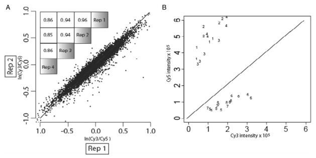
Since mRNA for each labeling was extracted from identical conditions, the true log ratio for all genes is zero. When examining multiple replicates, the observed log ratio deviates from zero due to various sources of error, such as uncontrollable biological variation between replicates and noise in the experimental analysis. If there is no gene-specific bias, the value of this deviation will vary around zero and will not be reproducible across replicates. However, as shown in Figure 1, this is strikingly not the case. When comparing two control experiments, the correlation over all log ratio values is at least 0.85, illustrating the presence of clear gene-specific bias. Since the only difference between the numerator and denominator of the log ratio is the dye used for labeling, this gene-specific effect must be dye bias. For the most affected genes, the bias effect alone can cause the ratio to deviate by more than 2-fold. Such a deviation can easily influence determination of differential expression.
Fig. 1.
Gene-specific dye bias in oligonucleotide arrays. Gene-specific dye bias is present and highly reproducible in an oligonucleotide expression microarray system. The scatter plot of panel A details a comparison of log ratio values from two separate control experiments. The inset in the upper left quantifies all six pair-wise correlations among the four replicate control experiments. As a different perspective on the same information, panel B presents the four replicateCy3 versus Cy5 intensity values for several genes (numbers 1–8) with apparent large gene-specific dye bias.
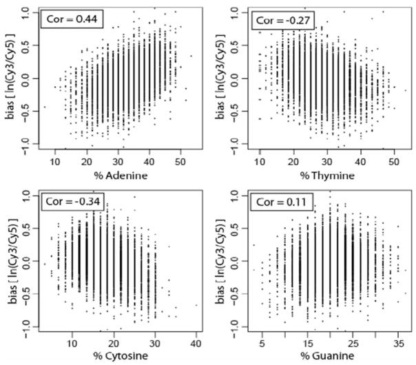
To further investigate the source of bias, we computed the correlation between the dye bias of each gene and the frequency of each nucleotide (A, C, G, T) in the sequence representing the gene on the microarray (Fig. 2). Gene-specific dye bias was measured as the average natural log ratio (Cy3/Cy5) over the four replicate control hybridizations. The most significant correlation was found with adenine content (Fig. 2A). Since the cDNA was labeled with Cy3 or Cy5 dyes conjugated to dUTP (the complement of adenine), the bias is thus proportional to the number of incorporated dye molecules. This result is then consistent with the less efficient incorporation of Cy5 dye by the polymerase.
Fig. 2.
Bias strength is related to labeled nucleotide. The upper left panel shows that strongest correlation between gene-specific dye bias in a dUTP-labeled control experiment and nucleotide content is with the frequency of adenine.
3.2 Formulating an error model
It is possible to model bias as either a multiplicative or additive error term (see Section 2). If the values of μx and μy vary substantially, the effect of an additive bias term will be different than a multiplicative one (i.e. only a multiplicative bias term will scale with the magnitude of μ). However, this distinction is irrelevant if the true intensity values for each dye (μx and μy) are equal. While this is generally not true, it is the case for the control experiments presented previously. Therefore, control data can be used to decide if it is more appropriate to model bias as a multiplicative or additive error term.
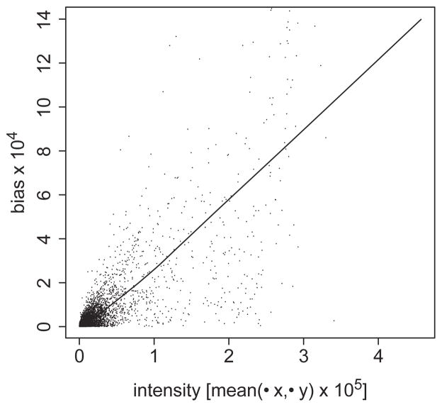
Using an additive error model, we learned bias values for each gene in the control data. Figure 3 shows the relation between the absolute magnitude of this bias and the mean signal intensity. Across different genes, there is a clear multiplicative relationship between the magnitude of bias and the mean signal intensity. An equivalent result was determined when a multiplicative error model was applied instead. Since bias terms tend to increase multiplicatively with mean intensity, it is likely more appropriate to model bias as a multiplicative error term.
Fig. 3.
Gene-specific dye bias is multiplicative in nature. The VERA error modeling procedure is applied to control data and used to determine the values of the parameters μx, μy and β for each gene. Here, the smoothed estimate of the absolute value of β is plotted as a function of the mean value of μx and μy. The data used to generate this smoothed line is also displayed as individual points.
3.3 Benchmarking model performance
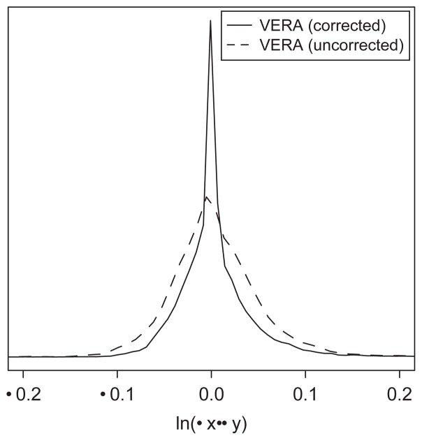
We next set out to determine whether the VERA model was able to correct for the presence of gene-specific dye bias in experimental data. The original set of control expression profiles was analyzed with both the corrected (multiplicative bias) and uncorrected (no bias) models. Figure 4 displays the distribution of ln(μx/μy) values from each analysis. In the case of the corrected VERA method, the spread of log ratio values is much tighter around the origin. Quantitatively, the variance of the uncorrected log ratios is 5.2×10⁻³, compared to 3.4×10⁻³ for the corrected algorithm. Thus, following bias correction the observed ratios tend to be closer to the true expected value of zero.
Fig. 4.
Application of dye-bias correction reduces variance in a control experiment. The solid curve represents the probability distribution of log ratio values determined following application of the corrected VERA method to control data. Conversely, application of the uncorrected VERA approach to the same data results in a distribution of log ratio values with larger variance (dashed line).
To further validate our approach and to benchmark it against other methods that have been proposed for correcting dye bias, we performed two additional sets of experiments. In each experimental set, we profiled the response of yeast to mild oxidative stress (0.1mM hydrogen peroxide versus nominal conditions) over four replicate microarrays. The only difference between sets was that in one case, dUTP was used in the labeling process, while in the other dCTP was used. Since the frequency of the labeled nucleotide within a sequence is related to its gene-specific bias (see Section 3.1), the two labeling schemes create different gene-specific dye biases while preserving the same true changes in gene expression. A method that correctly accounts for and eliminates the effect of gene-specific dye bias should maximize the agreement between these two data sets.
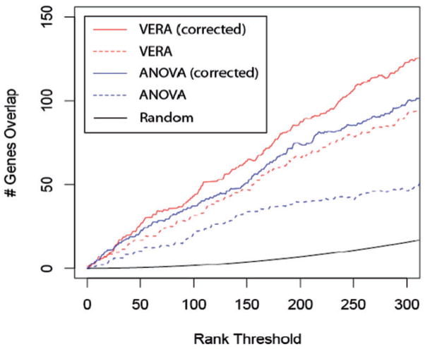
Figure 5 compares the ability of different methods to recover differentially expressed genes in the dUTP-labeled set that were identified in the dCTP-labeled set also. Previous methods to correct for GSDB model the effect as an ANOVA factor. To implement this approach, we relied upon the MAANOVA and VarMixt packages (Delmar et al., 2005; Wu, 2003). Since the true number of differentially expressed genes is unknown, this comparison was performed over a range of thresholds for calling differentially expressed genes (Irizarry et al., 2005). At nearly all possible points in this range, the bias corrected VERA approach displayed the best performance. This was followed by the corrected ANOVA statistic and the uncorrected VERA approach. ANOVA results are reported for the Fs statistic; as it previously showed the best performance over a wide range of simulated data (Cui et al., 2005). At a rank threshold of 300, the overlaps for all methods are significantly enriched over random (hypergeometric P-value=5.4×10⁻⁹ for uncorrected Fs statistic). The improvement of performance of the corrected VERA algorithm over the uncorrected one is also significant at the same rank threshold (binomial P-value=3.5×10⁻⁵). Comparison to alternative versions of the F-statistic (F1, F2, F3 and VarMixt) are available in Supplementary Figure S3.
Fig. 5.
The dCTP- versus dUTP-labeled expression data is compared for different analysis methods. Since the true number of differentially expressed genes is unknown, the calculation is performed over a range of values (x axis). The y axis shows the number of genes assumed to be significant in both labeling approaches after correcting for any bias in the method (see Section 2.7).
When the choice of labeled nucleotide is changed from dUTP to dCTP, one would expect the correlations between dye bias and nucleotide content to be altered as well. Indeed, in the dCTP labeling experiments, we observed the strongest dye bias correlation was with guanine frequency (correlation=0.39) rather than adenine frequency as observed earlier for dUTP. This reinforces the finding that the choice of labeled nucleotide has a strong impact on gene-specific dye bias.
4 DISCUSSION
The performance of VERA improved significantly when corrected for GSDB. For the ANOVA F2, Fs and VarMixt statistics, dye-bias correction also improved performance (Fig. 5 and Supplementary Fig. S3), while little to no improvement was observed for the F1 and F3 statistics. For the F1 statistic, it is likely that the lack of shared error estimates across genes in combination with the small sample size made accurate error estimation difficult, even with dye-bias correction. For the F3 statistic, the estimate of error is identical for all genes by definition. Therefore, since the dye-bias correction in the ANOVA framework affects only the relative determination of gene-specific residual error, the F3 rankings of differential expression must be identical with and without correction. VERA’s greater agreement between dCTP- and dUTP-labeled experiments (compared to ANOVA) is likely due to its more complex error model, which accounts for both additive and multiplicative errors. The ANOVA models account for multiplicative error only (which becomes additive after log transformation of the intensity values). On the other hand, ANOVA provides a flexible framework that can be easily extended to handle additional factors influencing an experiment (e.g. cell-line, treatment, dye, array).
While error models such as these can mitigate the effect of gene-specific dye bias, it would always be preferable to remove or reduce such bias if possible. Having identified nucleotide content as one contributing factor, this information might be useful in the future design of arrays. For example, probes might be chosen so as to minimize variation in adenine nucleotide content. An alternative might be to use a mix of labeled nucleotides during first strand cDNA synthesis.
In the exploratory phase of this work (see Section 3.1), we used the average ratio values determined from control experiments as an estimate of gene-specific dye bias. Only later (see Sections 3.2–3.3) was this bias modeled explicitly in the context of a probabilistic framework incorporating other errors. However, this raises an important question. Is an error modeling process required at all? Alternatively, one could simply estimate bias values from replicated controls and directly apply these estimates to future experimental results. One problem with this simpler approach is that not all genes are highly expressed under control conditions. The signals associated with low intensity genes would still be dominated by error, especially when these genes become highly expressed in some other (non-control) condition. In addition, Rosenzweig et al. (2004) noted that the gene-specific dye bias can be somewhat variable between experiments. Therefore, the values learned in a control experiment may be inapplicable, whereas the maximum-likelihood model is custom-fit to each experimental data set.
In a properly balanced microarray experiment, the influence of gene-specific dye bias on the production of false-positive measurements is mitigated, if not eliminated. As Dobbin et al. (2005) noted, the predominant effect is the generation of more false negatives. In addition, gene-specific effects can alter the ordering of significant genes, which many statistical methods rely upon. How important is it then to correct for gene-specific dye bias? This is a question that cannot be addressed in a universal manner. As shown by our experiments with different labeled nucleotides, the magnitude of gene-specific dye bias is apparently platform specific, and its impact depends critically on this magnitude in relation to the magnitude of the expression changes occurring in the biological system. Certainly, if the reliable identification of subtle differential expression changes is desired, then correcting for this systematic bias is crucial.
In summary, we have presented a method for correcting gene-specific dye bias with a maximum-likelihood model and test for differential expression. This method can effectively learn the parameters of the systematic bias without the need for additional control microarray experiments. An implementation of this algorithm is freely available at http://cellcircuits.org/VERA/.
Supplementary Material
Acknowledgments
We thank Dr. John Quackenbush for motivating discussions. We gratefully acknowledge the NSF (0425926) and NIH (GM070743) for funding this work. T.I. is a fellow of the David and Lucille Packard Foundation.
Footnotes
Supplementary information: Supplementary data are available at Bioinformatics online.
Conflict of Interest: none declared.
References
- Bolstad BM, et al. A comparison of normalization methods for high density oligonucleotide array data based on variance and bias. Bioinformatics. 2003;19:185–193. doi: 10.1093/bioinformatics/19.2.185. [DOI] [PubMed] [Google Scholar]
- Cui X, et al. Improved statistical tests for differential gene expression by shrinking variance components estimates. Biostatistics. 2005;6:59–75. doi: 10.1093/biostatistics/kxh018. [DOI] [PubMed] [Google Scholar]
- Delmar P, et al. VarMixt: efficient variance modelling for the differential analysis of replicated gene expression data. Bioinformatics. 2005;21:502–508. doi: 10.1093/bioinformatics/bti023. [DOI] [PubMed] [Google Scholar]
- Dobbin KK, et al. Characterizing dye bias in microarray experiments. Bioinformatics. 2005;21:2430–2437. doi: 10.1093/bioinformatics/bti378. [DOI] [PubMed] [Google Scholar]
- Dombkowski AA, et al. Gene-specific dye bias in microarray reference designs. FEBS Lett. 2004;560:120–124. doi: 10.1016/S0014-5793(04)00083-3. [DOI] [PubMed] [Google Scholar]
- Hekstra D, et al. Absolute mRNA concentrations from sequence-specific calibration of oligonucleotide arrays. Nucleic Acids Res. 2003;31:1962–1968. doi: 10.1093/nar/gkg283. [DOI] [PMC free article] [PubMed] [Google Scholar]
- Huber W, et al. Variance stabilization applied to microarray data calibration and to the quantification of differential expression. Bioinformatics. 2002;18 (Suppl 1):S96–S104. doi: 10.1093/bioinformatics/18.suppl_1.s96. [DOI] [PubMed] [Google Scholar]
- Ideker T, et al. Testing for differentially-expressed genes by maximum-likelihood analysis of microarray data. J Comput Biol. 2000;7:805–817. doi: 10.1089/10665270050514945. [DOI] [PubMed] [Google Scholar]
- Irizarry RA, et al. Multiple-laboratory comparison of microarray platforms. Nat Methods. 2005;2:345–350. doi: 10.1038/nmeth756. [DOI] [PubMed] [Google Scholar]
- Martin-Magniette ML, et al. Evaluation of the gene-specific dye bias in cDNA microarray experiments. Bioinformatics. 2005;21:1995–2000. doi: 10.1093/bioinformatics/bti302. [DOI] [PubMed] [Google Scholar]
- Naef F, Magnasco MO. Solving the riddle of the bright mismatches: labeling and effective binding in oligonucleotide arrays. Phys Rev E Stat Nonlin Soft Matter Phys. 2003;68:011906. doi: 10.1103/PhysRevE.68.011906. [DOI] [PubMed] [Google Scholar]
- Press, W.H. Numerical Recipes Software (Firm) Numerical Recipes in C. Cambridge University Press; Cambridge, England; New York: 1997. [Google Scholar]
- Quackenbush J. Microarray data normalization and transformation. Nat Genet. 2002;32 (Suppl):496–501. doi: 10.1038/ng1032. [DOI] [PubMed] [Google Scholar]
- Rocke DM, Durbin B. A model for measurement error for gene expression arrays. J Comput Biol. 2001;8:557–569. doi: 10.1089/106652701753307485. [DOI] [PubMed] [Google Scholar]
- Rosenzweig BA, et al. Dye bias correction in dual-labeled cDNA microarray gene expression measurements. Environ Health Perspect. 2004;112:480–487. doi: 10.1289/ehp.6694. [DOI] [PMC free article] [PubMed] [Google Scholar]
- Tseng GC, et al. Issues in cDNA microarray analysis: quality filtering, channel normalization, models of variations and assessment of gene effects. Nucleic Acids Res. 2001;29:2549–2557. doi: 10.1093/nar/29.12.2549. [DOI] [PMC free article] [PubMed] [Google Scholar]
- Wu H, et al. MAANOVA: a software package for the analysis of spotted cDNA microarray experiments. In: Parmigiani G, et al., editors. The Analysis of Gene Expression Data: An Overview of Methods and Software. Springer; New York: 2003. pp. 313–431. [Google Scholar]
- Yang YH, et al. Normalization for cDNA microarray data: a robust composite method addressing single and multiple slide systematic variation. Nucleic Acids Res. 2002;30:e15. doi: 10.1093/nar/30.4.e15. [DOI] [PMC free article] [PubMed] [Google Scholar]
- Young RA. Biomedical discovery with DNA arrays. Cell. 2000;102:9–15. doi: 10.1016/s0092-8674(00)00005-2. [DOI] [PubMed] [Google Scholar]
Associated Data
This section collects any data citations, data availability statements, or supplementary materials included in this article.


