

Abstract
We apply modeling approaches to investigate the distribution of late recombination nodules in maize (Zea mays). Such nodules indicate crossover positions along the synaptonemal complex. High-quality nodule data were analyzed using two different interference models: the “statistical” gamma model and the “mechanical” beam film model. For each chromosome, we exclude at a 98% significance level the hypothesis that a single pathway underlies the formation of all crossovers, pointing to the coexistence of two types of crossing-over in maize, as was previously demonstrated in other organisms. We estimate the proportion of crossovers coming from the noninterfering pathway to range from 6 to 23% depending on the chromosome, with a cell average of ∼15%. The mean number of noninterfering crossovers per chromosome is significantly correlated with the length of the synaptonemal complex. We also quantify the intensity of interference. Finally, we develop inference tools that allow one to tackle, without much loss of power, complex crossover interference models such as the beam film. The lack of a likelihood function in such models had prevented their use for parameter estimation. This advance will allow more realistic mechanisms of crossover formation to be modeled in the future.
INTRODUCTION
Meiosis allows the segregation of homologous chromosomes (homologs) in sexually reproducing organisms to produce haploid gametes from parental diploid cells. During prophase I of meiosis, DNA double-strand breaks are initiated by the Spo11 topoisomerase-like transesterase (Keeney et al., 1997) and repaired using a homologous nonsister chromatid as a template. This leads to either reciprocal exchanges (crossovers [COs]) affecting the rest of the chromosome arm or nonexchange events (noncrossovers [NCOs]), which may be detected through associated gene conversions localized to small segments (Bishop and Zickler, 2004). Crossovers have two major consequences: (1) they create physical connections (visible as chiasmata) that, in association with sister chromatid cohesion, hold the homologs together in stable pairs (bivalents) ensuring proper segregation at anaphase I (Page and Hawley, 2003; Jones and Franklin, 2006), and (2) they induce reciprocal exchanges of large fragments of genetic material, leading to intrachromosomal reshuffling of parental alleles in the gametes. CO frequencies define the genetic distance unit (centimorgan [cM]), so a 100-cM (= 1 morgan) segment experiences on average 1.0 CO per gamete (which is equivalent to an average of two COs among the four chromatids of each bivalent). The number of COs per chromosome is highly regulated: typically at least one chiasma occurs per bivalent (referred to as the obligate CO) in most organisms (Jones, 1984; Jones and Franklin, 2006), and the size range of genetic linkage maps is much more constrained than physical genome sizes across different species.
The distribution of COs along chromosomes is clearly nonrandom. Some regions of the physical chromosome are much more prone to CO formation and recombination than others, and some regions (for example, near centromeres) hardly ever recombine (Jones, 1984; Anderson and Stack, 2002; Drouaud et al., 2006). In addition, a phenomenon called CO interference (Sturtevant, 1915; Muller, 1916) lowers the probability that two COs occur close to each other in the same meiosis. Interference has been reported in most organisms tested, with some exceptions, such as Schizosaccharomyces pombe and Aspergillus nidulans (Zickler and Kleckner, 1999). Experimental results from several organisms indicate that even though most of their meiotic COs are subject to interference, a small fraction of COs shows little or no interference. These organisms include yeast (Saccharomyces cerevisiae; Hollingsworth and Brill, 2004; Stahl et al., 2004), tomato (Solanum lycopersicum; Lhuissier et al., 2007), Arabidopsis thaliana (Higgins et al., 2004; Mercier et al., 2005), and mouse (Mus musculus; Guillon et al., 2005). The interfering pathway (hereafter referred to as Pathway 1 or P1) depends on genes from the ZMM family as well as Mlh1 and Mlh3, while the noninterfering (or weakly interfering) pathway (Pathway 2 or P2) partially depends on Mus81 and associated proteins (Hollingsworth and Brill, 2004; Mézard et al., 2007). From these studies, the proportion of P2 COs seems to be variable across species with values from 0 to 23% in mouse (Froenicke et al. 2002; Broman et al. 2002; Falque et al. 2007) up to ∼30% in yeast (de los Santos et al. 2003; Hollingsworth and Brill 2004) and tomato (Lhuissier et al., 2007). At the two extremes are Caenorhabditis elegans that has only interfering COs and S. pombe that has only noninterfering COs.
CO positions may be experimentally determined by studying recombination between genetic markers in high-density linkage mapping experiments or by direct cytological observations. In the latter case, one can measure CO positions by visualizing late recombination nodules using electron microscopy (Sherman and Stack, 1995; Anderson et al., 2003) or by immunofluorescence using antibodies against different proteins that concentrate as foci at the location of COs (Lawrie et al., 1995; Froenicke et al., 2002; de Boer et al., 2006). Interestingly, P1 (interfering) COs can be specifically detected using immunolocalization of MLH1, one of the proteins involved in this pathway of CO formation. By contrast, late recombination nodules (LNs) in tomato and maize (Zea mays) are thought to mark all COs from both P1 and P2 pathways (Sherman and Stack, 1995; Anderson et al., 2003; Lhuissier et al., 2007). Lhuissier et al. (2007) demonstrated that ∼70% of the LNs in tomato were immunolabeled with MLH1, indicating that P1 accounts for the majority of COs in tomato, with the remaining 30% of COs thought to be associated with the P2 pathway.
To analyze statistical features of CO formation, some empirical indicators, such as the coefficient of coincidence (Ott, 1999), may be used, but the most powerful approach is to fit mathematical models to experimental data sets. The multiple models proposed so far are based on very different approaches to generate interference between COs, and they may be roughly grouped into two classes: physically motivated models and statistically oriented models. Physical models include one that simulates the polymerization along the chromosome axis of a complex that initiates at CO locations and inhibits nearby CO formation (King and Mortimer, 1990). Another physical model called “beam film model,” hereafter referred to as BF model, simulates establishment and propagation of a mechanical stress along the lateral element with COs being seen as cracks that release the stress locally and thus forbid nearby COs (Kleckner et al., 2004). Statistical models, on the other hand, are mainly based on the statistics of genetic distances between successive COs. These models use stationary renewal processes (SRPs; McPeek and Speed, 1995; Zhao and Speed, 1996) that draw useful mathematical properties from the hypothesis that inter-CO distances are independent and identically distributed. Among SRP-based models, one of the most studied is the gamma model (McPeek and Speed, 1995), and we shall use it in this work. The model's name comes from the fact that inter-CO distances follow a gamma distribution. Interestingly, when the interference parameter of the gamma model takes integer values, the model is equivalent to the counting or χ2 model (Foss et al., 1993). In the counting model, two adjacent COs are separated by a given number of NCOs, leading to a fixed CO/NCO ratio. This framework allows for a mechanistic interpretation of interference (Stahl et al., 2004). Note that in some cases, the CO/NCO ratio varies between the wild type and mutants (Martini et al., 2006), while in other cases, the CO/NCO ratio is stable (Mehrotra and McKim, 2006; Stahl and Foss, 2009). Finally, the Forced Initial Crossover model (Falque et al., 2007) is a variant of the counting model that takes into account the biological constraint of the obligate CO.
SRP-based models have been the preferred approach for analyzing biological data sets because other models often involve too many parameters and/or lack convenient inference methods to fit data (e.g., maximum likelihood fitting). Moreover, little is known about the biological basis of real interference mechanisms (Zickler and Kleckner, 1999) so physical models have little substance upon which to draw and have been kept out of favor so far. By contrast, given the simplicity of the SRP-based models, these have been extensively used to study CO position data sets available for different organisms.
Incorporating two pathways (P1 and P2) of CO formation in models is most simply achieved by sprinkling P2 COs over P1 COs. That is, P1 CO positions are generated using an interference model first, and then P2 CO positions that are generated through a Poisson model without interference are superimposed on the P1 distribution (Copenhaver et al., 2002). Such two-pathway models assume that P1 and P2 COs are produced through independent processes. Using the gamma model for P1 and adding P2 sprinkling has led to inferences of the proportion of P2 COs ranging within 19 to 20% for Arabidopsis chromosomes 1, 3, and 5 (Copenhaver et al., 2002), 3 to 5% for Arabidopsis chromosomes 2 and 4 (Lam et al., 2005), 0 to 21% (and mostly <10%) in humans (Housworth and Stahl, 2003), and around 10% for yeast chromosome 7 (Malkova et al., 2004).
Here, we analyze LN positions in maize (Anderson et al., 2003). LNs are thought to mark all CO positions (Anderson and Stack, 2002; Anderson et al., 2003; Lhuissier et al., 2007), so we shall simply refer to LNs as COs in the rest of this work. We include in our modeling of interference both the gamma model (McPeek and Speed, 1995), based on a statistical approach, and the BF model (Kleckner et al., 2004), based on a physical approach. This latter model has not been used for data analysis before because of the numerous technical difficulties involved. Thanks to the inference tools we developed, namely, to exploit the BF model, we unravel here the contributions of each pathway and their properties for each of the 10 chromosomes of maize. In particular, we exhibit the presence of two CO formation pathways.
RESULTS
Correspondence between Single-Pathway Interference Models
The frameworks assumed for the gamma and the BF models are very different. Nevertheless, they both incorporate interference, which leads to a rarefaction of nearby COs. It is thus conceptually useful to introduce a correspondence between the two models via the strength of the interference they produce. There is no unique measure of this strength, but a convenient indicator of interference strength is simply the relative width of the distribution of CO interval lengths. Explicitly, for any given model, let ρ (Δ) be the probability density of CO interval lengths Δ (where Δ is the distance between two successive COs). For definiteness, assume that this distribution is obtained for a chromosome of given genetic length. Our indicator of interference strength is then the coefficient of variation CV = σ(Δ)/μ(Δ), where μ and σ are the mean and sd of the distribution of Δ. For instance, with an infinite chromosome, the gamma model, whose interference parameter is ν, leads to 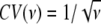 . As interference becomes strong, CV goes to zero and COs become regularly spaced. In the BF model, whose interference parameter is λ, CV(λ) has to be determined by simulation, which can be done to whatever accuracy is needed.
Given the two functions CV(ν) and CV(λ), we brought a value of ν in correspondence with that value of λ, which gave the same CV. This results in a map between ν and λ (see Supplemental Figure 1 online for two choices of chromosome lengths, those of chromosomes 1 and 10 in maize). The most distinctive feature we see in this figure is that the BF model does not produce interference strengths beyond a maximum value that depends on chromosome size. In particular, CV in the BF model goes to a limiting (strictly positive) value when λ becomes arbitrarily large. For example, for the size of maize chromosome 1, CV tends to 0.27 as λ goes to infinity, corresponding to the maximum value ν = 13.2 (see Supplemental Figure 1 online). By contrast, in the gamma model, as ν grows, CV goes to 0. What is the source of this difference? The BF model has precursors that are distributed at random and thus can never generate perfectly regular interval lengths. Going from the precursors to the COs in that model introduces some regularity in the CO positions, but the fluctuation in Δ is always comparable to the distance between two precursors, so very strong interference is simply not possible in the BF model as it stands.
Presence of Two Distinct Types of COs
The two models were fitted to the experimental data giving the LN positions for ∼200 meioses (see Methods). For each of the 10 chromosomes, we estimated the proportion p of pathway 2 (P2) COs when using either the gamma model or the beam film model for pathway 1 (P1), while P2 is applied by sprinkling noninterfering COs on top of those coming from P1. Hereafter, we refer to these two cases as the GS and BFS models, respectively. Results are given in Figure 1 for GS (see Supplemental Figure 2 online for BFS). We also determined the associated confidence intervals of this parameter p as explained in Methods. Data for each chromosome were incompatible at the 98% significance level with the value p = 0 for both the GS and the BFS models. Combining these intervals for all chromosomes, the cell-wide single pathway case was excluded far beyond the 99.9% level. The values estimated for p fell between 6 and 23% depending on the chromosome and on the model. At a whole-cell level, the total contribution of P2 was estimated at 13% with the GS model and 18% with the BFS model.
Figure 1.

Interference Intensity and Proportion of Noninterfering COs Using the GS Model.
Estimated values of the interference intensity (ν) in the pathway P1 and proportion of pathway P2 COs (p), obtained by maximum likelihood fitting the GS model to maize LN data for each chromosome. Horizontal and vertical bars indicate 95% confidence intervals based on 1000 simulated data sets. For chromosome 8, the upper bound of the CI on ν is 14.1.
To see whether our two models lead to compatible estimates for p, we compared the corresponding pairs of inferred values (see Supplemental Figure 3 online). In case of compatible estimates, each point should be close to the x = y line. More quantitatively, for each point, the rectangle built from the x and y confidence intervals should cross that line. We see that this is the case for nearly all chromosomes (chromosome 3 is the only exception), but we also see that the estimates in the BFS model are systematically higher than those in the GS model.
Interference Strength Varies Little from Chromosome to Chromosome
For each of the 10 chromosomes, we estimated the interference strength of pathway 1 (ν for the GS model and λ for the BFS model) as well as its associated 95% confidence intervals. In the GS model (Figure 1), we found 4.2 < ν < 6.2 for the estimated values, except for the outlier chromosome 8 for which ν = 9.6. Removing that chromosome, all others were compatible with ν = 5, suggesting that interference varies little from chromosome to chromosome. However, including chromosome 8, we rejected the hypothesis of a common value of ν for all chromosomes using the χ2 test (P value = 0.016). Note that going from ν = 4.2 to ν = 6.2 corresponds to reducing the inter-CO standard deviation merely by 18%.
In the BFS model (see Supplemental Figure 2 online), we found 0.08 < λ < 0.16 except for the outlier chromosome 2. That chromosome seems to have an interference strength higher than can be parameterized in the BF model; thus, formally λ is infinite there.
Little Power Is Lost with the PLS Fitting Score
It is appropriate to consider the dependence of the inferred parameters on the fitting procedure. In the case of the GS model, the fits shown in Figure 1 were performed using the maximum likelihood method. For the BFS (see Supplemental Figure 2 online), the likelihood of a bivalent cannot be computed because the CO positions in that model result from a complicated process. We thus had to resort to fitting using a goodness-of-fit approach based on the PLS score function of Equation 1 (see Methods). Consider now whether the two fitting methods (likelihood and PLS score) give compatible estimates in practice. We compared the inferred parameters p and ν in the GS model of Figure 1 to what was found for the same GS model when using the PLS score (see Supplemental Figure 4 online). For the same data and model, the two fitting methods gave rise to very similar and compatible values. Furthermore, we see that the confidence intervals of the fits based on PLS were just a bit larger than those based on maximum likelihood. It is then fair to say that by replacing the true likelihood by the PLS score, little accuracy and power was lost. To make this statement more quantitative, we have computed by simulation the confidence intervals for both of these methods as a function of the number of bivalents in the data set, using simulated data (see Supplemental Figure 5 online). When increasing the number N of bivalents, the bias (as measured by the difference between the median simulated value and the true value) decreased with a law compatible with 1/N, and similarly, the size of the confidence interval decreased with a law compatible with  . For these simulations, we used the resimulation method described in Methods applied to chromosome 1.
Agreement between Models and Experimental Data
We saw that the fits gave confidence intervals that excluded p = 0 for both the GS and the BFS models. One thus suspects that the single-pathway models must lead to poor adjustments to some features of the experimental data, and so it is natural to ask what in fact these features are. Not surprisingly, we found that the p = 0 models provided good adjustments to the frequencies P(0), P(1), P(2). . . of bivalents with 0, 1, 2. . . COs, confirming the claim that these frequencies are not very discriminative of different models (Broman and Weber, 2000). More likely, the single-pathway models should have difficulty reproducing the shape of the inter-CO distances (Δ). The reason is that if sprinkling is present at a low level, most inter-CO distances will be due to two COs from P1 for which essentially no small values of Δ can occur. Nevertheless, a small fraction (proportional to p) of such distances will arise due to one CO from P1 and one from P2. Having no sprinkling (i.e., using a single-pathway interfering model) excludes a non-zero density of inter-CO distances Δ as Δ approaches zero. In Figure 2, we show the distribution of Δ as obtained from the experimental data (bars) and from the adjusted models (lines) for chromosomes 1 and 10. The analogous data for all chromosomes is provided in the supplemental data (see Supplemental Figures 6 and 7 online). Clearly, the adjustments for the single-pathway models (gamma or BF with p = 0) are much less good than for the two-pathway models (GS and BFS). This is quantified by the sum of squares of the differences between experimental and adjusted model values as reported in the figures. We also find that these sums of squares have lower values for GS than for BFS, suggesting that the gamma-based model gives better adjustments to the data. For completeness, the No-Interference model, which corresponds to p = 0 and ν = 1, is also represented in these figures. Finally, as expected, we see that the single-pathway models that include interference tend to give curves that rise too fast near Δ = 0 to compensate for the fact that such models predict extremely few COs very close to each other. The same conclusions hold for the other chromosomes (see Supplemental Figures 6 and 7 online).
Figure 2.

Quality of the Fits Obtained with Single-Pathway or Two-Pathway Models.
Density distribution of distances between adjacent LNs in all SCs with at least two LNs for maize chromosomes 1 and 10. The x axis shows the relative genetic distance. Bars indicate experimental observations. Lines indicate simulations with no interference (NI), single-pathway gamma model (G), two-pathway gamma-sprinkling model (GS), single-pathway BF model (BF), or two-pathway BFS model (BFS). The sum of squares of differences between experimental and simulated densities are in parentheses.
Correlations with Chromosome Length
How are p and interference strength correlated with the length of the synaptonemal complex (SC)? The parameter ν in the GS model had no significant correlation with SC length measured in micrometers (see Supplemental Figure 8 online, left panel). The same conclusion held for the BFS model. In the previous section, we saw that the GS model systematically gave better fits than the BFS, so we focus here on the GS results. Considering now the values of p as a function of SC length (see Supplemental Figure 8 online, right panel), there seems to be an association between the two values, but it is not statistically significant (the P value associated with the hypothesis of no association is 0.125). We found two outliers (chromosomes 3 and 8), which might shed some doubt on the relevance of such an association. We also found that the data looked very similar when using the genetic length instead of the SC length. The reason for this is simply that these two lengths are very strongly tied as was previously shown (Anderson et al., 2003). It seems possible that genetic and SC lengths are smoothly related and that any visible deviations are simply due to sampling effects (see Supplemental Figure 9 online). Considering now the numbers of P1 and P2 COs per chromosome, in both cases there was a significant correlation with SC length (see Supplemental Figure 10 online).
DISCUSSION
The presence of two pathways for meiotic CO formation, one with interference (P1) and the other with little or no interference (P2), is found among such diverse organisms as budding yeast, mammals, and plants (de los Santos et al., 2003; Hollingsworth and Brill, 2004; Mézard et al., 2007). Among plants, the supporting data comes from two dicots, Arabidopsis and tomato. In Arabidopsis, mathematical modeling of CO distribution in tetrads from wild-type plants as well as analysis of mutants reveal the presence of the two pathways (Copenhaver et al., 2002; Higgins et al., 2004, 2008a; Mercier et al., 2005; Berchowitz et al., 2007). In tomato, cytological MLH1 immunolabeling of a subset of LNs in pachytene SC spreads similarly supports the presence of two pathways of crossing-over (Lhuissier et al., 2007). Monocots would be expected to have and use these two pathways of crossing-over also, but no studies have examined this question, largely because of a lack of appropriate tools to do so. Here, for maize, using the gamma and BF models for crossing-over, we examined the behavior of each pathway and inferred their contributions by comparing to LN data (Anderson et al., 2003). The high quality of the LN data set allowed us to exhibit the presence of two different classes of COs in a monocot and to unravel the separate features of each class for each of the 10 chromosomes of maize. In addition, we developed an innovative method using the PLS score, by which one can fit any complex model to experimental data even if no likelihood function can be derived; this was crucial for using the BF model.
To our knowledge, this is the first time that LNs have been used to explore these different models for CO pathways, and the approach is based on evidence that LNs faithfully mark the locations of COs (Zickler and Kleckner, 1999; Anderson and Stack, 2002; Lhuissier et al., 2007). For example, the number and distribution of LNs mirrors that of chiasmata in maize (Anderson et al., 2003). It should be noted that the corresponding mean number of COs deduced in maize is nevertheless smaller than when using molecular linkage maps (Davis et al., 1999). Such discrepancies between cytological and genetic maps have been noted for several different organisms, and a large part of the difference can be attributed to factors such as mapping errors that lead to inflation of linkage maps (Anderson and Stack, 2002; King et al., 2002; Lynn et al., 2004). We cannot exclude the possibility that some LNs were missed during construction of the LN map in maize, although given the close correspondence between LNs and chiasmata, this must not be a common occurrence. This putative loss would mainly affect close-by COs, which would underestimate the contribution of pathway 2 rather than introduce an artifactual noninterfering pathway.
Proportion of COs Attributable to a Noninterfering Pathway in Maize
The results show that our models based on a single interfering pathway for crossing-over are inadequate to describe the observed distribution of LNs in maize. We found that p = 0 (i.e., no P2 COs) is excluded for each chromosome at the 98% confidence level. Note that this conclusion holds in two very different kinds of models, and probably the most important cause for the inadequacy of these single-pathways models is that they cannot produce close-by COs. In essence, this means that two types of COs must coexist in maize, with one type allowing for small inter-CO intervals. If, as is generally accepted, interference in P1 forbids such small intervals, then there must be a second pathway in maize.
Going from one- to two-pathway models leads to much better fits to the observed LN distribution data, as seen in Figure 2. For both our two-pathway models, the inferred values of p range from 6 to 23%. However, they are not far from being compatible with a single value given the confidence intervals. Within the gamma model, that fits closest to the data, all chromosomes except for 1 and 10 are compatible with the value p ∼12%. However, chromosomes 1 and 10, the largest and smallest chromosomes, respectively, almost surely have distinct values for p as their confidence intervals do not overlap; this conclusion holds in both models (Figure 1; see Supplemental Figure 2 online).
How do these values compare with estimates of p for other species? Three different approaches have been taken to estimate the contribution of P2 to total CO number in different organisms.
One approach is to fit CO data to the gamma with sprinkling (GS) model, as is done in this work. Malkova et al. (2004) estimated p to be between 8 and 12% for budding yeast chromosome 7. Copenhaver et al. (2002) inferred p for each of the five chromosomes of Arabidopsis using data sets of ∼60 bivalents (from tetrads) and obtained values ranging from 0 to 20%. Using data sets of ∼90 gametes (not bivalents), Housworth and Stahl (2003) inferred values ranging from 0 to 21% for different chromosomes in humans. Thus, the maize value (based on 2080 SCs) of p ∼12% is within the ranges reported for these organisms.
A second approach is to compare total map length (based on LNs or genetic data) with the mean number of MLH1 foci on bivalents. MLH1 foci are thought to label specifically the positions of COs from P1 and thus allow one to extract (1-p) LG, where LG is the genetic length of the chromosome. Using this approach, p was found to be ∼30% for tomato (Lhuissier et al., 2007). For mouse chromosomes, using published data from Froenicke et al. (2002) and Broman et al. (2002), p can be estimated at 0 to 23%, depending on the chromosome.
Finally, a third approach to estimate p is through analysis of mutants that are thought to knock out one of the two CO pathways. Naturally in such mutants, homeostasis effects may arise, so there is no guarantee that the remaining COs provide reliable values of p. Nevertheless, here again the range of values of p is not substantially different from those found using the other methods. For instance, in mouse, using mlh1−/− (Guillon et al., 2005) and mlh3−/− (Holloway et al., 2008) mutants, the P2 pathway was estimated to account for 5 to 10% of all COs. This is to be compared with a proportion of 11% in the wild-type mouse as deduced from MLH1 data of Froenicke et al. (2002) and genetic data of Broman et al. (2002). In Arabidopsis, several works based on mutants lead to estimating p between 10 and 20%. For instance, the number of chiasmata is reduced to 15% of the wild-type level in msh4 mutants (Higgins et al., 2004), to 11 to 18% in zip4 mutants (Chelysheva et al., 2007), to 11 to 14% in shoc1 mutants (Macaisne et al., 2008), and to 13% in msh5 mutants (Higgins et al., 2008b). On the other hand, 9 to 12% reductions of recombination rate were observed in mus81 mutants using large tetrad data sets (Berchowitz et al., 2007), although no significant reduction of chiasmata counts could be detected by Higgins et al. (2008a). Interestingly, all these results are compatible with the value p = 14% that comes from the modeling estimates of Copenhaver et al. (2002) using wild-type plants.
Strength of Interference in P1
The interference strength parameter (ν) estimated for P1 in our study with the GS model is close to ν = 6 for all chromosomes (Figure 1), except chromosome 8, which gives a significantly higher interference strength (ν = 11). There seems to be no association between ν and SC length (see Supplemental Figure 8 online).
With the BFS model, interference strength is parameterized by λ, which is proportional to the characteristic distance over which stress can propagate. We found λ values compatible with λ = 0.1 for six of the 10 maize chromosomes (see Supplemental Figure 2 online). However, λ estimates for chromosomes 7, 8, and 9 were larger (λ > 0.13). Furthermore, for chromosome 2, λ is infinite; as we demonstrated (see Supplemental Figure 1 online), the BF model has an intrinsic limitation on interference strength, which is responsible for this result.
The other main outliers are chromosomes 7 and 8. Compared with the other chromosomes, their histograms (see Supplemental Figures 6 and 7 online) have bimodal shapes. Clearly, the models have difficulty reproducing the somewhat irregular structure of the experimental histograms for these chromosomes. In particular, both experimental histograms have the bin at 0.55 with an anomalously large value, pushing the fitted interference strength to be high.
Other authors have estimated interference strength in P1 by fitting inter-CO distances to a gamma distribution. However, as shown by Housworth and Stahl (2009), this is not equivalent to using the gamma model because there are finite chromosome size effects. If chromosome size is not considered properly when applying the gamma model, artifactual interchromosome trends can result. Values of ν have been estimated for Arabidopsis to be between 10 and 21 (Copenhaver et al., 2002). In humans, a first study estimated ν to be between 2.2 and 10 for most chromosomes (Housworth and Stahl, 2003). More recently, the same authors (Housworth and Stahl, 2009) have shown that CO data from human males are consistent with constant interference levels among chromosomes of all sizes.
Another method to estimate interference strength in P1 is to use single-pathway models on data sets reflecting the positions of P1 COs only, such as MLH1 foci mapping along SCs. This approach gave ν = 7.9 and ν = 6.9 for tomato chromosomes 1 and 2 (Lhuissier et al., 2007). In mouse, MLH1 foci data from Froenicke et al. (2002) gave interference strengths corresponding to ν between 5 and infinity (Falque et al., 2007). Using the gamma model on other mouse MLH1 data, de Boer et al. (2007) estimated ν = 7.5 and ν = 10.1 for chromosomes 1 and 2, and Barchi et al. (2008) estimated ν values from 12 to 25. Estimates of ν were also obtained in dog (6.5; Basheva et al., 2008), cat (3.7; Borodin et al., 2007), and shrew (11 to 16; Borodin et al., 2008). Thus, the ν values of 4.5 to 11.5 that we obtained for maize are within the range of those observed for other plants and for mammals. Finally, there have been estimates of ν using the counting or gamma model (single-pathway) on data that include both P1 and P2 COs, although this approach obviously introduces a bias in the inferred values. Not surprisingly, such an approach underestimates the interference strength as clearly shown by Copenhaver et al. (2002). In support of this, mutants that lack P2 COs show enhanced interference effects (Berchowitz et al., 2007).
Comparison between the Gamma and Beam Film Models
Analyses of CO patterns have largely used the gamma model to infer the level of CO interference (see previous section). Probably the main reason for this choice is that the gamma model allows for a tractable formula for the likelihood of any meiotic product. Another choice for modeling CO interference is the BF model (Kleckner et al., 2004), which postulates a mechanism responsible for interference. However, the model lacks a computable likelihood function, which makes it difficult to apply to data sets. To overcome this technical difficulty, we have introduced an approach using a score (PLS) to quantify the goodness of fit between the BFS model's predictions and experimental data. Interestingly, very little inference power is lost in the GS model when using the PLS score instead of the likelihood (see Supplemental Figure 5 online). With this inference tool, either model can be used for fitting data, even though the two models have little in common.
We used the coefficient of variation of inter-CO distances to map one model onto the other. This mapping (see Supplemental Figure 1 online) revealed that, in contrast with the gamma model, the BF model does not allow inter-CO distances to be too narrowly distributed. In effect, the BF model has a maximum interference strength when it is mapped onto the gamma model, and we find this maximum to be generally higher for shorter chromosomes (see Supplemental Figure 1 online). Maize chromosome 2 seems to be very close to this maximum interference strength reachable by the BF model. When performing fits on this chromosome, we were led to very large values for λ and huge confidence intervals (see Supplemental Figure 2 online). In this situation, the BFS may not allow us to infer a finite value of λ, which is a weakness of the model.
Although the results for interference strength using statistical and physical models are only approximately comparable, an unambiguous comparison of the proportion of COs due to P2 (p) using the GS and the BFS models is possible since the meaning of p is defined outside of any model. We find that the BFS model gives rise to slightly larger estimates of p than the GS model (see Supplemental Figure 3 online). Generally speaking, when a parameter has significantly different estimates using two different methods, the values inferred should be considered with caution. In this precise case, we also found that the goodness of fit provided by the GS model was systematically better than that provided by the BFS (see Supplemental Figures 6 and 7 online). Thus, it seems justified to give greater credence to the estimates of p coming from the GS model, and for the rest of the discussion, we will focus on the gamma model only.
Correlations between SC Length and Individual Pathway Contributions
Several studies in different organisms have shown that genetic length (LG) is positively correlated with SC length (LSC); presumably this correlation arises from a coordinated regulation, although the possible mechanisms are still unknown (reviewed in Kleckner et al., 2003). At a more quantitative level, Housworth and Stahl (2003, 2009) proposed that a general formula relating genetic length to physical length LP, such as LG = a LP + b might hold qualitatively for all the chromosomes in a given organism. In their framework, the term “a LP” is the mean number of COs coming from pathway P1. Similarly, “b” is the mean number of COs coming from pathway P2. Since in this formula, “b” is chromosome independent, all chromosomes have the same mean number of P2 COs. Furthermore, taking “A” to be the density of precursors on the chromosome per base pair, Housworth and Stahl (2003) obtain for the gamma model the relation a = A/ν; since “a” is taken to be chromosome independent, this means that all chromosomes are subject to the same intensity of interference.
Most organisms have strongly correlated LP and LSC (Anderson et al., 1985). Thus, the formula of Housworth and Stahl motivates testing a similar linear relation between LG and LSC, namely, LG = a LSC + b. This formula is in good agreement with our data (see Supplemental Figure 9 online). The regression also shows that there is clearly a very significant association between these two lengths. Extrapolating this regression line to LSC = 0, we obtained the intercept LG = 32.4 cM. However, for very short chromosomes, one expects LG = 50 cM according to the obligate CO rule. This means that the linear relation LG = a LSC + b has to be corrected for small SC sizes, unless the obligate CO rule suffers some exceptions in maize.
Consider now the parameters “a” and “b” successively. As shown in Figure 1, all chromosomes, except for number 8, are compatible with a constant interference strength (ν = 5). In analogy with the framework used by Housworth and Stahl, this would be expected if the parameter “a” was constant. To give further credence to this hypothesis, we show that there is no trend between ν and LSC (see Supplemental Figure 8 online, left panel). A similar analysis was performed for the parameter “b.” We determined the mean number of P2 COs versus LSC (see Supplemental Figure 10 online, right panel). The regression line seems to exclude the hypothesis of constant “b” (P value = 0.008), although it can be noted that essentially all the correlation comes from chromosomes 1 and 10. If “b” were constant, the proportion p of P2 COs would be a decreasing function of LSC, which seems incompatible with the data (see Supplemental Figure 8 online, right panel). In view of these data, there is an alternative hypothesis to having a constant “b”: the mean number of P2 COs may be roughly proportional to LSC. While our data do not contradict this alternative hypothesis, there is much scatter in the cloud of points (see Supplemental Figure 10 online). Providing more convincing evidence would require significantly more bivalents than in this study.
To make further progress and unveil in greater detail additional properties of the two pathways, larger data sets would be useful. More generally, as the quality of experimental data improves, it will become worthwhile to conceive more realistic and complex models of CO formation. The exploitation of any such models for data fitting will be possible with the inference techniques we developed here for the BFS, whereby we overcame the problem of having no computable likelihood function. On the experimental side, new insights would be obtained if one could identify the pathway giving rise to each individual CO or its cytological counterpart (LNs, MLH1, etc.). Such data would allow direct measurements of p that could be compared with estimates coming from different models. Even more interestingly, such explicit information on P1 and P2 COs would allow one to test the hypothesis that these two pathways are independent.
METHODS
Maize (Zea mays) LN Distributions
All of the LN data used in the analyses here are from Anderson et al. (2003). Male microsporocytes from the inbred maize line KYS were used for preparing the LN distributions from spreads of SCs (see picture in Figure 3). Individual SCs were identified from sets of spread SCs, based on relative length and arm ratio. The positions of 4267 LNs on a total of 2080 SCs were mapped by electron microscopy. The plants were maintained in a temperature-controlled greenhouse to minimize environmental variation.
Figure 3.

Electron Micrograph Showing Late Nodules on SCs.
Electron micrograph of a portion of a spread of SCs from maize primary microsporocytes in pachytene showing bivalents 4, 8, and part of 5 (left) and higher magnification views (right) of SC segments with RNs (labeled with arrowheads and the same lowercase letters at the two magnifications). Each SC has been identified based on its relative length and arm ratio, and in this set, the kinetochores (K) of bivalents 4 and 8 are fused together. A halo of dispersed chromatin is visible around each SC. Bar = 5 μm (left). Magnification for the right column is 2.5 times higher.
Interference Models
For modeling interference in the P1 pathway, we use the gamma model (McPeek and Speed, 1995), which is the most frequently used SRP-based statistical model, and the BF model (Kleckner et al., 2004), which is a very mechanistic physical model. To include a second pathway, we use the sprinkling procedure (Copenhaver et al., 2002) whereby noninterfering P2 COs are simply added to those of P1.
Estimation of Parameters and Confidence Intervals
Our goal is to determine the proportion of P2 COs and the interference strength of P1 in maize. We estimate these values by searching for the parameters of our models that give the best fit to the experimental data. For the gamma and GS models, we do this by maximizing the likelihood of the data set as a function of these parameters. The formulas for the likelihoods have been previously published by Broman and Weber (2000) for the gamma model and by Copenhaver et al. (2002) for the GS model. Unfortunately, for complex models such as the BF, it is not possible to compute the likelihood of having a given list of CO positions on a bivalent. We have thus developed a scoring method to measure the goodness of fit as follows. Let P(0), P(1), P(2), . . . be the probability in the model of obtaining 0, 1, 2, . . . COs on a bivalent and let ρk be the probability density of inter-CO distances for bivalents with exactly k COs. Our projected likelihood score (PLS) is then defined by:
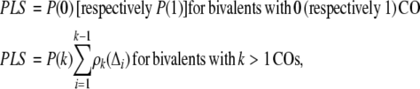 |
(1) |
where Δi is the i'th interval length (between CO i and CO i+1). Fitting the model then consists in finding the parameters p and λ that maximize the PLS. For both the likelihood (GS model) and the PLS (BFS model), we have designed an efficient hill-climbing algorithm that renders the two-dimensional search computationally feasible. An illustration of the shape of the hill to climb is given in Figure 4 for the PLS.
Figure 4.

Landscape of the PLS Score to Be Maximized for Two-Dimensional Parameter Inference.
Projected likelihood score (PLS; based on inter-CO distances; see text) as a function of the two parameters of the BFS model. λ, interference intensity in the interfering pathway; p, proportion of COs formed through the noninterfering pathway (P2).
Given the optimal parameters, we follow Viswanath and Housworth (2005) to obtain their confidence intervals. This is done by fitting 1000 simulated data sets, which provides an approximation to the distribution of each inferred parameter. Extracting the associated 95% confidence interval is then straightforward; one just has to find the tails containing 2.5% of the distribution.
Author Contributions
M.F., F.G., and O.C.M. designed and implemented the modeling approach and analyzed the data. L.K.A. and S.M.S. produced the LN data. All authors contributed to the writing.
Supplemental Data
The following materials are available in the online version of this article.
Supplemental Figure 1. Correspondence between Interference Strength Parameters in the Gamma and BF Models.
Supplemental Figure 2. Interference Intensity and Proportion of Noninterfering COs Using the BFS Model.
Supplemental Figure 3. Comparison of the Fractions of Noninterfering COs Obtained with the GS and the BFS Models.
Supplemental Figure 4. Interference Intensity and Proportion of Noninterfering COs with the GS Model, Using the PLS Score for Fitting.
Supplemental Figure 5. Comparison of the Fitting Power Obtained When Using the PLS Score or a Full Likelihood.
Supplemental Figure 6. Quality of the Fits Obtained with Single-Pathway or Two-Pathway Models (Gamma Model).
Supplemental Figure 7. Quality of the Fits Obtained with Single-Pathway or Two-Pathway Models (Beam Film Model).
Supplemental Figure 8. Interference Strength in Pathway 1 and Fraction of Noninterfering COs, as a Function of SC Length.
Supplemental Figure 9. Correlation between Genetic and SC Length across the 10 Maize Chromosomes.
Supplemental Figure 10. Numbers of Pathway 1 and Pathway 2 COs as a function of SC length.
Supplemental Figure 11. CO Patterns Generated by the BF Model.
Supplemental Methods. Specifications of the Models and Detailed Methods.
Supplementary Material
Acknowledgments
We thank John Hutchinson who kindly gave us all the details about the implementation of the BF model and Raphaël Mercier, Christine Mézard, Dominique de Vienne, Denise Zickler, and three anonymous reviewers for helpful discussions throughout the course of this work and/or for their comments and suggestions on the manuscript. This work has been supported by grants from the Agence Nationale de la Recherche (ANR-07-BLANC-COPATH) and from the National Science Foundation (MCB-9728673 to S.M.S. and MCB-064344 to L.K.A.).
The authors responsible for distribution of materials integral to the findings presented in this article in accordance with the policy described in the Instructions for Authors (www.plantcell.org) are: Matthieu Falque (falque@moulon.inra.fr) and Olivier C. Martin (olivier.martin@u-psud.fr).
Online version contains Web-only data.
References
- Anderson, L.K., Doyle, G.G., Brigham, B., Carter, J., Hooker, K.D., Lai, A., Rice, M., and Stack, S.M. (2003). High-resolution crossover maps for each bivalent of Zea mays using recombination nodules. Genetics 165 849–865. [DOI] [PMC free article] [PubMed] [Google Scholar]
- Anderson, L.K., and Stack, S.M. (2002). Meiotic recombination in plants. Curr. Genomics 3 507–525. [Google Scholar]
- Anderson, L.K., Stack, S.M., Fox, M.H., and Zhang, C.S. (1985). The relationship between genome size and synaptonemal complex length in higher plants. Exp. Cell Res. 156 367–378. [DOI] [PubMed] [Google Scholar]
- Barchi, M., Roig, I., Di Giacomo, M., de Rooij, D.G., Keeney, S., and Jasin, M. (2008). ATM promotes the obligate XY crossover and both crossover control and chromosome axis integrity on autosomes. PLoS Genet. 4 e1000076. [DOI] [PMC free article] [PubMed] [Google Scholar]
- Basheva, E., Bidau, C., and Borodin, P. (2008). General pattern of meiotic recombination in male dogs estimated by MLH1 and RAD51 immunolocalization. Chromosome Res. 16 709–719. [DOI] [PubMed] [Google Scholar]
- Berchowitz, L.E., Francis, K.E., Bey, A.L., and Copenhaver, G.P. (2007). The role of AtMUS81 in interference-insensitive crossovers in A. thaliana. PLoS Genet. 3 e132. [DOI] [PMC free article] [PubMed] [Google Scholar]
- Bishop, D.K., and Zickler, D. (2004). Early decision: Meiotic crossover interference prior to stable strand exchange and synapsis. Cell 117 9–15. [DOI] [PubMed] [Google Scholar]
- Borodin, P.M., Karamysheva, T.V., Belonogova, N.M., Torgasheva, A.A., Rubtsov, N.B., and Searle, J.B. (2008). Recombination map of the common shrew, Sorex araneus (Eulipotyphla, Mammalia). Genetics 178 621–632. [DOI] [PMC free article] [PubMed] [Google Scholar]
- Borodin, P.M., Karamysheva, T.V., and Rubtsov, N.B. (2007). Immunofluorescent analysis of meiotic recombination in the domestic cat. Cell and Tissue Biol 1 503–507. [PubMed] [Google Scholar]
- Broman, K.W., Rowe, L.B., Churchill, G.A., and Paigen, K. (2002). Crossover interference in the mouse. Genetics 160 1123–1131. [DOI] [PMC free article] [PubMed] [Google Scholar]
- Broman, K.W., and Weber, J.L. (2000). Characterization of human crossover interference. Am. J. Hum. Genet. 66 1911–1926. [DOI] [PMC free article] [PubMed] [Google Scholar]
- Chelysheva, L., Gendrot, G., Vezon, D., Doutriaux, M.P., Mercier, R., and Grelon, M. (2007). Zip4/Spo22 is required for class I CO formation but not for synapsis completion in Arabidopsis thaliana. PLoS Genet. 3 e83. [DOI] [PMC free article] [PubMed] [Google Scholar]
- Copenhaver, G.P., Housworth, E.A., and Stahl, F.W. (2002). Crossover interference in Arabidopsis. Genetics 160 1631–1639. [DOI] [PMC free article] [PubMed] [Google Scholar]
- Davis, G.L., et al. (1999). A maize map standard with sequenced core markers, grass genome reference points and 932 expressed sequence tagged sites (ESTs) in a 1736-locus map. Genetics 152 1137–1172. [DOI] [PMC free article] [PubMed] [Google Scholar]
- de Boer, E., Dietrich, A.J.J., Hoog, C., Stam, P., and Heyting, C. (2007). Meiotic interference among MLH1 foci requires neither an intact axial element structure nor full synapsis. J. Cell Sci. 120 731–736. [DOI] [PubMed] [Google Scholar]
- de Boer, E., Stam, P., Dietrich, A.J.J., Pastink, A., and Heyting, C. (2006). Two levels of interference in mouse meiotic recombination. Proc. Natl. Acad. Sci. USA 103 9607–9612. [DOI] [PMC free article] [PubMed] [Google Scholar]
- de los Santos, T., Hunter, N., Lee, C., Larkin, B., Loidl, J., and Hollingsworth, N.M. (2003). The Mus81/Mms4 endonuclease acts independently of double-Holliday junction resolution to promote a distinct subset of crossovers during meiosis in budding yeast. Genetics 164 81–94. [DOI] [PMC free article] [PubMed] [Google Scholar]
- Drouaud, J., Camilleri, C., Bourguignon, P.Y., Canaguier, A., Bérard, A., Vezon, D., Giancola, S., Brunel, D., Colot, V., Prum, B., Quesneville, H., and Mézard, C. (2006). Variation in crossing-over rates across chromosome 4 of Arabidopsis thaliana reveals the presence of meiotic recombination “hot spots”. Genome Res. 16 106–114. [DOI] [PMC free article] [PubMed] [Google Scholar]
- Falque, M., Mercier, R., Mézard, C., de Vienne, D., and Martin, O.C. (2007). Patterns of recombination and MLH1 foci density along mouse chromosomes: Modeling effects of interference and obligate chiasma. Genetics 176 1453–1467. [DOI] [PMC free article] [PubMed] [Google Scholar]
- Foss, E., Lande, R., Stahl, F.W., and Steinberg, C.M. (1993). Chiasma interference as a function of genetic distance. Genetics 133 681–691. [DOI] [PMC free article] [PubMed] [Google Scholar]
- Froenicke, L., Anderson, L.K., Wienberg, J., and Ashley, T. (2002). Male mouse recombination maps for each autosome identified by chromosome painting. Am. J. Hum. Genet. 71 1353–1368. [DOI] [PMC free article] [PubMed] [Google Scholar]
- Guillon, H., Baudat, F., Grey, C., Liskay, R.M., and de Massy, B. (2005). Crossover and noncrossover pathways in mouse meiosis. Mol. Cell 20 563–573. [DOI] [PubMed] [Google Scholar]
- Higgins, J.D., Armstrong, S.J., Franklin, C.H., and Jones, G.J. (2004). The Arabidopsis MutS homolog AtMSH4 functions at an early step in recombination: evidence for two classes of recombination in Arabidopsis. Genes Dev. 18 2557–2570. [DOI] [PMC free article] [PubMed] [Google Scholar]
- Higgins, J.D., Buckling, E.F., Franklin, F.C.H., and Jones, G.H. (2008. a). Expression and functional analysis of AtMUS81 in Arabidopsis meiosis reveals a role in the second pathway of crossing-over. Plant J. 54 152–162. [DOI] [PubMed] [Google Scholar]
- Higgins, J.D., Vignard, J., Mercier, R., Pugh, A.G., Franklin, F.C.H., and Jones, G.H. (2008. b). AtMSH5 partners AtMSH4 in the class I meiotic crossover pathway in Arabidopsis thaliana, but is not required for synapsis. Plant J. 55 28–39. [DOI] [PubMed] [Google Scholar]
- Hollingsworth, N.M., and Brill, S.J. (2004). The Mus81 solution to resolution: Generating meiotic crossovers without Holliday junctions. Genes Dev. 18 117–125. [DOI] [PMC free article] [PubMed] [Google Scholar]
- Holloway, J.K., Booth, J., Edelmann, W., McGowan, C.H., and Cohen, P.E. (2008). MUS81 generates a subset of MLH1-MLH3–independent crossovers in mammalian meiosis. PLoS Genet. 4 e1000186. [DOI] [PMC free article] [PubMed] [Google Scholar]
- Housworth, E.A., and Stahl, F.W. (2003). Crossover interference in humans. Am. J. Hum. Genet. 73 188–197. [DOI] [PMC free article] [PubMed] [Google Scholar]
- Housworth, E.A., and Stahl, F.W. (2009). Is there variation in crossover interference levels among chromosomes from human males? Genetics 183 403–405. [DOI] [PMC free article] [PubMed] [Google Scholar]
- Jones, G.H. (1984). The control of chiasma distribution. Symp. Soc. Exp. Biol. 38 293–320. [PubMed] [Google Scholar]
- Jones, G.H., and Franklin, F.C.H. (2006). Meiotic crossing-over: Obligation and interference. Cell 126 246–248. [DOI] [PubMed] [Google Scholar]
- Keeney, S., Giroux, C.N., and Kleckner, N. (1997). Meiosis-specific DNA double-strand breaks are catalyzed by Spo11, a member of a widely conserved protein family. Cell 88 375–384. [DOI] [PubMed] [Google Scholar]
- King, J., Roberts, L.A., Kearsey, M.J., Thomas, H.M., Jones, R.N., Huang, L., Armstead, I.P., Morgan, W.G., and King, I.P. (2002). A demonstration of a 1:1 correspondence between chiasma frequency and recombination using a Lolium perenne/Festuca pratensis substitution. Genetics 161 307–314. [DOI] [PMC free article] [PubMed] [Google Scholar]
- King, J.S., and Mortimer, R.K. (1990). A polymerization model of chiasma interference and corresponding computer simulation. Genetics 126 1127–1138. [DOI] [PMC free article] [PubMed] [Google Scholar]
- Kleckner, N., Storlazzi, A., and Zickler, D. (2003). Coordinate variation in meiotic pachytene SC length and total crossover/chiasma frequency under conditions of constant DNA length. Trends Genet. 19 623–628. [DOI] [PubMed] [Google Scholar]
- Kleckner, N., Zickler, D., Jones, G.H., Dekker, J., Padmore, R., Henle, J., and Hutchinson, J. (2004). A mechanical basis for chromosome function. Proc. Natl. Acad. Sci. USA 101 12592–12597. [DOI] [PMC free article] [PubMed] [Google Scholar]
- Lam, S.Y., Horn, S.R., Radford, S.J., Housworth, E.A., Stahl, F.W., and Copenhaver, G.P. (2005). Crossover interference on nucleolus organizing region-bearing chromosomes in Arabidopsis. Genetics 170 807–812. [DOI] [PMC free article] [PubMed] [Google Scholar]
- Lawrie, N.M., Tease, C., and Hultén, M.A. (1995). Chiasma frequency, distribution and interference maps of mouse autosomes. Chromosoma 104 308–314. [DOI] [PubMed] [Google Scholar]
- Lhuissier, F.G., Offenberg, H.H., Wittich, P.E., Vischer, N.O., and Heyting, C. (2007). The mismatch repair protein MLH1 marks a subset of strongly interfering crossovers in tomato. Plant Cell 19 862–876. [DOI] [PMC free article] [PubMed] [Google Scholar]
- Lynn, A., Ashley, T., and Hassold, T. (2004). Variation in human recombination. Annu. Rev. Genomics Hum. Genet. 5 317–349. [DOI] [PubMed] [Google Scholar]
- Macaisne, N., Novatchkova, M., Peirera, L., Vezon, D., Jolivet, S., Froger, N., Chelysheva, L., Grelon, M., and Mercier, R. (2008). SHOC1, an XPF endonuclease-related protein, is essential for the formation of Class I meiotic crossovers. Curr. Biol. 18 1432–1437. [DOI] [PubMed] [Google Scholar]
- Malkova, A., Swanson, J., German, M., McCusker, J.H., Housworth, E.A., Stahl, F.W., and Haber, J.E. (2004). Gene conversion and crossing over along the 405-kb left arm of Saccharomyces cerevisiae Chromosome VII. Genetics 168 49–63. [DOI] [PMC free article] [PubMed] [Google Scholar]
- Martini, E., Diaz, R.L., Hunter, N., and Keeney, S. (2006). Crossover homeostasis in yeast meiosis. Cell 126 285–295. [DOI] [PMC free article] [PubMed] [Google Scholar]
- McPeek, M.S., and Speed, T.P. (1995). Modeling interference in genetic recombination. Genetics 139 1031–1044. [DOI] [PMC free article] [PubMed] [Google Scholar]
- Mehrotra, S., and McKim, K.S. (2006). Temporal analysis of meiotic DNA double-strand break formation and repair in Drosophila females. PLoS Genet. 2 e200. [DOI] [PMC free article] [PubMed] [Google Scholar]
- Mercier, R., Jolivet, S., Vezon, D., Huppe, E., Chelysheva, L., Giovanni, M., Nogué, F., Doutriaux, M.P., Horlow, C., Grelon, M., and Mézard, C. (2005). Two meiotic crossover classes cohabit in Arabidopsis: One is dependent on MER3,whereas the other one is not. Curr. Biol. 15 692–701. [DOI] [PubMed] [Google Scholar]
- Mézard, C., Vignard, J., Drouaud, J., and Mercier, R. (2007). The road to crossovers: Plants have their say. Trends Genet. 23 91–99. [DOI] [PubMed] [Google Scholar]
- Muller, H.J. (1916). The mechanism of crossing-over. Am. Nat. 50 193–221. [Google Scholar]
- Ott, J. (1999). Analysis of Human Genetic Linkage, 3rd ed. (Baltimore, MD: Johns Hopkins University Press).
- Page, S.L., and Hawley, R.S. (2003). Chromosome choreography: The meiotic ballet. Science 301 785–789. [DOI] [PubMed] [Google Scholar]
- Sherman, J.D., and Stack, S.M. (1995). Two-dimensional spreads of synaptonemal complexes from Solanaceous plants. VI. High-resolution recombination nodule map for tomato (Lycopersicon esculentum). Genetics 141 683–708. [DOI] [PMC free article] [PubMed] [Google Scholar]
- Stahl, F.W., and Foss, H.M. (2009). On Spo16 and the coefficient of coincidence. Genetics 181 327–330. [DOI] [PMC free article] [PubMed] [Google Scholar]
- Stahl, F.W., Foss, H.M., Young, L.S., Borts, R.H., Abdullah, M.F.F., and Copenhaver, G.P. (2004). Does crossover interference count in Saccharomyces cerevisiae? Genetics 168 35–48. [DOI] [PMC free article] [PubMed] [Google Scholar]
- Sturtevant, A.H. (1915). The behavior of the chromosomes as studied through linkage. Mol. Gen. Genet. 13 234–287. [Google Scholar]
- Viswanath, L., and Housworth, E.A. (2005). InterferenceAnalyzer: Tools for the analysis and simulation of multi-locus genetic data. BMC Bioinformatics 6 297. [DOI] [PMC free article] [PubMed] [Google Scholar]
- Zhao, H., and Speed, T.P. (1996). On genetic map functions. Genetics 142 1369–1377. [DOI] [PMC free article] [PubMed] [Google Scholar]
- Zickler, D., and Kleckner, N. (1999). Meiotic chromosomes: Integrating structure and function. Annu. Rev. Genet. 33 603–754. [DOI] [PubMed] [Google Scholar]
Associated Data
This section collects any data citations, data availability statements, or supplementary materials included in this article.