Quantifying Biomolecule Diffusivity Using an Optimal Bayesian Method

Abstract

We propose a Bayesian method to extract the diffusivity of biomolecules evolving freely or inside membrane microdomains. This approach assumes a model of motion for the particle considered, namely free Brownian motion or confined diffusion. In each framework, a systematic Bayesian scheme is provided for estimating the diffusivity. We show that this method reaches the best performances theoretically achievable. Its efficiency overcomes that of widely used methods based on the analysis of the mean-square displacement. The approach presented here also gives direct access to the uncertainty on the estimation of the diffusivity and predicts the number of steps of the trajectory necessary to achieve any desired precision. Its robustness with respect to noise on the position of the biomolecule is also investigated.

Introduction

Single-molecule tracking is a powerful technique that has been extensively used to obtain individual trajectories of biomolecules in vitro or in cellular environments. These trajectories are then analyzed to determine the motion characteristics (Brownian motion, anomalous, directed, or confined diffusion) and the parameters governing this motion. Recent improvements in labeling methods based on different types of nanoparticles, as well as in spatial and temporal resolution, have led to the availability of long trajectories in large numbers with high spatial or temporal resolution containing an impressive amount of information. To extract the parameters underlying the molecule motion, the mean-square displacement (MSD) is traditionally computed as a function of lag time (1). Alternatively, the cumulative distribution of square displacements for a fixed lag time has been analyzed (2,3) or correlation techniques have been applied (4,5), which is particularly well suited for short trajectories and large numbers of single molecules. However, by focusing solely on one (second-order) moment of the distribution of displacements, much information on the dynamics remains unexploited. Other approaches involve analysis of first-passage times (6), of the spot size in microscopy images (7), of higher-order moments of the displacement distributions (8), or of radial particle density distributions (9). To extract additional information from the trajectories, comparisons with Monte Carlo simulations in different experimental situations have been used (10) and specific algorithms have been developed to detect temporary confinement (11,12) directed motion (13,14), diffusion barriers, confinement, and biomolecule interactions (15).

The common feature of these approaches is that they exploit only a subset of the full information available in the trajectory. In contrast, we have recently shown that a new approach based on Bayesian inference (16) fully exploits the information hidden in a single-molecule trajectory (17). This approach was applied to the case of Brownian diffusion inside a potential to extract the forces acting on the molecule and the diffusion coefficient (17). A similar approach based on a maximum likelihood estimator had been used for free diffusion, a situation where the result is identical to that of the MSD estimator, except in the presence of position noise, and was applied to identify diffusivity changes (18).

Another major issue in these approaches is the ability to determine the uncertainty and the bias of the parameter estimation. Qian et al. (19), and Saxton (20) have evaluated the uncertainty in diffusivity estimations based on the MSD analysis by generating a large number of simulated trajectories. In the case of confined motion, the bias in the extracted parameters has attracted considerable attention (21–24). Recently, information theory elements, in particular the Fisher information, have been used to determine the limit of localization accuracy for a single molecule (25), the limit of distance accuracy between two single molecules (26), and the minimum variance of the diffusivity determination from a Brownian diffusion trajectory (18). Furthermore, the effect of the experimental position noise on the extraction of parameters needs to be addressed (18,27).

The test ground for most of these approaches has been biomolecule diffusion in model and live cell membranes. The initial fluid mosaic model (28), assuming free Brownian motion of membrane proteins in a sea of lipids, was supplemented by different models of membrane compartmentation dictated by experimental observations. The existence of lipid microdomains enriched in cholesterol, sphingolipids, and saturated lipids, called lipid rafts, has been put forward (29,30) and various techniques have been used to characterize their properties (31–39). The cytoskeleton has also been shown to play an important role by creating diffusion barriers either by hindering the motion of the intracellular part of transmembrane proteins or through the action of membrane proteins anchored to the cytoskeleton by adaptor proteins (picket and fence model) (40–46). In addition, clusters of membrane proteins have been shown to exist due to homophilic protein-protein interactions (47). Although the diffusion of membrane proteins tethered to the cytoskeleton can be well described by a model of Brownian motion in the presence of a potential (9,17), diffusion inside compartments delimited by cytoskeleton fences is most probably best described by Brownian motion inside a domain with purely reflective barriers (i.e., absence of forces inside the domain) (48). Similarly, in the case of lipid rafts, provided the transition range to the nonraft phase is negligible, the same model of Brownian motion in a box potential appears as the most suitable. We therefore focus on this particular case in this work.

In this article, we present a theoretical approach based on Bayesian inference to extract the diffusivity of a single biomolecule diffusing either freely or in a confined environment. This approach uses the posterior probability distribution to estimate the diffusivity, examine the effect of the uncertainty on the estimation, and then give a sense of the validity of the model used to describe the motion. Such methods have already proven useful to analyze trajectories of biomolecules confined in membrane microdomains providing maps of forces acting on the diffusive biomolecule (17). Here, confinement results from bounces on the boundary of a domain of given geometry rather than from the action of a confining potential. We first introduce a few Bayesian concepts and describe how, from a model of motion, one can build an estimator of the diffusivity using the posterior probability distribution. Criteria to test the validity of an estimator are provided using basic tools of information theory (49). The Bayesian estimator and estimators using an analysis of the MSD are then compared in the frameworks of free Brownian motion and confined diffusion with strictly reflective boundary conditions. Finally, the effect of a Gaussian position noise on the accuracy of these estimators is investigated.

Methods

Simulations

To simulate two-dimensional free Brownian motion, the length of each step was taken from a Gaussian distribution of width $\sqrt{4D\Delta t}$. The angle between two successive steps is distributed homogeneously over [0, 2π]. When motion is confined, a bounce occurs when the generated displacement would lead to a position outside of the domain boundaries. The position of the particle after the bounce was obtained according to Snell's law of reflection. Steps were subdivided into a few hundred substeps to avoid multiple bounces. Noise on the position was generated by displacing the particle by a random direction step whose length obeys a Gaussian distribution of width $\sqrt{2{\mathit{\sigma }}^2}$. When motion was confined, the resulting position was allowed to be outside of the domain boundaries.

Inference procedures

Given the set of data points $\left\{\left({\overrightarrow{r}}_0,t_0\right),\left({\overrightarrow{r}}_1,t_1\right),\dots ,\left({\overrightarrow{r}}_N,t_N\right)\right\}$ and for a particular value of the diffusivity D, the transition probability for each individual step is calculated according to the model of motion considered. We then calculated the probability of the realization using Eq. 1 (or Eq. 27, in presence of noise), which gives the posterior probability of this value of D via Bayes' rule (Eq. 2). This was repeated for a whole range of diffusivity values to give posterior probability curves such as those in Fig. 4. This procedure can be used for both simulated and experimental trajectories. To generate probability density function curves like those in Figs. 1, 6, and 7, the maximum of the posterior probability function was obtained using an iterative Simplex method adapted from Press et al. (50) and the whole process was repeated for a large number (∼10⁵) of different realizations. We considered that convergence of the iterative Simplex method toward the extremum was achieved when the relative difference between two successive iterations was <10⁻¹⁴. The time needed to generate one realization of the diffusive process and to estimate the diffusivity via the different estimators did not exceed a few seconds on a 1.9 GHz PowerPC G5.

Figure 4.

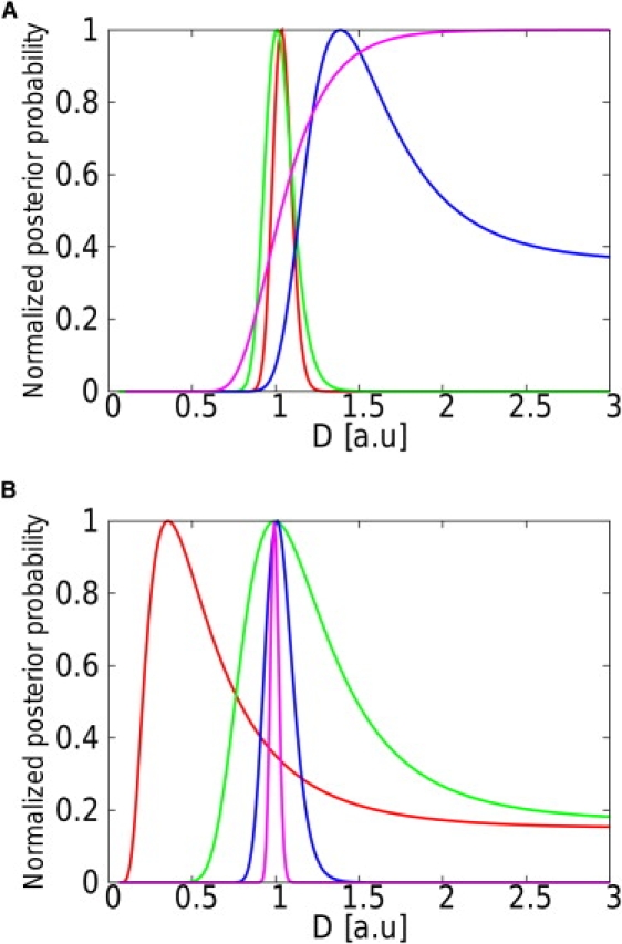
Representation of the evolution of the posterior probability with D for different realizations of the random walk confined in a square domain. The simulations were performed with $\tilde{D}=1$ a.u. (A) Evolution of the posterior probability for different levels of confinement u (u = 0.5, purple; u = 0.25, blue; u = 0.2, green; u = 0.1, red) and a given number of steps (N = 10³). These levels of confinement would be obtained in experiments with D = 0.05 μm².s⁻¹, L = 100 nm, and, respectively, Δt = 100 ms, Δt = 50 ms, Δt = 40 ms, and Δt = 20 ms. (B) Evolution of the posterior probability for different numbers of steps (N = 10, red; N = 100, green; N = 1000, blue; N = 10,000, purple) and a fixed level of confinement (u = 0.2). Realistic experimental parameter values corresponding to this level of confinement could be D = 0.05 μm².s⁻¹, L = 100 nm, and Δt = 40 ms. The $\frac{1}{\sqrt{N}}$ convergence of the estimation toward the actual value of the diffusivity is observed.

Figure 1.

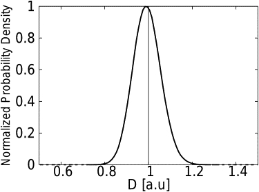
Normalized distribution of the estimates D^∗, common to the MAP and MSD estimators, for free Brownian motion. Trajectories of 500 steps were generated with a time interval Δt = 1 a.u. and an actual diffusivity $\tilde{D}=1$ a.u. The vertical black line is positioned at the mean value of the estimates of diffusivity which is equal to the input value for the generation of the numerical trajectories. Both estimators are unbiased.

Figure 6.

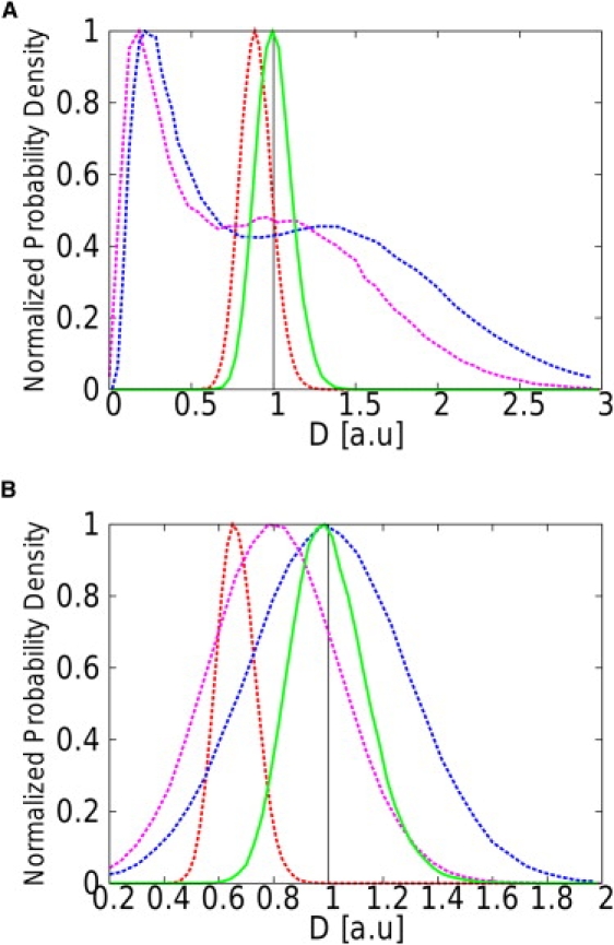
Normalized distributions of the estimations $D_{\text{MSD}}^{\left(1\right)}$, $D_{\text{MSD}}^{\left(2\right)}$, $D_{\text{MSD}}^{\left(3\right)}$, and D_MAP made using the four studied estimators for N = 100 steps and two different values of the confinement level: u = 0.005 (A) and u = 0.05 (B). (MAP estimator, solid green lines; MSD⁽¹⁾, dashed red lines; MSD⁽²⁾, dashed blue; and MSD⁽³⁾, dashed purple.) The vertical black line is positioned at the actual value of the diffusivity ($\tilde{D}=1$ a.u.). The MSD estimators are either biased or less efficient than the MAP estimator.

Figure 7.

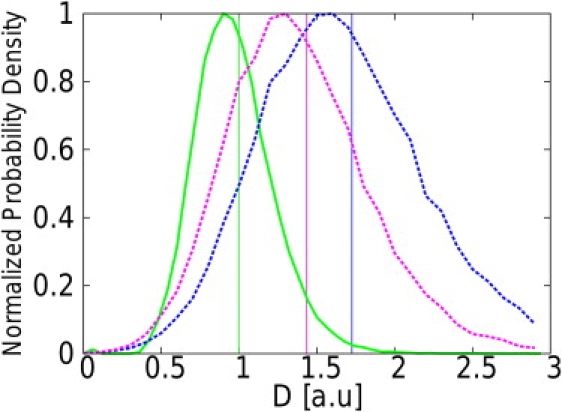
Normalized distributions of D_MAP, $D_{\text{MSD}}^{\left(2\right)}$, and $D_{\text{MSD}}^{\left(3\right)}$ estimates obtained from 10⁵ trajectories with a confinement level u = 0.05 and a noise with standard deviation σ = 0.15 a.u. The trajectories were generated with a diffusivity $\tilde{D}=1$ a.u., L = 1 a.u., Δt = 0.05 a.u., and N = 100 steps. For such a level of confinement, realistic experimental parameter values would be D = 0.05 μm².s⁻¹, L = 100 nm, and Δt = 10 ms. The precision on the position would then be σ = 15 nm. This noise level corresponds to a relative uncertainty of 50% on the position of the particle with respect to the mean one-dimensional displacement $\sqrt{2D\Delta t}$. (MAP estimator, solid green line; $D_{\text{MSD}}^{\left(2\right)}$, dashed blue; and $D_{\text{MSD}}^{\left(3\right)}$, dashed purple.) A vertical line is positioned at the mean value of the distribution with the corresponding color. The distributions of $D_{\text{MSD}}^{\left(2\right)}$ and $D_{\text{MSD}}^{\left(3\right)}$ are shifted toward higher values of the diffusivity under the effect of noise.

Application to experimental data

For experimental trajectories, one should first choose a model of motion. In cases of long trajectories, which are now commonly available thanks to different types of nanoparticles, the membrane molecule fully explores the confining domain and its geometry is clearly visible from the experimental trajectory. In the Supporting Material, the sensitivity of the method to the geometry of the confining domain is studied and can be used to compare the accuracy of different models of motion using Bayesian analysis tools (16). Ideally, after having loaded an experimental trajectory and experimental parameters such as the level of noise, a software adequate to the task could perform estimations of the diffusivity via different Bayesian estimators corresponding to different models of motion (i.e., free diffusion, diffusion confined in domains of different geometries, diffusion within a potential (17)) and their corresponding accuracy.

A Bayesian Estimator

In most single particle experiments, the position $\overrightarrow{r}$ of the particle is detected with time interval Δt. We denote as ${\overrightarrow{r}}_i$ the position of the particle after i time steps. After N time steps, the detected trajectory can be written ${\mathit{R}}_N=\left\{\left({\overrightarrow{r}}_0,t_0\right),\left({\overrightarrow{r}}_1,t_1\right),\dots ,\left({\overrightarrow{r}}_N,t_N\right)\right\}$. The approach that we describe here assumes that the observed motion is a realization R of a stochastic process depending on a set θ of parameters. We denote by W(R|θ) the likelihood of the trajectory according to the stochastic model. We also define $P\left(\overrightarrow{r},t|{\overrightarrow{r}}_0,t_0\right)$ as the transition probability to arrive at the space-time point $\left(\overrightarrow{r},t\right)$ conditional to the initial space-time position $\left({\overrightarrow{r}}_0,t_0\right)$. This transition probability is a function of the set of parameters θ. For a Markovian process, the probability of a realization after N time steps (R_N) can be factorized,

$$W\left({\mathit{R}}_N|\mathit{\theta }\right)=W\left({\overrightarrow{r}}_0,t_0\right)\prod _{i=1}^{N}P\left({\overrightarrow{r}}_i,t_i|{\overrightarrow{r}}_{i-1},t_{i-1}\right),$$ (1)

where $W\left({\overrightarrow{r}}_0,t_0\right)$ is the absolute probability of finding the particle initially at space-time position $\left({\overrightarrow{r}}_0,t_0\right)$.

Bayes' rule links the probability of having a set of parameters θ given a trajectory realization R, P(θ|R) (the posterior probability of the set of parameters), to the likelihood of the trajectory as

$$P\left(\mathit{\theta }|\mathit{R}\right)=\frac{W\left(\mathit{R}|\mathit{\theta }\right)\times P_0\left(\mathit{\theta }\right)}{P\left(\mathit{R}\right)},$$ (2)

where P(R) is a normalizing constant and P₀(θ) is the prior probability that is taken as uniform. Then, one may estimate the set of parameters governing the motion as the set for which the posterior probability reaches its maximum. The corresponding estimator is called the maximum a posteriori (MAP) estimator and is denoted here as T_MAP. For a realization R, the estimation of the parameters via this estimator is then written θ_MAP = T_MAP (R).

Criteria to compare estimators

Other estimators may also be used. For diffusive processes, an estimation of the diffusivity is often made using the MSD. It is then necessary to establish criteria to decide which estimator is preferable. The choice of a given estimator should be driven by its behavior over the whole set of possible realizations. Indeed, a valid estimator should provide estimations that, when averaged over the whole set of possible realizations, give the actual value of the parameter. Such estimators are said to be unbiased. Another important criterion to evaluate the quality of an estimator T is its standard deviation σ(T), equal to the standard deviation of the estimations (over the set of all possible realizations) made using this estimator. The Cramér-Rao inequality states that the standard deviation of any unbiased estimator T_u is lower-bounded (49),

$$\mathit{\sigma }\left(T_u\right)\ge J^{-\frac{1}{2}}\left(\mathit{\theta }\right),$$ (3)

with the equality holding for efficient estimators. J(θ) is the Fisher information, defined as (49)

$$J\left(\mathit{\theta }\right)=\langle {\left({\partial }_{\mathit{\theta }}\text{ln}P\left(\mathit{\theta }|\mathit{R}\right)\right)}^2\rangle ,$$ (4)

the average being performed over the set of all possible realizations. Estimations made using an unbiased and efficient estimator are then guaranteed to provide the best estimates of the set of parameters θ. One should then seek such estimators.

For a Markov process, the Fisher information for N-step realizations can be written in terms of the Fisher information for one-step realizations (49), J_N(θ) = NJ₁(θ).

The standard deviation of the estimations made via any unbiased and efficient estimator T^∗ based on N-step realizations of a Markov process, thus reads

$${\mathit{\sigma }}_{\text{N}}\left(T^{\ast }\right)=\frac{1}{\sqrt{N{J}_1\left(\mathit{\theta }\right)}},$$ (5)

where

$$J_1\left(\mathit{\theta }\right)=\underset{{\mathit{R}}_1\in R_1}{\int }D{\mathit{R}}_{1}P\left(\mathit{\theta }|{\mathit{R}}_1\right){\left({\partial }_{\mathit{\theta }}\text{ln}P\left(\mathit{\theta }|{\mathit{R}}_1\right)\right)}^2\text{.}$$ (6)

R₁ is the set of all possible displacements during one time step. Note that the error of the estimation decreases as the inverse of $\sqrt{N}$, which is as expected from a central limit argument.

Free Brownian Motion

In this section, we compare the MAP estimator and the MSD estimator when the underlying process is free Brownian motion. The only parameter on which the movement depends is the diffusivity D and the transition probability obeys the diffusion equation,

$${\partial }_{t}P=D\Delta P,$$ (7)

whose fundamental solution reads

$$P\left(\overrightarrow{r},t|{\overrightarrow{r}}_0,t_0\right)=\frac{1}{{\left(4\pi D\left(t-t_0\right)\right)}^{\frac{d}{2}}}{e}^{-\frac{{\left(\overrightarrow{r}-{\overrightarrow{r}}_0\right)}^2}{4D\left(t-t_0\right)}},$$ (8)

where d is the space dimension. Because the process is Markovian, we obtain the posterior probability of a diffusivity D given an N-step trajectory R_N via Eqs. 1 and 2,

$$P\left(D|{\mathit{R}}_N\right)\propto \frac{1}{D^{\frac{Nd}{2}}}{e}^{-\frac{1}{4D\Delta t}\sum _{i=0}^{N-1}{\left({\overrightarrow{\text{r}}}_{i+1}-{\overrightarrow{\text{r}}}_i\right)}^2,}$$ (9)

whose maximum is reached for

$$D_{\text{MAP}}=\frac{1}{2\Delta t}\frac{1}{Nd}\sum _{i=0}^{N-1}{\left({\overrightarrow{r}}_{i+1}-{\overrightarrow{r}}_i\right)}^2=D_{\text{MSD}}\text{.}$$ (10)

We see that for any realization of the Brownian motion, the estimations of the diffusivity via the MAP estimator and the MSD estimator are equal, as was also found in Montiel et al. (18). We call D^∗ the common estimate of the diffusivity. Using the Markov property again, one gets 〈D^∗〉 = D and ${\mathit{\sigma }}_{D^{\ast },N}^2=\langle D^{\ast }\rangle -{\langle D^{\ast }\rangle }^2=2D^2/Nd$, the average being performed over the set of all possible N-step realizations. Furthermore, the Fisher information for one-step realizations is

$$J_1\left(D\right)=\frac{d}{2D^2},$$ (11)

thus, the equality in Eq. 3 holds and both MAP and MSD estimators are unbiased and efficient. This means that a better estimate of the diffusivity for free Brownian motion cannot be found. In Fig. 1, we show the distribution of the common estimates D^∗ for numerical trajectories of 500 steps generated with a time step Δt = 1 a.u. and an actual diffusivity $\tilde{D}=1$ a.u. Note that the distribution both here and in figures following is normalized so that its maximum value equals one.

Confined Diffusion

The equivalence between MAP and MSD, valid for free diffusion, does not hold for diffusion confined in a domain as we show here. We consider two-dimensional diffusion confined in a domain of area S defined by its boundary Σ with strictly reflective boundary conditions during the time of the experiment. As in the case of free Brownian motion, we are interested in comparing the accuracy of the estimations of the diffusivity made using MAP and MSD estimators. Between two successive detections of the particle, the typical displacement $\Vert \mathit{\delta }\overrightarrow{r}\Vert$ is ∼$\sqrt{D\Delta t}$. When $\Vert \mathit{\delta }\overrightarrow{r}\Vert$ is comparable to the typical length $\sqrt{S}$ of the domain, the particle will frequently bounce on the domain boundary. We thus introduce a dimensionless parameter, u, that provides a qualitative sense of the level of confinement of the motion,

$$u=\frac{D\Delta t}{S}\text{.}$$ (12)

When u ≃ 1, the particle is likely to bounce at the domain boundary during one time step whereas, when u ≪ 1, the chances for encountering the boundary during one time step are low and the particle will seem to undergo free diffusion on sufficiently short timescales. Fig. 2 gives examples of displacements obtained for u ranging from 10⁻⁴ to 1 in a square domain.

Figure 2.

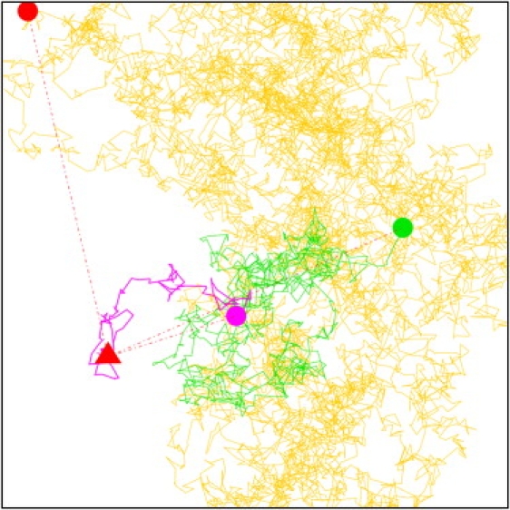
A random walk confined in a square domain. The parameters D, L, and Δt were chosen so that u = 10⁻⁴. The total number of steps is 10⁴. The start position is represented as a red triangle. The first 10² steps are colored in purple (the last point is shown as a purple circle), the next 900 steps are colored in green (last point shown as a green circle), and the rest of the trajectory is colored in yellow with the very last point depicted as a red circle. The displacements connecting the red triangle to the purple, green, and red circles thus illustrate displacements that would be observed for 100Δt (u = 10⁻²), for 10³Δt (u = 0.1), and for 10⁴Δt (u = 1), respectively. These levels of confinement could correspond to experiments where, for instance, D = 0.05 μm².s⁻¹, L = 100 nm, and, respectively, Δt = 0.02 ms (u = 10⁻⁴), Δt = 2 ms (u = 10⁻²), Δt = 20 ms (u = 0.1), and Δt = 200 ms (u = 1).

Evaluation of the transition probability

In the case of confined diffusion, the transition probability $P\left(\overrightarrow{r},t|{\overrightarrow{r}}_0,t_0\right)$ to arrive at the space-time point $\left(\overrightarrow{r},t\right)$ conditional to the initial space-time position $\left({\overrightarrow{r}}_0,t_0\right)$ still obeys the diffusion equation (Eq. 7), but it must also verify the boundary conditions,

$$\overrightarrow{\mathrm{\nabla }}P\left(\overrightarrow{r},t|{\overrightarrow{r}}_0,t_0\right)·\overrightarrow{n}{|}_{\Sigma }=0,$$ (13)

$\overrightarrow{n}$ being the vector normal to the boundary. If one looks for solutions by separating spatial and temporal variables, $\varphi \left(\overrightarrow{r}\right)\chi \left(t\right)$, the problem appears as an eigenvalue problem for functions χ and ϕ (51),

$${\partial }_t\chi =-{\gamma }^{2}D\chi ,\Delta \varphi =-{\gamma }^2\varphi ,$$ (14)

γ being a real constant. The general solution for χ reads $\chi \left(t\right)=\chi \left(0\right)e^{-{\gamma }^{2}Dt}$. For spatial variables, the general solution is expressed as the superposition of the different eigenfunctions ϕ_{γ, i} of the Laplace operator Δ for the eigenvalue γ². Note that the index i of the eigenfunctions corresponds to the case where the eigenvalue, γ², is degenerate. Thus, the transition probability can be written

$$P\left(\overrightarrow{r},t|{\overrightarrow{r}}_0,t_0\right)=\sum _{\gamma ,i}{A}_{\gamma ,i}\left({\overrightarrow{r}}_0,t_0\right){\mathit{\varphi }}_{\gamma ,i}\left(\overrightarrow{r}\right)e^{-{\mathit{\gamma }}^{2}Dt}\text{.}$$ (15)

Boundary conditions then lead to the quantification of the possible values of constant γ and $A_{\gamma ,\text{i}}\left({\overrightarrow{r}}_0,t_0\right)$ is given by the initial condition ${\text{lim}}_{\text{t}\to {\text{t}}_0}P\left(\overrightarrow{r},t|{\overrightarrow{r}}_0,t_0\right)=\mathit{\delta }\left(\overrightarrow{r},{\overrightarrow{r}}_0\right)$. In the Supporting Material, we expose the transition probabilities corresponding to most of the geometries that may be encountered in applications (square, rectangular, circular, and elliptic).

Evaluation of the lowest achievable uncertainty

Once the transition probability is known, it is possible to derive the Fisher information, J₁(D). We can write this quantity in terms of the dimensionless parameter u, as

$$J_1\left(D\right)=\frac{D^2}{u^2}{J}_1\left(u\right)\text{.}$$ (16)

Then, for any unbiased and efficient estimator of the diffusivity T^∗, the standard deviation of the estimations over the set of N steps realizations R_N is

$${\mathit{\sigma }}_N\left(T^{\ast }\right)={\mathit{\sigma }}^{\ast }=\frac{D}{u\sqrt{N{J}_1\left(u\right)}}\text{.}$$ (17)

The lowest achievable relative uncertainty of the estimations, which we shall denote as η, can be expressed as

$$\eta =\frac{{\sigma }^{\ast }}{D}=\frac{1}{u\sqrt{N{J}_1\left(u\right)}}\text{.}$$ (18)

J₁(u) is obtained by an averaging process over all the possible displacements during one time step and therefore depends only on the geometry of the confining domain.

For high confinement, J₁(u) is well approximated by the asymptotic expression

$$J_1\left(u\right)\mathrm{\propto }{\text{e}}^{-\beta \text{u}}\text{.}$$ (19)

For square domains, β = 2π². For rectangular domains of size L × W with L > W, u is defined by $D\Delta t/L.W$ and $\mathit{\beta }=2\frac{W}{L}{\pi }^2$. For circular domains of radius a, $u=D\Delta t/\pi a^2$ and $\beta =2k_{1,1}^2\pi$, k_{1, 1} being the first zero of the first derivative of the Bessel function of order one (k_{1, 1} ≈ 1.841). For elliptic domains with major axis a and minor axis b, $u=D\Delta t/\pi ab$ and $\beta =4k_{0,1,c}^{{\xi }_a}\pi \frac{ab}{a^2-b^2}$ with $k_{0,1,c}^{{\xi }_a}$ defined in the Supporting Material. For high confinement, the number of data points necessary to achieve a given precision grows dramatically with u. When confinement is low, the free Brownian diffusion approximation is reasonable and $J_1\left(u\right)\sim \frac{1}{u^2}$ (d = 2 in Eq. 11), giving

$$\eta \sim \frac{1}{\sqrt{N}}\text{.}$$ (20)

For intermediate confinement, J₁(u) should be computed numerically. It is important to note that J₁(u) is nonzero for all u. Thus, η is finite, which means that there are no theoretical limitations to achieve any precision provided one is able to collect a sufficient amount of data points. The number of points necessary, however, grows dramatically with u for high confinement as shown in Fig. 3.

Figure 3.

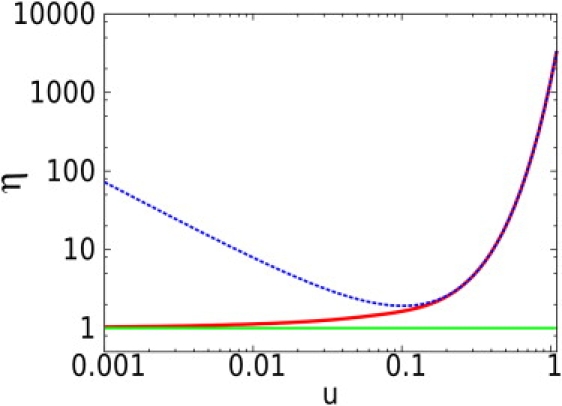
Representation in log-log scale of the evolution of the lowest achievable relative uncertainty η (solid red line) with respect to the confinement u for a square domain and N = 1. The figure also shows asymptotic approximations for free diffusion (solid green line) and high confinement (dashed blue line), exhibiting the dramatic increase of the uncertainty for high confinement. Note that to obtain the evolution of η for N > 1, a factor $\frac{1}{2}\text{log}\left(N\right)$ needs to be subtracted.

MAP estimations of the diffusivity

Knowing the transition probability also allows the estimation of the diffusivity via the MAP estimator. For the sake of simplicity, we will focus here on the square geometry but the same behavior was observed for all other geometries studied. For a square domain of size L × L, the confinement parameter previously introduced is $u=\text{D}\Delta \text{t}/{\text{L}}^2$. The posterior probability of the diffusivity D given an N-step realization R_N reads

$$P\left(D|{\mathit{R}}_N\right)=\frac{1}{L^2}\prod _{i=1}^{N}P\left({\overrightarrow{r}}_i,t_i|{\overrightarrow{r}}_{i-1},t_{i-1}\right)\text{.}$$ (21)

$P\left({\overrightarrow{r}}_i,t_i|{\overrightarrow{r}}_{i-1},t_{i-1}\right)$ is calculated according to the results exposed in the Supporting Material. We generated an N-step random walk R_N with diffusivity $\tilde{D}$ = 1 arbitrary unit (a.u.), L = 1 a.u., and Δt was chosen according to the desired value of the confinement parameter u. It is then possible to plot the posterior probability as a function of D. The MAP estimate D_MAP of the diffusivity is the value of D for which the maximum is reached. Fig. 4 A shows some of these plots for different levels of confinement and a fixed number of steps (N = 10³). For sufficiently low levels of confinement, D_MAP is close to the actual diffusivity $\tilde{D}$, whereas the estimation becomes less accurate as u increases—which is as expected from the evolution of η in Fig. 3. For the case u = 0.5, we see that no maximum of the posterior probability is found. The MAP estimator can be considered biased for this set of parameters (u = 0.5 and N = 10³) and no accurate estimation of the diffusivity can therefore be achieved. For such parameters, J₁(0.5) ≃ 0.01 and $\frac{1}{\sqrt{N{u}^2{J}_1\left(u\right)}}$ ≃ 0.63. Therefore, according to Eq. 18, no estimation can be performed with <63% error. Nevertheless, if the number of steps increases sufficiently, the posterior probability will eventually exhibit a maximum, thus allowing a proper estimation of the diffusivity. Indeed, extensive simulations strongly support the assumption that the MAP estimator is unbiased and efficient, provided a maximum of the posterior probability exists for a finite value of D for every realization as shown in Fig. 5. The number of steps needed to achieve a desired precision should therefore be estimated using Eq. 18. In this particular case (u = 0.5 and N = 10³), ∼4 × 10⁴ steps would be required to estimate D with 10% error. The evolution of the posterior probability with respect to the number of steps is illustrated in Fig. 4 B for a simulation performed with u = 0.2 and N ranging from 10 to 10⁴. The diffusivity used for the simulation was chosen to be $\tilde{D}$ = 1 a.u. The posterior probability already peaks very close to this value for N = 100 and the peak gets sharper and sharper as N increases. The standard deviation of the estimations decreases as $\frac{1}{\sqrt{\text{N}}}$ as stated by Eq. 18. For N = 10⁴ the relative error on the estimation is then close to 2.5%. Similar behaviors were obtained for all the domain geometries studied.

Figure 5.

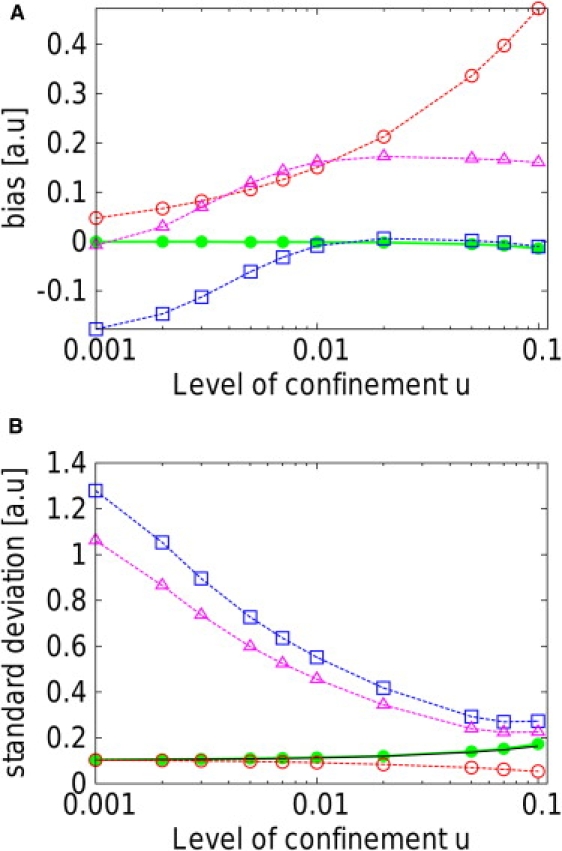
Representation of the bias (A) and standard deviation (B) of the MAP and MSD estimators with respect to the level of confinement u, for N = 100 time steps. For each u, ∼10⁵ trajectories were used to evaluate these quantities. (MAP estimator, solid green lines; MSD⁽¹⁾, dashed red lines; MSD⁽²⁾, dashed blue; and MSD⁽³⁾, dashed purple.) The bias is defined as the difference between the actual value of the diffusivity used in the simulations ($\tilde{D}=1$ a.u.) and the average value of the estimations made using a given estimator. Only the MAP estimator is unbiased over the whole range of levels of confinement. The lowest achievable standard deviation of the estimations, the Cramér-Rao bound, is represented as the solid black line. The performances of the MAP estimator are practically identical to the theoretical Cramér-Rao bound. All MSD estimators are either largely biased or less efficient than the MAP estimator.

Comparison of MAP and MSD estimators

The MSD after n time steps reads

$$\text{MSD}\left(n\Delta t\right)=\frac{1}{\left(N-n\right)}\sum _{i=0}^{N-1-n}{\left({\overrightarrow{r}}_{i+n}-{\overrightarrow{r}}_i\right)}^2\text{.}$$ (22)

For two-dimensional free Brownian motion, we have seen that we can estimate the diffusivity via

$$D_{\text{MSD}}^{\left(1\right)}=\frac{1}{4\Delta t}\text{MSD}\left(\Delta t\right),$$ (23)

and that this method of estimation achieves the lowest possible uncertainty on the diffusivity. We will shortly see that this is no longer the case when the motion is confined. For a random walk of diffusivity D confined in a square domain of size L × L, the expected MSD after n time steps (averaged over all the possible n time step displacements) is (48,52)

$$\langle {\left(\Delta \overrightarrow{r}\left(n\Delta t\right)\right)}^2\rangle =2\left(\frac{L^2}{6}-\frac{16L^2}{{\pi }^4}\sum _{k=1,\left(\text{odd}\right)}^{\mathrm{\infty }}\frac{1}{k^4}{e}^{-{\left(\frac{k\pi }{L}\right)}^{2}Dn\Delta t}\right)\text{.}$$ (24)

The diffusivity can be estimated by least-squares fitting the MSD curve given by Eq. 22 using the previous formula. We denote as $D_{\text{MSD}}^{\left(2\right)}$ the resulting estimate of the diffusivity. The 500 first terms of the sum in Eq. 24 were used in the least-squares fitting procedure. Another method consists in least-squares fitting the two-dimensional MSD curve given by Eq. 22 with the formula $\frac{L^2}{3}\left(1-e^{-\lambda t}\right)$ and the diffusivity is then estimated as $D_{\text{MSD}}^{\left(3\right)}=\frac{\lambda L^2}{12}$ (24).

To compare the quality of the MSD estimates to that of the MAP estimate we generated a large number of confined random walks (∼10⁵) with a given diffusivity $\tilde{D}$ = 1 a.u. For each realization, we obtain a set of estimates of the diffusivity $\left\{D_{\text{MSD}}^{\left(1\right)},D_{\text{MSD}}^{\left(2\right)},D_{\text{MSD}}^{\left(3\right)},D_{\text{MAP}}\right\}$. The bias and the standard deviation of the estimations for each estimator can then be evaluated. In Fig. 5, we plot these quantities with respect to the level of confinement u for N = 100 time steps. For the values of u shown in Fig. 5 and the chosen number of steps N, it was always possible to perform the four estimations (the least-squares functions and the posterior probability all had an extremum for finite values of D). Complete distributions of the estimations made using the three estimators are shown in Fig. 6 for u = 0.005 and u = 0.05. Note that the length L of the domain is considered as known. Similar results, presented in the Supporting Material, are obtained when L has to be estimated along with D.

We see that the first MSD estimator is biased and largely underestimates the diffusivity. As the level of confinement increases, its bias increases. Note that this estimator seems to overcome the theoretical Cramér-Rao lower bound (Fig. 5 B). This is possible only because this estimator is biased. The distribution of the estimations can then be sharply peaked on a underestimated value of the diffusivity as shown in Fig. 6. Note that we only use the first two points of the MSD curve for this first MSD estimator. In experimental work, the first three or five points of the MSD curve are also frequently used to estimate the diffusivity via the initial slope of the MSD curve. In those cases, we have found the bias of the estimation to be even larger. The second and third MSD estimators are also biased for low confinement and, on average, overestimate the diffusivity. However, the second MSD estimator seems to become unbiased for sufficiently high confinement. We also observe that their standard deviations decrease as u increases, but they always exceed the standard deviation of the estimations made using the MAP estimator. The MAP estimator is unbiased in the whole range of levels of confinement studied. Its standard deviation is practically identical to the lowest achievable uncertainty evaluated via Eq. 18. The MAP estimator can then reasonably be considered as unbiased and efficient, provided a maximum of the posterior probability exists for a finite value of D for all possible realizations. In this framework, the maximum of the posterior distribution provides the best theoretically achievable estimate of the diffusivity.

Robustness to Noise

So far, we have assumed that the position of the tracked biomolecule was known exactly. Experimentally, an uncertainty on the position of the particle exists though. We investigate in this section how MAP and MSD estimators are affected by the existence of noise in the position of the particle in the cases of free Brownian motion and confined diffusion. In both cases we assume that the detected position of the particle at time t_i, ${\overrightarrow{r}\prime }_i$, can be obtained from the position of the underlying random walk, ${\overrightarrow{r}}_i$, as ${\overrightarrow{r}\prime }_i={\overrightarrow{r}}_i+\Delta {\overrightarrow{r}}_i$, where each component of $\Delta {\overrightarrow{r}}_i$ is distributed according to a normal law with a known standard deviation σ, N(0,σ). Note that σ is to be determined from the experimental data, for example by using the error bar on the center of the two-dimensional Gaussian that is used to fit the single-molecule signal in the two-dimensional images. With such a Gaussian noise, the probability to detect the particle at ${\overrightarrow{r}\prime }_i$ knowing its actual position is ${\overrightarrow{r}}_i$ reads

$$P\left({\overrightarrow{r}\prime }_i|{\overrightarrow{r}}_i\right)=\frac{1}{{\left(2\pi {\mathit{\sigma }}^2\right)}^{\frac{\text{d}}{2}}}{e}^{-\frac{{\left({\overrightarrow{r}\prime }_i-{\overrightarrow{r}}_i\right)}^2}{2{\mathit{\sigma }}^2}},$$ (25)

where d is the dimension of the random walk. During one time step, the transition probability for the particle to be consecutively detected at positions ${\overrightarrow{r}\prime }_i$ and ${\overrightarrow{r}\prime }_{i+1}$ must now be written as

$$P\left({\overrightarrow{r}\prime }_{i+1},t_i+\Delta t|{\overrightarrow{r}\prime }_i,t_i\right)=\int d{\overrightarrow{r}}_{i}d{\overrightarrow{r}}_{i+1}P\left({\overrightarrow{r}\prime }_{i+1}|{\overrightarrow{r}}_{i+1}\right)P\left({\overrightarrow{r}}_{i+1},t_i+\Delta t|{\overrightarrow{r}}_i,t_i\right)P\left({\overrightarrow{r}\prime }_i|{\overrightarrow{r}}_i\right),$$ (26)

where $P\left({\overrightarrow{r}}_{i+1},t_i+\Delta t|{\overrightarrow{r}}_i,t_i\right)$ is the transition probability for the underlying random walk without noise. Note that the integration has to be performed over all the possible positions ${\overrightarrow{r}}_i$ and ${\overrightarrow{r}}_{i+1}$. We can then approximate the likelihood of the noisy trajectory for N time steps (R′_N) as (50)

$$W\left({\mathit{R}}_N^{\prime }|\mathit{\theta }\right)=W\left({\overrightarrow{r}\prime }_0,t_0\right)\prod _{i=1}^{N}P\left({\overrightarrow{r}\prime }_i,t_i|{\overrightarrow{r}\prime }_{i-1},t_{i-1}\right)$$ (27)

and the posterior probability is given by Bayes' rule (Eq. 2). (Note that the exact solution is a convolution of the likelihood of the trajectory without noise W(R_N|θ) with the product of N + 1 Gaussian laws centered on positions $\left\{{\overrightarrow{r}}_i,i=0..N\right\}$ with standard deviation σ. The integration must be performed over the positions $\left\{{\overrightarrow{r}}_i,i=0..N\right\}$ as in Eq. 26.)

Free Brownian motion

For free Brownian motion, the transition probability in the presence of noise becomes

$$P\left({\overrightarrow{r}\prime }_{i+1},t_i+\Delta t|{\overrightarrow{r}\prime }_i,t_i\right)=\frac{1}{{\left(4\pi D^{\prime }\Delta t\right)}^{\frac{d}{2}}}{e}^{-\frac{{\left({\overrightarrow{r}\prime }_{i+1}-{\overrightarrow{r}\prime }_{\text{i}}\right)}^2}{4D^{\prime }\Delta \text{t}}},$$ (28)

with $D^{\prime }=D+{\mathit{\sigma }}^2/\Delta \text{t}$. The maximum of the posterior probability is then reached for

$$D_{\text{MAP}}=\frac{1}{2\Delta t}\frac{1}{Nd}\sum _{i=0}^{N-1}{\left({\overrightarrow{r}\prime }_{i+1}-{\overrightarrow{r}\prime }_i\right)}^2-\frac{{\mathit{\sigma }}^2}{\Delta t}=D_{\text{MSD}}-\frac{{\mathit{\sigma }}^2}{\Delta t}\text{.}$$ (29)

We see that MAP and MSD estimates of the diffusivity differ when we take into account the noise in the posterior probability. The distributions of the estimations made via the MSD estimator is then shifted toward higher values of diffusivity, in agreement with the findings of Montiel et al. (18). The Gaussian noise can indeed be seen as an independent diffusive process that adds up with the underlying Brownian motion, thus increasing the apparent diffusivity. The MAP estimator corrects this effect as demonstrated for two different noise levels (σ = 0.3 a.u. and σ = 1 a.u.) in Fig. S1. The MAP estimator remains unbiased as the noise level increases. From Eq. 29, it follows that one can also get unbiased estimations of the diffusivity by subtracting a factor ${\mathit{\sigma }}^2/\Delta \text{t}$ from MSD estimations D_MSD.

Confined diffusion

We investigate here the effect of the Gaussian noise on the estimations of the diffusivity when the motion is confined in a square domain of size L × L. The posterior probability can also be approximated in this framework (see Supporting Material) and a MAP estimator taking the noise into account is then defined. We generated 10⁵ trajectories with a diffusivity $\tilde{D}=1$ a.u., L = 1 a.u., and Δt = 0.05 a.u. so that the confinement level is u = 0.05. For such a confinement level, we have seen in Fig. 5 A that both the second MSD estimator (providing estimations $D_{\text{MSD}}^{\left(2\right)}$) and the MAP estimator seem to be unbiased when there is no noise. We add here a noise with standard deviation σ = 0.15 a.u. To take noise into account in the MSD estimations, it is usual to subtract a factor 2σ² from Eq. 22 before performing the least-squares fitting procedures. The modified MSD estimates are still denoted as $D_{\text{MSD}}^{\left(2\right)}$ and $D_{\text{MSD}}^{\left(3\right)}$ in the following. In Fig. 7, we plot the distributions of D_MAP, $D_{\text{MSD}}^{\left(2\right)}$, and $D_{\text{MSD}}^{\left(3\right)}$ estimates obtained with this set of parameters. The distribution of D_MAP is peaked on the actual value of the diffusivity whereas the distributions of $D_{\text{MSD}}^{\left(2\right)}$ and $D_{\text{MSD}}^{\left(3\right)}$ are shifted toward higher values of diffusivity. This shift toward higher diffusivities is also observed if the factor 2σ² is not subtracted from Eq. 22, as described above. The proposed Bayesian scheme thus reveals itself highly robust to noise on the position of the biomolecule.

Conclusions

In this article, we have presented a systematic Bayesian scheme to estimate the diffusivity of a biomolecule. For an assumed model of motion, the posterior probability of the parameter can be determined exactly or approximated using the maximum posterior estimator. In the framework of free Brownian motion and confined diffusion within a domain with strictly reflective boundary conditions, this estimator is shown to reach the best performances theoretically achievable according to the Cramér-Rao limit. As a consequence, the uncertainty on the estimation is provided. Furthermore, the number of data points necessary to achieve any desired precision can easily be estimated. Other estimators making use of an analysis of the MSD are shown to be either biased or less efficient. The Bayesian estimator has also been shown to be highly robust to noise on the position of the biomolecule in both frameworks. For more complex models of motion such as diffusion within a confining potential, the relevance of such a Bayesian scheme has also been demonstrated (17). Accurate descriptions of biomolecule dynamics can thus be provided using such Bayesian methods.

Supporting Material

Additional text, equations, references, and three figures are available at http://www.biophysj.org/biophysj/supplemental/S0006-3495(09)01726-3.

References

- 1.Saxton M.J., Jacobson K. Single-particle tracking: applications to membrane dynamics. Annu. Rev. Biophys. Biomol. Struct. 1997;26:373–399. doi: 10.1146/annurev.biophys.26.1.373. [DOI] [PubMed] [Google Scholar]
- 2.Schütz G.J., Schindler H., Schmidt T. Single-molecule microscopy on model membranes reveals anomalous diffusion. Biophys. J. 1997;73:1073–1080. doi: 10.1016/S0006-3495(97)78139-6. [DOI] [PMC free article] [PubMed] [Google Scholar]
- 3.Lommerse P.H., Blab G.A., Schmidt T. Single-molecule imaging of the H-Ras membrane-anchor reveals domains in the cytoplasmic leaflet of the cell membrane. Biophys. J. 2004;86:609–616. doi: 10.1016/S0006-3495(04)74139-9. [DOI] [PMC free article] [PubMed] [Google Scholar]
- 4.Hebert B., Costantino S., Wiseman P.W. Spatiotemporal image correlation spectroscopy (STICS) theory, verification, and application to protein velocity mapping in living CHO cells. Biophys. J. 2005;88:3601–3614. doi: 10.1529/biophysj.104.054874. [DOI] [PMC free article] [PubMed] [Google Scholar]
- 5.Semrau S., Schmidt T. Particle image correlation spectroscopy (PICS): retrieving nanometer-scale correlations from high-density single-molecule position data. Biophys. J. 2007;92:613–621. doi: 10.1529/biophysj.106.092577. [DOI] [PMC free article] [PubMed] [Google Scholar]
- 6.Condamin S., Tejedor V., Klafter J. Probing microscopic origins of confined subdiffusion by first-passage observables. Proc. Natl. Acad. Sci. USA. 2008;105:5675–5680. doi: 10.1073/pnas.0712158105. [DOI] [PMC free article] [PubMed] [Google Scholar]
- 7.Schuster J., Cichos F., von Borczyskowski C. Diffusion measurements by single-molecule spot-size analysis. J. Phys. Chem. A. 2002;106:5403–5406. [Google Scholar]
- 8.Coscoy S., Huguet E., Amblard F. Statistical analysis of sets of random walks: how to resolve their generating mechanism. Bull. Math. Biol. 2007;69:2467–2492. doi: 10.1007/s11538-007-9227-8. [DOI] [PubMed] [Google Scholar]
- 9.Jin S., Haggie P.M., Verkman A.S. Single-particle tracking of membrane protein diffusion in a potential: simulation, detection, and application to confined diffusion of CFTR Cl− channels. Biophys. J. 2007;93:1079–1088. doi: 10.1529/biophysj.106.102244. [DOI] [PMC free article] [PubMed] [Google Scholar]
- 10.Wieser S., Axmann M., Schütz G.J. Versatile analysis of single-molecule tracking data by comprehensive testing against Monte Carlo simulations. Biophys. J. 2008;95:5988–6001. doi: 10.1529/biophysj.108.141655. [DOI] [PMC free article] [PubMed] [Google Scholar]
- 11.Saxton M.J. Lateral diffusion in an archipelago. Single-particle diffusion. Biophys. J. 1993;64:1766–1780. doi: 10.1016/S0006-3495(93)81548-0. [DOI] [PMC free article] [PubMed] [Google Scholar]
- 12.Simson R., Sheets E.D., Jacobson K. Detection of temporary lateral confinement of membrane proteins using single-particle tracking analysis. Biophys. J. 1995;69:989–993. doi: 10.1016/S0006-3495(95)79972-6. [DOI] [PMC free article] [PubMed] [Google Scholar]
- 13.Saxton M.J. Single-particle tracking: models of directed transport. Biophys. J. 1994;67:2110–2119. doi: 10.1016/S0006-3495(94)80694-0. [DOI] [PMC free article] [PubMed] [Google Scholar]
- 14.Bouzigues C., Dahan M. Transient directed motions of GABAA receptors in growth cones detected by a speed correlation index. Biophys. J. 2007;92:654–660. doi: 10.1529/biophysj.106.094524. [DOI] [PMC free article] [PubMed] [Google Scholar]
- 15.Jin S., Verkman A.S. Single particle tracking of complex diffusion in membranes: simulation and detection of barrier, raft, and interaction phenomena. J. Phys. Chem. B. 2007;111:3625–3632. doi: 10.1021/jp067187m. [DOI] [PubMed] [Google Scholar]
- 16.Mackay D.J.C. Cambridge University Press; West Nyack, NY: 2003. Information Theory, Inference, and Learning Algorithms. [Google Scholar]
- 17.Masson J.-B., Casanova D., Alexandrou A. Inferring maps of forces inside cell membrane microdomains. Phys. Rev. Lett. 2009;102:048103. doi: 10.1103/PhysRevLett.102.048103. [DOI] [PubMed] [Google Scholar]
- 18.Montiel D., Cang H., Yang H. Quantitative characterization of changes in dynamical behavior for single-particle tracking studies. J. Phys. Chem. B. 2006;110:19763–19770. doi: 10.1021/jp062024j. [DOI] [PubMed] [Google Scholar]
- 19.Qian H., Sheetz M.P., Elson E.L. Single particle tracking. Analysis of diffusion and flow in two-dimensional systems. Biophys. J. 1991;60:910–921. doi: 10.1016/S0006-3495(91)82125-7. [DOI] [PMC free article] [PubMed] [Google Scholar]
- 20.Saxton M.J. Single-particle tracking: the distribution of diffusion coefficients. Biophys. J. 1997;72:1744–1753. doi: 10.1016/S0006-3495(97)78820-9. [DOI] [PMC free article] [PubMed] [Google Scholar]
- 21.Daumas F., Destainville N., Salomé L. Confined diffusion without fences of a g-protein-coupled receptor as revealed by single particle tracking. Biophys. J. 2003;84:356–366. doi: 10.1016/S0006-3495(03)74856-5. [DOI] [PMC free article] [PubMed] [Google Scholar]
- 22.Ritchie K., Shan X.Y., Kusumi A. Detection of non-Brownian diffusion in the cell membrane in single molecule tracking. Biophys. J. 2005;88:2266–2277. doi: 10.1529/biophysj.104.054106. [DOI] [PMC free article] [PubMed] [Google Scholar]
- 23.Suzuki K., Ritchie K., Kusumi A. Rapid hop diffusion of a G-protein-coupled receptor in the plasma membrane as revealed by single-molecule techniques. Biophys. J. 2005;88:3659–3680. doi: 10.1529/biophysj.104.048538. [DOI] [PMC free article] [PubMed] [Google Scholar]
- 24.Destainville N., Salomé L. Quantification and correction of systematic errors due to detector time-averaging in single-molecule tracking experiments. Biophys. J. 2006;90:L17–L19. doi: 10.1529/biophysj.105.075176. [DOI] [PMC free article] [PubMed] [Google Scholar]
- 25.Ober R.J., Ram S., Ward E.S. Localization accuracy in single-molecule microscopy. Biophys. J. 2004;86:1185–1200. doi: 10.1016/S0006-3495(04)74193-4. [DOI] [PMC free article] [PubMed] [Google Scholar]
- 26.Ram S., Ward E.S., Ober R.J. Beyond Rayleigh's criterion: a resolution measure with application to single-molecule microscopy. Proc. Natl. Acad. Sci. USA. 2006;103:4457–4462. doi: 10.1073/pnas.0508047103. [DOI] [PMC free article] [PubMed] [Google Scholar]
- 27.Martin D.S., Forstner M.B., Käs J.A. Apparent subdiffusion inherent to single particle tracking. Biophys. J. 2002;83:21092117. doi: 10.1016/S0006-3495(02)73971-4. [DOI] [PMC free article] [PubMed] [Google Scholar]
- 28.Singer S.J., Nicolson G.L. The fluid mosaic model of the structure of cell membranes. Science. 1972;175:720–731. doi: 10.1126/science.175.4023.720. [DOI] [PubMed] [Google Scholar]
- 29.Simons K., Ikonen E. Functional rafts in cell membranes. Nature. 1997;387:569–572. doi: 10.1038/42408. [DOI] [PubMed] [Google Scholar]
- 30.Simons K., Toomre D. Lipid rafts and signal transduction. Nat. Rev. Mol. Cell. Biol. 2000;1:31–39. doi: 10.1038/35036052. [DOI] [PubMed] [Google Scholar]
- 31.Sheets E.D., Lee G.M., Jacobson K. Transient confinement of a glycosylphosphatidylinositol-anchored protein in the plasma membrane. Biochemistry. 1997;36:12449–12458. doi: 10.1021/bi9710939. [DOI] [PubMed] [Google Scholar]
- 32.Varma R., Mayor S. GPI-anchored proteins are organized in submicron domains at the cell surface. Nature. 1998;394:798–801. doi: 10.1038/29563. [DOI] [PubMed] [Google Scholar]
- 33.Simson R., Yang B., Jacobson K.A. Structural mosaicism on the submicron scale in the plasma membrane. Biophys. J. 1998;74:297–308. doi: 10.1016/S0006-3495(98)77787-2. [DOI] [PMC free article] [PubMed] [Google Scholar]
- 34.Pralle A., Keller P., Hörber J.K. Sphingolipid-cholesterol rafts diffuse as small entities in the plasma membrane of mammalian cells. J. Cell Biol. 2000;148:997–1008. doi: 10.1083/jcb.148.5.997. [DOI] [PMC free article] [PubMed] [Google Scholar]
- 35.Schütz G.J., Kada G., Schindler H. Properties of lipid microdomains in a muscle cell membrane visualized by single molecule microscopy. EMBO J. 2000;19:892–901. doi: 10.1093/emboj/19.5.892. [DOI] [PMC free article] [PubMed] [Google Scholar]
- 36.Dietrich C., Yang B., Jacobson K. Relationship of lipid rafts to transient confinement zones detected by single particle tracking. Biophys. J. 2002;82:274–284. doi: 10.1016/S0006-3495(02)75393-9. [DOI] [PMC free article] [PubMed] [Google Scholar]
- 37.Zacharias D.A., Violin J.D., Tsien R.Y. Partitioning of lipid-modified monomeric GFPs into membrane microdomains of live cells. Science. 2002;296:913–916. doi: 10.1126/science.1068539. [DOI] [PubMed] [Google Scholar]
- 38.Marguet D., Lenne P.F., He H.T. Dynamics in the plasma membrane: how to combine fluidity and order. EMBO J. 2006;25:3446–3457. doi: 10.1038/sj.emboj.7601204. [DOI] [PMC free article] [PubMed] [Google Scholar]
- 39.Eggeling C., Ringemann C., Hell S.W. Direct observation of the nanoscale dynamics of membrane lipids in a living cell. Nature. 2009;457:1159–1162. doi: 10.1038/nature07596. [DOI] [PubMed] [Google Scholar]
- 40.Tomishige M., Sako Y., Kusumi A. Regulation mechanism of the lateral diffusion of band 3 in erythrocyte membranes by the membrane skeleton. J. Cell Biol. 1998;142:989–1000. doi: 10.1083/jcb.142.4.989. [DOI] [PMC free article] [PubMed] [Google Scholar]
- 41.Fujiwara T., Ritchie K., Kusumi A. Phospholipids undergo hop diffusion in compartmentalized cell membrane. J. Cell Biol. 2002;157:1071–1081. doi: 10.1083/jcb.200202050. [DOI] [PMC free article] [PubMed] [Google Scholar]
- 42.Nakada C., Ritchie K., Kusumi A. Accumulation of anchored proteins forms membrane diffusion barriers during neuronal polarization. Nat. Cell Biol. 2003;5:629–632. doi: 10.1038/ncb1009. [DOI] [PubMed] [Google Scholar]
- 43.Murase K., Fujiwara T., Kusumi A. Ultrafine membrane compartments for molecular diffusion as revealed by single molecule techniques. Biophys. J. 2004;86:4075–4093. doi: 10.1529/biophysj.103.035717. [DOI] [PMC free article] [PubMed] [Google Scholar]
- 44.Kusumi A., Nakada C., Fujiwara T. Paradigm shift of the plasma membrane concept from the two-dimensional continuum fluid to the partitioned fluid: high-speed single-molecule tracking of membrane molecules. Annu. Rev. Biophys. Biomol. Struct. 2005;34:351–378. doi: 10.1146/annurev.biophys.34.040204.144637. [DOI] [PubMed] [Google Scholar]
- 45.Umemura Y.M., Vrljic M., Kusumi A. Both MHC class II and its GPI-anchored form undergo hop diffusion as observed by single-molecule tracking. Biophys. J. 2008;95:435–450. doi: 10.1529/biophysj.107.123018. [DOI] [PMC free article] [PubMed] [Google Scholar]
- 46.Andrews N.L., Lidke K.A., Lidke D.S. Actin restricts Fc ɛRI diffusion and facilitates antigen-induced receptor immobilization. Nat. Cell Biol. 2008;10:955–963. doi: 10.1038/ncb1755. [DOI] [PMC free article] [PubMed] [Google Scholar]
- 47.Sieber J.J., Willig K.I., Lang T. Anatomy and dynamics of a supramolecular membrane protein cluster. Science. 2007;317:1072–1076. doi: 10.1126/science.1141727. [DOI] [PubMed] [Google Scholar]
- 48.Kusumi A., Sako Y., Yamamoto M. Confined lateral diffusion of membrane receptors as studied by single particle tracking (nanovid microscopy). Effects of calcium-induced differentiation in cultured epithelial cells. Biophys. J. 1993;65:2021–2040. doi: 10.1016/S0006-3495(93)81253-0. [DOI] [PMC free article] [PubMed] [Google Scholar]
- 49.Cover T.M., Thomas J.A. Wiley-Interscience; Hoboken, NJ: 2006. Elements of Information Theory. [Google Scholar]
- 50.Press W.H., Flannery B.P., Vetterling W.T. 2nd ed. Cambridge University Press; West Nyack, NY: 1992. Numerical Recipes in C, The Art of Scientific Computing. [Google Scholar]
- 51.Risken H., Frank T. Springer Series in Synergetics; Springer, New York: 1996. The Fokker-Planck Equation: Methods of Solutions and Applications. [Google Scholar]
- 52.Fourier J. Cosimo; New York: 2007. The Analytical Theory of Heat. [Google Scholar]
Associated Data
This section collects any data citations, data availability statements, or supplementary materials included in this article.