Comparison of the roex and gammachirp filters as representations of the auditory filter

Abstract

Although the rounded-exponential (roex) filter has been successfully used to represent the magnitude response of the auditory filter, recent studies with the roex(p,w,t) filter reveal two serious problems: the fits to notched-noise masking data are somewhat unstable unless the filter is reduced to a physically unrealizable form, and there is no time-domain version of the roex(p,w,t) filter to support modeling of the perception of complex sounds. This paper describes a compressive gammachirp (cGC) filter with the same architecture as the roex(p,w,t) which can be implemented in the time domain. The gain and asymmetry of this parallel cGC filter are shown to be comparable to those of the roex(p,w,t) filter, but the fits to masking data are still somewhat unstable. The roex(p,w,t) and parallel cGC filters were also compared with the cascade cGC filter [Patterson et al., J. Acoust. Soc. Am. 114, 1529–1542 (2003)], which was found to provide an equivalent fit with 25% fewer coefficients. Moreover, the fits were stable. The advantage of the cascade cGC filter appears to derive from its parsimonious representation of the high-frequency side of the filter. It is concluded that cGC filters offer better prospects than roex filters for the representation of the auditory filter.

I. INTRODUCTION

The frequency selectivity of the auditory system is often conceptualized as a bank of bandpass auditory filters (Fletcher, 1940; see Patterson and Moore, 1986, for a review). In the case of the human auditory filter, the magnitude response, or shape, of the filter has frequently been derived from simultaneous masking experiments where a probe tone is masked by a notched noise that is either symmetrically or asymmetrically positioned with respect to the probe frequency (e.g., Patterson, 1976; Patterson et al., 1982; Lutfi and Patterson, 1984; Glasberg et al., 1984b; Moore et al., 1990; Rosen et al., 1998; Baker et al., 1998). When the notch is centered on the frequency of the probe tone, the function that describes how probe threshold (in dB) decreases as the edges of the notch move away from the signal frequency is close to linear over a wide range of notch widths (Patterson, 1976), indicating that the threshold function is approximately exponential. At the narrowest notches, the threshold function bends down below the upward projection of the exponential approximation, and when the notch becomes relatively wide, the threshold function bends up from the downward projection of the exponential approximation. This led Patterson and Nimmo-Smith (1980) to suggest that the magnitude response of the auditory filter might well be represented by a pair of back-to-back exponential functions that were rounded in some way at the top and bottom, in accordance with the data. They described a series of rounded-exponential, or “roex,” functions, to represent the magnitude characteristic of the auditory filter with a small number of filter parameters (Patterson and Nimmo-Smith, 1980; Patterson et al., 1982; Lutfi and Patterson, 1984; Glasberg et al., 1984a). The development of the roex filter family is described in Sec. I B–I D as it pertains to the current study.

The most successful version of the roex filter in recent times is the roex(p,w,t), originally described in Patterson et al. (1982); it is a combination of a narrow roex(p) filter and a broader roex(t) filter that operate in parallel to simulate the passband and tails, respectively, of the magnitude characteristic of the human auditory filter. The interaction of the roex(p) and roex(t) filters as a function of stimulus level has been likened to the interaction of the “tip” and “tail” components of the cochlear filter in response to changes in stimulus intensity (Glasberg and Moore, 2000), and this suggested that the roex filter could be used to derive properties of human cochlear filtering from psychophysical masking experiments (e.g., Glasberg and Moore, 2000; Oxenham and Shera, 2003; Baker and Rosen, 2006). The architecture of this parallel roex filter is illustrated in Fig. 1(a); the filter is described in Secs. I D and II B. The roex(p,w,t) filter does, however, have two serious problems that would appear to limit its usefulness: First, there are no time-domain versions of roex filters, and no roex(p,w,t) filterbank to support research into the perception of complex waveforms like those of speech and music. Second, the fits provided by the complete version of the roex(p,w,t) filter are commonly unstable; the high-frequency skirts of the tip and tail filters have proven difficult to differentiate. Attempts to solve the problem by reducing the number of parameters have led to a version of the filter that is discontinuous (Baker et al., 1998), which means that it is not physically realizable and not physiologically plausible.

FIG. 1.

The architecture of three auditory filters: (a) a roex filter with parallel tip and tail filters (parameters: t_l, t_u, p_l, p_u, G_max, and f_rat); (b) a compressive gammachirp filter with cascaded tail and tip filters (parameters: b₁, c₁, b₂, c₂, and f_rat); and (c) a compressive gammachirp filter with parallel tip and tail filters (parameters: b₁, c₁, b₂, c₂, G_max, and f_rat). In each case, the level at the output of the tail filter determines the characteristics of the level-dependent tip filter.

The basic problem with the roex filter was recognized some time ago (Patterson et al., 1987), and an alternative family of gammatone (GT) and gammachirp (GC) filters was developed to provide time-domain simulations of auditory filtering with magnitude responses similar to those derived with the roex filter. The compressive gammachirp (cGC) filter (Irino and Patterson, 2001; Patterson et al., 2003) can accommodate much of the psychophysical data that the roex filter has previously been used to explain, in particular, the level-dependent asymmetry of the auditory filter observed in simultaneous masking (see Patterson et al., 2003). The cGC filter has a cascade architecture as shown in Fig. 1(b); the filter is described in Secs. I E and II C. In this paper, we show how the cGC filter avoids the problems associated with the roex filter family, and we compare the fits to notched-noise data provided by the cGC and roex filters to determine whether there remain aspects of simultaneous masking that are still better explained by, or more compactly summarized by, a roex filter.

A. Time-domain simulation of the auditory filter

The most obvious limitation of the roex filter is the lack of a time-domain version. The phase responses and impulse responses of roex filters are not specified, so they cannot be used to filter a waveform. Roex “filters” are only used to filter sounds in the spectral domain by specifying the relative attenuation imposed on frequency components of stationary sounds. There is a standard filter design technique, based on the Fourier transform (Oppenheim and Schafer, 1975), which can be used to generate a finite-impulse-response (FIR) filter from a magnitude response with a continuous derivative. The filters are symmetric, and strictly speaking, noncausal, but they could be useful in certain circumstances, and Assmann and Summerfield (1990) showed how this technique could be used to produce a time-domain version of the simplest roex filter—the roex(p). However, the phase response of the filter derived in this way does not necessarily correspond to the phase response of the auditory filter. Furthermore, the most widely used version of the roex(p,w,t) filter is not continuous (e.g., Baker et al., 1998; Glasberg and Moore, 2000; Bacon et al., 2002; Oxenham and Shera, 2003; Baker and Rosen, 2006), and so there is no real prospect of creating a time-domain version of it. This suggests that there may be something fundamentally wrong with the parallel roex filter as a representation of the auditory filter—in particular, the way it represents the high-frequency side of the filter, and by analogy, how it represents the action of the passive basilar membrane. This issue is pursued in the latter part of Sec. I D.

The gammatone filter is defined in the time domain; it was originally developed by de Boer (1975) to represent the impulse response of the cat’s auditory filter. The shape of the magnitude spectrum is similar to that of the roex at moderate sound levels, and so the gammatone filter was adapted to provide a time-domain simulation of the human auditory filter (Patterson et al., 1987; 1992; Cooke, 1993), and a gammatone filterbank simulation of basilar-membrane motion (Patterson et al., 1995). It is this representation of cochlear filtering, rather than the roex(p) filterbank of Assmann and Summerfield (1990), that is commonly used in auditory models that require a multichannel, time-domain simulation of cochlear filtering; examples include models of auditory perception (e.g., Patterson et al., 1995; Cohen et al., 1995; Hohmann, 2002), models of speech processing and speech recognition (e.g., Kubin and Kleijn, 1999; Cooke et al., 2001; Gunawan and Ambikairajah, 2004), computational models of auditory scene analysis (e.g., Unoki and Akagi, 1999; Roman et al., 2003; Divenyi, 2004; Irino et al., 2006), and models of auditory brain activation (e.g., Patterson et al., 2002; Krumbholz et al., 2003).

The magnitude response of the gammatone auditory filter is essentially symmetric, and so its use is limited to moderate stimulus levels where the auditory filter is not markedly asymmetric. To explain the level-dependent asymmetry observed in the auditory filter, Irino and Patterson (1997) used operator techniques to produce a more general version of the gammatone filter with variable asymmetry; it is referred to as the gammachirp auditory filter because the instantaneous frequency of the impulse response glides up to its asymptotic frequency over the first few cycles. Gammachirp filters are, by their nature, physically realizable and causal, and the corresponding gammachirp filterbanks effectively perform a wavelet transform, which Reimann (2006) argues is the correct mathematical representation of cochlear filtering.¹ The compressive gammachirp (cGC) filter (Irino and Patterson, 2001) can explain much of the simultaneous masking data that the roex filter has previously been used to explain (see Patterson et al., 2003). The cGC filter also has a chirp that does not vary with level, consistent with the impulse response data obtained physiologically from small mammals (Carney et al., 1999; de Boer and Nuttall, 2000).²

It also appears that it may be possible to extend the gammachirp filter in a straightforward manner to explain two-tone suppression and forward masking (Irino and Patterson, 2005, 2006). The roex filter has been used to derive estimates of auditory filter width from forward masking data (Moore and Glasberg, 1981; Oxenham and Shera, 2003; Unoki and Tan, 2005), but without a time-domain representation, the roex filter is unlikely to provide a full account of the processing involved in forward masking and two-tone suppression. The dynamic version of the gammachirp filter (Irino and Patterson, 2005, 2006) also provides fast-acting compression that operates dynamically within the glottal cycle to compress glottal pulses while maintaining good frequency resolution for the analysis of vocal-tract resonances. It is argued that this dynamic adjustment of filter properties improves the robustness of speech recognition. There is no prospect of implementing fast-acting compression in a dynamic filter with discontinuous roex filters.

The success of the gammachirp family of filters has prompted us to develop a compressive, gammachirp filter system with parallel architecture like that of the parallel roex filter [Fig. 1(a)]. The architecture of this parallel cGC filter is shown in Fig. 1(c); the filter is described in Sec. II D. In essence, tip and tail gammachirp filters are substituted for the tip and tail roex filters; the compression mechanism is the same in the two systems. The behavior of this parallel cGC filter is quite similar to that of the parallel roex filter, but it has the distinct advantage of providing a basis for a time-domain implementation, just as the gammatone filter provided the basis for a time-domain implementation of the roex(p) filter. In this paper, we make a quantitative comparison of the parallel roex filter, the parallel cGC filter, and the cascade cGC filter to determine whether there remain aspects of simultaneous masking that are still better explained by, or more compactly summarized by, a roex filter. The comparison is based on the simultaneous notched-noise masking data of Baker et al. (1998) and Glasberg and Moore (2000) Briefly, the results show that the parallel roex and parallel cGC filters provide comparable fits to simultaneous masking data, and the fits obtained are both somewhat unstable when both the tip and tail filters are complete. The cascade cGC filter provides as good a fit as either of the parallel filters to the simultaneous masking data, with 25% fewer coefficients, and the fits are stable. The advantage appears to be a direct result of the architecture of the gammachirp filter with its parsimonious representation of the high-frequency side of the filter.

B. The roex family of filters

In the original rounded-exponential filter of Patterson and Nimmo-Smith (1980), a cubic polynomial was used to do the rounding. The quadratic term was intended to broaden the sharp peak of the back-to-back exponentials and adjust the curvature in the region of the center frequency to match the curvature of the data at the top of the threshold function. The cubic term was intended to elevate the tails of the filter outside the passband, but the interaction of the cubic term with the exponential often led to an unrealistic oscillation in the filter characteristic where the passband gave way to the tails. Moreover, in the extremities, the tail had downward curvature which was also unrealistic.

Subsequently, Patterson et al. (1982) proposed a second form of roex filter which was the linear sum of two simple roex filters—one to represent the passband of the filter [roex(p)] and the other to represent the tails of the filter outside the passband [roex(t)]. In both cases, the exponentials were only rounded at the top, and the rounding was effected by a linear term for simplicity. The relative weight of the component filters was represented by a fixed coefficient, w, and the composite filter was referred to as the roex(p,w,t) auditory filter. Provided the tail roex has shallower slopes and less gain than the passband roex, the skirts of the passband will blend smoothly and monotonically into the tails of the filter, and this is a distinct advantage over the original roex filter with its cubic polynomial. In addition, Glasberg et al. (1984b) showed how the level-dependent asymmetry of the auditory filter could be implemented by allowing the parameters of the roex(p,w,t) filter to have different values on the lower and upper sides of the filter, producing a roex(p_l, p_u;w_l,t_l,w_u,t_u) filter with six filter parameters. Different versions of this filter with roex(p) and roex(t) components operating in parallel proved useful as representations of the auditory filter, primarily because there are relatively few parameters in the system. For example, when the notch width is limited, the tail roex can be replaced by a fixed floor, to produce a roex(p,r) filter, or it can be omitted entirely, to produce a roex(p) filter (Patterson et al., 1982; Patterson and Moore, 1986). Before proceeding to the details of the filter systems, we describe recent developments concerning the representation of the auditory filter by roex and gammachirp filters.

C. Roex and cGC fits to the tip of the auditory filter

It is important to note that the curvature of the parallel roex filters, in the region of the center frequency, is determined by the passband parameter, p; there is no separate parameter, like the quadratic term in the original roex (Patterson and Nimmo-Smith, 1980), to adjust the curvature around the tip. The value of the passband parameter, p, is largely determined by thresholds associated with intermediate and large notch widths (which are in turn determined by the slope of the skirt of the filter), rather than by thresholds associated with small notch widths (which are determined by the shape of the filter close to the tip). The most detailed measurement of the tip of the auditory filter is presented in Patterson (1976, Fig. 3), where threshold was measured in a symmetric notched noise for 17 notch widths (relative notch widths between 0.005 and 0.3), for probe frequencies of 0.5, 1.0, and 2.0 kHz. The data were fitted with a fifth-order polynomial to ensure that the shape was not unduly constrained by the threshold function; the polynomial values for the fit and the derived auditory filters are presented in Patterson (1976, Table A.I). We refer to the filter obtained in this way as the “unconstrained” filter.

We have compared the unconstrained auditory filter with the roex(p) and cascade cGC filters in the region of the passband (relative notch widths between 0.0 and 0.3). In the region around 0.1, the best fitting roex filter is consistently below the unconstrained filter by about 0.5 dB, on average, and in the region around 0.25, it is consistently above the unconstrained filter by a similar amount. This means that: (a) the auditory filter is flatter than the roex(p) filter at its center frequency; (b) the bandwidth of the auditory filter is slightly greater than that of the roex(p) filter; and (c) the maximum slope of the skirt that defines the passband of the auditory filter is slightly steeper than suggested by the roex(p) filter. The rms errors for the three roex fits were 0.59, 0.63, and 0.52 dB, for probe frequencies of 0.5, 1.0, and 2.0 kHz, respectively. The fit of the cascade cGC filter is noticeably better; the rms errors for the three probe frequencies are 0.06, 0.05, and 0.1 dB, respectively. The consistent under- and over-estimates that arise with the roex filter do not exist in the fits of the cascade cGC filter to the data. The discrepancy between the auditory filter and the roex filter is not sufficiently large to be concerned about tip filter results reported in previous studies. The point to note, however, is that the parallel roex filter does not provide a better fit than the cascade cGC filter in the region of the passband, and the fit of the cascade cGC to the data defining the passband of the auditory filter is extremely good.

D. Using the parallel roex filter to represent cochlear filtering

During the latter half of the 1980’s, research on basilar membrane motion suggested that the cochlear filter has two components; a tail filter associated with the passive motion of the basilar membrane which is observed at high stimulus levels, and a tip filter that emerges out of the tail filter as stimulus level decreases (Evans et al., 1989; Goldstein, 1990, 1995; Allen, 1997). The parallel roex filter with its passband and tail components seemed naturally suited to simulate the operation of such a system, and the parallel roex filter was used in a series of studies to fit human masking data, with the implication that the results would reflect the properties of human cochlear filtering (e.g., Glasberg and Moore, 2000; Oxenham and Shera, 2003; Baker and Rosen, 2006).

The initial studies using this approach were performed by Rosen, Baker, and colleagues (Rosen and Baker, 1994, Rosen et al., 1998; Baker et al., 1998), who replicated the asymmetric notched-noise experiment of Patterson and Nimmo-Smith (1980) using a very wide range of probe frequencies, and a very wide range of probe levels, producing a massive database of notched-noise data. They showed how level-dependent asymmetry and compression could be explained with the parallel roex filter [Fig. 1(a)] by making the weighting parameter, w, a function of level (Rosen and Baker, 1994; Baker et al., 1998). When all of the filter parameters are level dependent, the resulting roex(p_l, p_u; w_l,t_l,w_u,t_u) filter can require the specification of 18 or more filter coefficients, which typically leads to unstable fits. Accordingly, Rosen and Baker (1994) developed a POLYFIT procedure to fit the parallel roex filter to all of the data at one probe frequency simultaneously, and Baker et al. (1998) showed that the parameter values for a range of center frequencies could be summarized with linear regression functions when the parameter values are plotted as a function of the log of center frequency. This reduced the total number of filter coefficients from about 18 to 12. This combination of procedures allowed them to assess the effect of making certain parameters level independent, or eliminating certain parameters altogether, on the goodness of fit (the rms deviation between obtained and predicted thresholds).

Despite the reduction in the number of filter coefficients, however, the authors noted that the fits were still somewhat unstable because the value of the high-frequency tail parameter, t_u, was usually close to that of the high-frequency passband parameter, p_u (sometimes t_u was actually greater than p_u), indicating that one component of the high-frequency side was not really necessary to achieve a good fit. Accordingly, they removed the upper half of the tail filter and demonstrated that this incomplete, parallel roex(p_l, p_u;w_l,t_l) filter provided an excellent fit to the data. Subsequently, Glasberg and Moore (2000), Bacon et al. (2002), Oxenham and Shera (2003), and Baker and Rosen (2006) gathered simultaneous or forward notched-noise masking data for different purposes, and reported similar findings; that is, when they fitted the complete, parallel roex filter to the data, the value of t_u was not properly constrained, and so they too adopted the incomplete, parallel roex(p_l, p_u;w_l,t_l) filter of Baker et al. (1998), which provided excellent fits to the newer data with two parameters fewer than the complete parallel roex filter.

Collectively these studies show that notched-noise data and the incomplete parallel roex filter can be used to map out important features of auditory frequency selectivity, at least for stationary stimuli specified in the spectral domain. Specifically the studies show: (i) The auditory filter becomes progressively more asymmetric as level increases at all center frequencies, primarily because the low-frequency tail applies progressively less attenuation; (ii) The gain of the tip filter at its peak frequency decreases relative to the gain of the tail filter as stimulus level increases—a finding that is often interpreted as level-dependent gain, implying that there is compression; (iii) In the range 0.25 to 1.0 kHz, the amount of inferred compression increases with filter center frequency.

In the studies described above, the high-frequency side of the auditory filter was characterized by a single roex function, p_u, which was assumed to be part of the tip filter [roex(p_l, p_u;w_l,t_l)]. This assumption was made because, at low and medium sound levels, the output of the filter for frequencies close to the center frequency is dominated by the tip filter, which has to have both low- and high-frequency skirts to avoid a discontinuity at the center frequency. However, this means that at high levels, where the tail filter dominates, the filter characteristic would once again have a prominent discontinuity at its center frequency. Such a filter would not be physically realizable. Moreover, the tail component corresponds to the basic low-pass filtering action of the passive basilar membrane. In other words, it is the tail filter in the parallel roex, rather than the tip filter, that corresponds to the high-frequency side of the filter in the cochlea. Removing the tail component from the high-frequency side of the filter seems conceptually wrong, since it is generally assumed that the tail component of the filter remains when the active mechanism in the cochlea is damaged (Moore, 1998).

In more general terms, the authors of the studies that employ the incomplete, parallel roex filter seem to assume that some form of real filter could be found with a magnitude characteristic not unlike that of the incomplete roex filter, which would justify its continued use as a model of the auditory filter. It should, for example, be possible to smooth the discontinuity by completing the tail filter with a very steep upper side that is fixed in shape and so does not require extra free parameters in the fitting process. Then, an FIR filter could be developed using the filter design technique of Oppenheim and Schafer (1975) for this static, complete roex filter. However, such a filter would be very limited in its ability to account for peripheral auditory processing, because using FIR techniques it would be extremely difficult (if not impossible) to produce a time-varying version of the filter that applies fast-acting compression, resembling the nonlinear responses of the basilar membrane. This is because an FIR filter with the frequency resolution observed in the cochlea would require coefficients that represent durations which are long relative to the time-varying coefficients required to represent the fast action. In summary, the use of the incomplete, parallel roex filter to represent cochlear filtering seems rather unsatisfactory in its current form.

E. The gammachirp family of filters

The development of the gammatone and gammachirp filters is described in Patterson et al. (2003, Appendix A). The compressive gammachirp (cGC) filter is composed of a passive gammachirp (pGC) filter and a high-pass asymmetric function (HP-AF) arranged in cascade as shown in Fig. 1(b). The pGC filter simulates the action of the passive basilar membrane and the output of the pGC filter is used to adjust the level dependency of the active part of the filter, which is the HP-AF. The HP-AF is intended to represent the interaction of the cochlear partition with the tectorial membrane as suggested by Allen (1997) and Allen and Sen (1998).³ The effect is to sharpen the low-frequency side of the combined filter, which produces a tip in the cGC filter shape at low to medium stimulus levels. Note, however, that there is no high-frequency side to this tip filter; it only produces high-pass filtering and level-dependent gain in the region of the peak frequency. The fact that there is no high-frequency side to the tip filter keeps the number of parameters to a minimum and avoids the instabilities encountered with the parallel filter systems where the high-frequency sides of the tip and tail filters interact.

In Patterson et al. (2003), the cascade cGC filter was fitted to the combined notched-noise masking data of Glasberg and Moore (2000) and Baker et al. (1998). It was found that most of the effect of center frequency could be explained by the function that describes the change in filter bandwidth with center frequency. Patterson et al. expressed the parameters describing the filter as a function of ERB_N-rate (Glasberg and Moore, 1990), where ERB_N stands for the average value of the equivalent rectangular bandwidth of the auditory filter as determined for young, normally hearing listeners at moderate sound levels (Moore, 2003).⁴ Once the parameters were written in this way, the shape of the cGC filter could be specified for the entire range of center frequencies (0.25–6.0 kHz) and levels (30–80 dB SPL) using just six fixed coefficients. The cascade cGC filter has several advantages: (a) The compression it applies is largely limited to the frequencies close to the center frequency of the filter, as happens in the cochlea (Robles et al., 1986; Recio et al., 1998); (b) The form of the chirp in the impulse response is largely independent of level, as in the cochlea (Recio et al., 1998; Carney et al., 1999; de Boer and Nuttall, 2000); (c) The impulse response can be used with an adaptive control circuit to produce a dynamic, compressive gammachirp filter (Irino and Patterson, 2005, 2006) to enable auditory modeling in which fast-acting compression is applied as part of the filtering process.

The parallel cGC filter [Fig. 1(c)] was developed to provide a basis for a time-domain filter with parallel architecture and a level-dependent magnitude response like that derived with the complete, parallel roex filter [Fig. 1(b)], and also to determine whether differences between the fits provided by the parallel roex and cascade cGC filters were due to differences in filter architecture (parallel versus cascade) or differences in component filter shape (roex versus gammachirp).It is also the case that the parallel cGC filter has a similar architecture to the MBPNL filter of Goldstein (1990; 1995) and the DRNL filter of Meddis et al. (2001), both of which are used to model a range of physiological phenomena including compression and suppression. So, including the parallel cGC in the comparison provides a basis for future research comparing, for example, the compression and suppression observed psychophysically with that observed physiologically.

All three filters (parallel roex, parallel cGC, and cascade cGC) were fitted to the combined human masking data of Glasberg and Moore (2000) and Baker et al. (1998) to determine whether the gammachirp filters could fit simultaneous masking data as well as the complete roex filter, and to support discussion of which might provide the best representation of cochlear filtering, and the best time-domain, level-dependent filterbank for auditory modeling and speech processing. Although the cascade cGC filter has been implemented as a time-domain filter, the analysis presented in this paper is based only on the power spectra of the stimuli; the three filters were all implemented and evaluated in the power-spectrum domain, using the power-spectrum model of masking, which is outlined before the filters themselves are described in detail.

II. MASKING MODEL AND FILTER ARCHITECTURE

A. The power-spectrum model of masking

The most common method for estimating the shape of the auditory filter is based on the power-spectrum model of masking (Fletcher, 1940), and it involves data gathered with the notched-noise, simultaneous masking technique (Patterson, 1976). The listener is required to detect a sinusoid, referred to as the “probe,” in the presence of a noise with a spectral notch in the region of the probe. If the edges of the noise band are steep, it is possible to write a function that relates the probe level at masked threshold to the integral of the auditory filter. The details of the latest version of the procedure are presented in Patterson et al. (2003). With regard to notation: f_c denotes the filter center frequency (in Hz), P_s denotes the probe level (in dB SPL), and N₀ denotes the masker spectrum level (in dB re:20 μPa) in the band below the probe frequency between f_lmin and f_lmax​ and in the min max band above the probe frequency between f_umin and f_umin. If min the auditory filter shape is represented as a weighting function, W(f), then the probe level at threshold is given by

$$\begin{array}{cc}\hfill P_s=& K+N_0\hfill \\ \hfill & +10{\log }_{10}\left\{{\int }_{f_{l_{\min }}}^{f_{l_{\max }}}W\left(f\right)df+{\int }_{f_{u_{\min }}}^{f_{u_{\max }}}W\left(f\right)df\right\},\hfill \end{array}$$ (1)

where K is a constant which is related to the efficiency of the detection mechanism following the auditory filter.

B. The parallel roex filter

In the case of the parallel roex filter (Patterson et al., 1982, 2005),

$$W\left(f\right)=W_{\text{tail}}\left(f\right)+w_{\text{lin}}{W}_{\text{tip}}\left(f\right),$$ (2)

where W_tail(f) and W_tip(f) are the weighting functions corresponding to the roex tail filter and the roex tip filter, respectively; w_lin specifies the gain of the tip filter relative to the gain of the tail filter, in linear power units. The parallel roex auditory filter was originally written as W(f)=w_linW_tail(f)+(1–w_lin)W_tip(f), so as to give 0 dB gain at the tip (Patterson et al., 1982). We have rewritten it with a fixed tail filter [Eq. (2)] to be compatible with the current conception of cochlear filtering, in which the passive tail filter has a fixed gain and the gain of the tip filter varies (Patterson, et al. 2005).

The relative gain of the tip filter depends on the input/output (I/O) function of the basilar membrane and, thus, the active mechanism of the cochlea. We use here the gain function proposed by the Glasberg and Moore (2000), which, in dB, is

$$w_{\mathrm{dB}}=0.9L+A+B\left[1-\frac{1}{1+\exp (-0.05(L-50\left)\right)}\right]-L,$$ (3)

where L is the input level, A=−0.0894G_max+10.89, B=1.1789G_max−11.789, and G_max is the maximum gain applied by the cochlear amplifier in dB. The value of w_dB is related to the value of w_lin by: w =10^wdB/10 lin. This I/O function imposes strong compression over the range 20 to 80 dB; outside this range the I/O function is almost linear. Baker and Rosen (2006) have pointed out that “w_lin” can be approximated by a linear function over the range 30 to 70 dB, as in Baker et al. (1998). The I/O function above is only really required if the intensity range needs to be extended beyond 30 to 70 dB.

The roex version of the tip filter can be characterized as a function of frequency f and three parameters,

$$W_{\text{tip}}\left(f\right)=R_{\mathrm{x}}(f;f_c,p_l,p_u).$$ (4)

The expressions for the lower and upper sides of the tip filter are

$$R_{\mathrm{x}}(f;f_c,p_l,p_u)=\{\begin{array}{cc}(1+d_c{p}_{l}g)\exp (-d_c{p}_{l}g)\hfill & f<f_c,\hfill \\ (1+d_c{p}_{u}g)\exp (-d_c{p}_{u}g)\hfill & f\ge f_c,\hfill \end{array}\phantom{\}}$$ (5)

where g=|f − f_c| / f_c, and d_c=[ERB_N(1000)]/[ERB_N(f_c)] × f_c/1000. The normalized frequency variable, g, describes the distance in frequency from the center frequency of the filter to the edge of the noise, relative to the center frequency. By using the variable d_c, the deviation from the center frequency is expressed relative to the value of ERB_N at that center frequency (Glasberg and Moore, 1990), and the value of d_c is normalized so as to have a value of unity when f_c=1000 Hz. So, the bandwidth of the tip filter is proportional to the value of ERB_N for all center frequencies (Patterson et al., 2003). Parameters p_l and p_u determine the sharpness of the lower and upper skirts of the passband of the roex filter (that is, the tip filter).

The roex version of the tail filter can be expressed in a similar way,

$$W_{\text{tail}}\left(f\right)=R_{\mathrm{x}}(f;f_c∕f_{\text{rat}},t_l,t_u),$$ (6)

$$R_{\mathrm{x}}(f;f_c,t_l,t_u)=\{\begin{array}{cc}(1+d_c{t}_{l}g)\exp (-d_c{t}_{l}g)\hfill & f<f_c\hfill \\ (1+d_c{t}_{u}g)\exp (-d_c{t}_{u}g)\hfill & f\ge f_c\hfill \end{array}\phantom{\}}.$$ (7)

Parameters t_l and t_u describe the sharpness of the tails of the filter. The parallel roex filter is a weighted sum of the filters described by Eqs. (5) and (7), the weighting being determined by Eq. (3). This parallel roex filter differs from that used by Baker et al. (1998) and by Glasberg and Moore (2000) in two ways: (1) both the tip and tail filters have a lower skirt and an upper skirt; (2) the center frequency of the tip filter is allowed to shift with level. The shift is defined by parameter f_rat, which is the ratio of the center frequencies of the tip and the tail filters, and is given by

$$f_{\text{rat}}=f_{\text{rat}}^{\left(0\right)}+f_{\text{rat}}^{\left(1\right)}{P}_{\mathrm{rxp}},$$ (8)

where the superscripts 0 and 1 designate the intercept and slope of the line defining f_rat, and P_rxp is the level of the probe-plus-masker at the output of the tail filter whose center frequency is equal to the probe frequency. This is the same level as that derived from the passive gammachirp, P_gcp, in Patterson et al. (2003).

We distinguish here between parameters and coefficients. The parallel roex filter is characterized by six parameters, t_l, t_u, p_l, p_u, G_max, and f_rat. However, some of these parameters are functions of P_rxp, so the number of coefficients required to characterize the filter is greater than six; details are provided as the issue arises in later sections. Parameters t_l and t_u are level independent and determine the shape of the tail filter (bandwidth and asymmetry) as shown in the top block in Fig. 1(a). The value of P_rxp determines the values of the parameters of the tip filter: f_rat, p_l, p_u, and w_dB. The relative gain of the tip filter, w_dB, is determined by Eq. (3) and depends on G_max. Parameters p_l and p_u control the shape of the tip filter (bandwidth and asymmetry), as illustrated in the “active tip filter” block of Fig. 1(a). These parameters are also level dependent: $p_l=p_l^{\left(0\right)}+p_l^{\left(1\right)}{P}_{\mathrm{rxp}}$ and $p_u=p_u^{\left(0\right)}+p_u^{\left(1\right)}{P}_{\mathrm{rxp}}$. The tip filter broadens as P_rxp increases.

C. The cascade cGC filter

We will use the terminology developed by Patterson et al. (2003) for the compressive gammachirp (cGC) filter. The weighting function in the power-spectrum domain is

$$W\left(f\right)={\mid G_{CC}\left(f\right)\mid }^2,$$ (9)

and it is a cascade of a passive gammachirp (pGC), |G_CP(f)|, and a high-pass asymmetric function (HP-AF), exp(c₂θ₂(f)), as illustrated in Fig. 1(b). Thus,

$$\mid G_{CC}\left(f\right)\mid =\mid G_{CP}\left(f\right)\mid \exp \left[c_2{\theta }_2\right(f\left)\right].$$ (10)

The pGC filter is itself a cascade of a gammatone (GT) filter and a low-pass asymmetric function (LP-AF); that is,

$$\mid G_{CP}\left(f\right)\mid =a_{\Gamma }\mid G_T\left(f\right)\mid \exp \left[c_1{\theta }_1\right(f\left)\right].$$ (11)

|G_T(f)| is the Fourier magnitude spectrum of the GT filter and a_Γ is the amplitude of the Fourier magnitude of the GT. The antisymmetric functions θ₁(f) and θ₂(f) are

$${\theta }_1\left(f\right)=\arctan \left(\frac{f-f_{r1}}{b_1{\mathrm{ERB}}_{\mathrm{N}}\left(f_{r1}\right)}\right),$$ (12)

and

$${\theta }_2\left(f\right)=\arctan \left(\frac{f-f_{r2}}{b_2{\mathrm{ERB}}_{\mathrm{N}}\left(f_{r2}\right)}\right),$$ (13)

where ERB_N(f) is the value of ERB_N at frequency f (Glasberg and Moore, 1990), f_r1 is the asymptotic center frequency of the chirp, and f_r2 is the center frequency of the HP-AF. For further details see Irino and Patterson (1997, 2001) and Patterson et al. (2003).

The cGC filter has five parameters: b₁, c₁, b₂, c₂, and f_rat. Parameters b₁ and c₁ control the bandwidth and asymmetry of the pGC filter, respectively, as shown in the first block of Fig. 1(b). The peak frequency of the pGC is f_p1= f_r1+c₁b₁ERB_N(f_r1)/n₁, where n₁ is the order of the gamma function which is fixed at 4 as in previous studies. Parameters b₂ and c₂ control the slope and dynamic range of the HP-AF, respectively, as shown in the second block of Fig. 1(b). The dynamic range determines the amount of compression; f_rat is the ratio of the peak frequency of the passive GC (f_p1) to the center frequency of the HP-AF (f_r2); so f_rat = f_r2/f_p1. It describes the frequency shift of the HP-AF relative to the pGC as a function of level,

$$f_{\text{rat}}=f_{\text{rat}}^{\left(0\right)}+f_{\text{rat}}^{\left(1\right)}{P}_{\mathrm{gcp}}.$$ (14)

Here, P_gcp is the level that controls the position of the HP-AF and produces the compression and gain of the compressive GC filter. It is the level of the probe plus masker at the output of the passive GC filter (Patterson et al., 2003).

D. The parallel cGC filter

The parallel, compressive GC filter consists of a level-independent pGC filter that represents the passive basilar membrane [top block in Fig. 1(c)] and a level-dependent GC filter with an I/O function similar to that of the cochlea [bottom blocks in Fig. 1(c)]. So, the tail filter is

$$W_{\text{tail}}\left(f\right)={\mid G_C(f;f_c∕f_{\text{rat}},b_1,c_1)\mid }^2,$$ (15)

and the tip filter is

$$W_{\text{tip}}\left(f\right)={\mid G_C(f;f_c,b_2,c_2)\mid }^2.$$ (16)

Here, f_c is the center frequency of the composite filter with parallel architecture. The basic gammachirp filter, |G_C(f)|, is

$$\mid G_C(f;f_p,b,c)\mid =a_{\Gamma }\cdot \mid G_T\left(f\right)\mid \exp \left[c\theta \right(f\left)\right],$$ (17)

where θ(f)=arctan((f−f_r)/[bERB_N(f_r)]) and f_p= f_r+cb ERB_N(f_r)/n. Here, f_r is the asymptotic frequency of the chirp, f_p is the peak frequency of the gammachirp filter, and n is the order of the gamma function (n=4). The ratio of the peak frequency of the tail and tip filters is f_rat=f_p2/f_p1, and it has the same form as in Eq. (14).

This parallel cGC filter has six parameters: b₁, c₁, b₂, c₂, G_max, and f_rat. Parameters b₁ and c₁ control the bandwidth and asymmetry of the tail filter, respectively, as shown in the top block of Fig. 1(c). The level, P_gcp, is determined by the output of the pGC and it determines f_rat and the parameters of the tip filter, b₂ and c₂, and w_dB. Parameters b₂ and c₂ control the bandwidth and asymmetry of the tip filter. The filter gain, w_dB, is determined by Eq. (3) and depends on G_max and P_gcp. The parameters of the tip filter, b₂ and c₂, are also affected by level: $b_2=b_2^{\left(0\right)}+b_2^{\left(1\right)}{P}_{\mathrm{gcp}}$ and $c_2=c_2^{\left(0\right)}+c_2^{\left(1\right)}{P}_{\mathrm{gcp}}$. The tip filter broadens as P_gcp increases.

III. EVALUATION OF THE FILTER SYSTEMS

A. The notched-noise masking data

We used two large sets of notched-noise masking data: those of Baker et al. (1998) and Glasberg and Moore (2000). Baker et al. (1998) measured masked threshold using both fixed probe levels (P_s=30, 40, 50, 60, and 70 dB SPL) and fixed masker levels (N₀=20, 30, 40, and 50 dB), and threshold was measured at each of seven probe frequencies: 0.25, 0.5, 1.0, 2,0, 3.0, 4.0, and 6.0 kHz. The frequencies of the inner edges of the masker bands were varied to produce both symmetric and asymmetric notches about the probe frequency; there were 16 notch conditions with the outer edges of the masker bands fixed at g= ±0.8. The total number of masked thresholds was 973 per listener and there were two listeners. Glasberg and Moore (2000) measured masked threshold with fixed masker levels of 35, 50, 65, and 80 dB/ERB_N at their lowest probe frequency, 0.25 kHz, and with fixed masker levels of 40, 55, and 70 dB/ERB_N for probe frequencies of 0.5, 1.0, 2.0, and 4.0 kHz. They used “uniformly exciting noise,” designed to produce constant cochlear excitation for center frequencies within the passbands of the noise. There were 19 notch conditions, with the notch positioned both symmetrically and asymmetrically about the probe frequency. In this study, the upper and lower noise bands that formed the notch had the same bandwidth, which was 0.4f_c. The total number of masked thresholds was 304 per listener and there were three listeners.

B. The fitting procedure

The procedure for fitting each of the three auditory filter models to the combined data sets of Baker et al. (1998) and Glasberg and Moore (2000) is almost the same as that described by Patterson et al. (2003). Broadly speaking, it is the POLYFIT procedure of Baker et al. (1998) extended to include simultaneous fitting of all probe frequencies with the filter coefficients represented in terms of normalized ERB_N-rate, that is,

$$E_f={\mathrm{ERB}}_{\mathrm{N}}-\text{rate}\left(f\right)∕{\mathrm{ERB}}_{\mathrm{N}}-\text{rate}\left(1\mathrm{kHz}\right)-1.$$

Note in particular that G_max is assumed to be a linear function of E_f, and therefore is characterized by two coefficients.

During the development of the cGC fitting procedure (Patterson et al., 2003), it was noticed that the slope of the I/O function of the composite filter occasionally became slightly negative at higher stimulus levels. This unrealistic solution arises when the fitting procedure adopts a pGC filter whose peak frequency does not lie on the steep central section of the HP-AF. A smooth penalty function was introduced to exclude such fits. The resulting procedure effectively matches the amount of compression produced by the HP-AF to that observed in the data (Patterson et al., ). When we began fitting the parallel roex filter and the parallel cGC filter to the masking data, we found that a similar problem arises if the fit does not include a penalty function for unrealistic I/O functions. These “solutions” arise, as previously, at higher stimulus levels when the fitting procedure uses a tail filter with an overly narrow bandwidth, or a tip filter with an overly wide bandwidth. Provided the procedure is restricted to a reasonable combination of tail filter and tip filter, the slope of the I/O function remains positive.

In this paper, the tip filter is intended to represent the active mechanism in the cochlea. We assume that: (a) it becomes broader as level increases; (b) the tip filter dominates the shape of the composite filter at low levels where the ERB of the tip filter is close to that of the composite filter; and (c) the tail filter dominates the shape at high levels where the ERB of the tail filter is close to that of the composite filter. A smooth penalty function was used with these constraints to restrict the ERBs of the component filters and so prevent the fitting procedure from adopting unrealistic solutions. This penalty function is “the weighted sum of the difference between the ERB/f_c of the tip filter and the composite filter” at low levels and “the difference between ERB/f_c of the tail filter and the composite filter” at higher levels. Normalizing the ERB values by center frequency, f_c, makes it possible to use the same penalty function across the entire region of center frequencies from 0.25 to 6.0 kHz.

In summary, the filter parameters for the compressive and parallel GC filters are b₁, c₁, b₂, c₂, f_rat and b₁, c₁, b₂, c₂, G_max, f_rat, respectively. The filter parameters for the parallel roex filter are t_l, t_u, p_l, p_u, G_max, f_rat. There are also two nonfilter parameters, K and P₀: K is the efficiency of the detection mechanism in Eq. (1); P₀ is related to the absolute threshold, and is used to predict the lower limit of threshold in the masking experiments. For the cGC filter, only one of the filter parameters is level dependent and that is f_rat. The ratio is linearly dependent on level and the intercept and slope are designated $f_{\text{rat}}^{\left(0\right)}$ and $f_{\text{rat}}^{\left(1\right)}$. So, the fit only requires six filter coefficients for the entire range of center frequencies and levels. The parallel cGC filter and the parallel roex filter are also quite parsimonious in the use of filter coefficients, but, in both cases, the tip filter has two slope parameters, and both have to be level dependent to produce a good fit. The central columns of Table I show that, if the linear term is set to 0 in either of the parallel filters, the rms error rises to values above 4 dB. For the parallel roex filter, the coefficients are t, t, $p_l^{\left(0\right)}$, $p_l^{\left(1\right)}$, $p_u^{\left(0\right)}$, $p_u^{\left(1\right)}$, G_max, $f_{\text{rat}}^{\left(0\right)}$, and $f_{\text{rat}}^{\left(1\right)}$; for the parallel cGC, they are b, c, $b_2^{\left(0\right)}$, $b_2^{\left(1\right)}$, $c_2^{\left(0\right)}$, $c_2^{\left(1\right)}$, G_max, $f_{\text{rat}}^{\left(0\right)}$, and $f_{\text{rat}}^{\left(1\right)}$. In both cases, the value of G_max is a linear function of E_f (defined by two coefficients), so ten filter coefficients are required.

TABLE I.

Coefficients and rms error values for auditory filters with cascade and parallel architectures, fitted to the combined masking data of Baker et al. (1998) and Glasberg and Moore (2000). The first and second columns show the type of filter architecture and the total number of filter coefficients (not including nonfilter coefficients, K and P₀), respectively. Each filter parameter was represented either by a constant or by a linear regression line as a function of normalized ERB_N value, E_f. The central columns in the table show the filter coefficients on the left and the nonfilter coefficients on the right. The right-most column shows the rms error value for the fit in dB. In this table, “0” means that we set the corresponding value to zero.

Filter architecture	No. coeff	b 1	c 1	$f_{\text{rat}}^{\left(0\right)}$	$f_{\text{rat}}^{\left(1\right)}$	b 2	c 2	K (dB)	P0 (dB)	rms (dB)
Cascade cGC	12	1.85 +0.111Ef	−2.51 +0.03Ef	0.391 +0.15Ef	0.0124 −0.003Ef	2.01 −0.012Ef	1.85 +0.359Ef	−4.66 −2.74Ef $+8.22E_f^2$	17.3 −0.220Ef $+4.54E_f^2$	3.59
	7	1.85	−2.50	0.435	0.0115	2.11	1.86 +0.381Ef	−4.66 −2.75Ef $+8.22E_f^2$	17.3 −0.230Ef $+4.54E_f^2$	3.64
	6	1.81	−2.96	0.466	0.0109	2.17	2.20	−3.73 −4.89Ef $+8.30E_f^2$	16.8 −1.27Ef $+5.74E_f^2$	3.71
Filter architecture	No. coeff	t 1	tu	G max	$p_l^{\left(0\right)}$	$p_l^{\left(1\right)}$	$p_u^{\left(0\right)}$	$p_u^{\left(1\right)}$	K (dB)	P0 (dB)	rms (dB)
Parallel roex	14	10.9 −1.74Ef	67.9 +8.30Ef	35.4+17.1Ef	35.1 +9.69Ef	−0.186 −0.083Ef	36.5 −9.27Ef	−0.230 +0.044Ef	−1.89 −3.10Ef $+5.95E_f^2$	16.9 −2.76Ef $+4.95E_f^2$	3.58
	8	10.3	68.0	35.9+17.1Ef	36.4	−0.176	35.5	−0.250	−2.26 −1.16Ef $+6.63E_f^2$	16.9 −2.41Ef $+5.09E_f^2$	3.79
	6	12.6	153.5	25.4+3.44Ef	33.0	0	23.5	0	−1.38 −2.04Ef $+7.29E_f^2$	15.7 −1.23Ef $+4.89E_f^2$	4.15
Filter architecture	No. coeff	b 1	c 1	G max	$b_2^{\left(0\right)}$	$b_2^{\left(1\right)}$	$c_2^{\left(0\right)}$	$c_2^{\left(1\right)}$	K (dB)	P0 (dB)	rms (dB)
Parallel cGC	14	0.636 −0.002Ef	−8.54 −1.74Ef	38.7+26.0Ef	0.683 −0.266Ef	0.013 +0.010Ef	1.05 +1.04Ef	−0.028 −0.0001Ef	−1.55 −4.38Ef $+7.15E_f^2$	16.8 −2.75Ef $+6.15E_f^2$	3.53
	8	0.611	−9.02	36.9+24.0Ef	0.531	0.016	−2.67	0.061	−1.23 −1.97Ef $+6.87E_f^2$	17.2 −1.80Ef $+6.25E_f^2$	3.75
	6	0.394	−10.6	34.0+23.5Ef	1.15	0	−0.338	0	1.93 −1.37Ef $+7.20E_f^2$	16.0 −1.93Ef $+6.06E_f^2$	4.87

Masked threshold was predicted for a range of filters with center frequencies around the probe frequency, using the power spectrum model of masking defined by Eq. (1); for each notched-noise condition, the center frequency was chosen so as to maximize the probe-to-masker ratio at the output of the filter. The Levenberg-Marquardt method (Press et al., 1988) was used to minimize the root-mean-square (rms) difference between masked threshold and the predicted value of masked threshold (both in dB); this is hereafter called the “error.”

C. Results

1. The parallel roex filter

As described earlier, for the parallel roex filter, the center frequency of the tail roex was fixed and that of the tip roex was allowed to vary with level, i.e., f_rat was allowed to vary. However, it was found that this had little effect on the fit, and produced negligible reduction in the rms error. Accordingly, for subsequent analyses, we set f_rat=1.0, which means that the peak frequencies of the tail and tip filters were the same. This reduced the number of filter parameters by one and the number of fitting coefficients by two. With f_rat fixed, the total number of filter coefficients was eight; the coefficients and their values are in the eight-coefficient row of the central section of Table I. The rms error when fitting the combined data of Baker et al. (1998) and Glasberg and Moore (2000) was 3.79 dB. The rms error seems reasonable given that the masked thresholds come from two separate studies using different subjects, and they cover a very wide range of probe frequencies and levels.

The families of parallel roex filters fitted to the combined data are presented in Fig. 2, for seven probe frequencies, from 0.25 to 6.0 kHz, and for three values of P_rxp, the level at the output of the tail filter. In Fig. 2(a), the top filter in each group shows the filter shape for a P_rxp value of 40 dB; the two lower filters are for P_rxp values of 60 and 80 dB, respectively. The corresponding tail filters and tip filters are shown in Fig. 2(b) by solid and dashed lines, respectively. These component filters operate in parallel to producethe composite filters in Fig. 2(a). The ordinate in Fig. 2(a) is the gain of the composite filter; the ordinate in Fig. 2(b) is the gain of the tail roex or the tip roex in isolation. The abscissas in Figs. 2(a) and 2(b) are both ERB_N-rate. Note that plotting the filters in terms of gain rather than absolute level gives the impression that we can specify the form of the lower-level filters over a range of as much as 80 dB. This is clearly not the case; there are no threshold values from the notched-noise experiment to specify the tails of the lower level filters, which correspond to levels below absolute threshold. Accordingly, the line used to represent each composite filter changes its form from solid to dotted at the point where the filter function would intersect the threshold limit, P₀.

FIG. 2.

Characteristics of the parallel roex auditory filter fitted to the combined data of Baker et al. (1998) and Glasberg and Moore (2000) for center frequencies from 0.25 to 6.0 kHz: (a) families of parallel roex filters and (b) their component (tip/tail) filters showing how the functions change with P_rxp, the output level of the tail filter; (c) Equivalent rectangular bandwidth, ERB, of the parallel roex filter (solid line) as a function of center frequency on a log-frequency scale. The parameter is the value of P_rxp; for a narrow-band signal at the center frequency of the filter this is equivalent to the input level in dB SPL. The dashed line shows the ERB_N values proposed by Glasberg and Moore (1990); (d) Input/output functions for the parallel roex filter; the parameter is center frequency. This version of the parallel roex filter had eight coefficients (see Table I).

Because of the parallel architecture, the gain of the composite filter is determined over most of its range by which-ever of the two component filters has the greater gain. For signal frequencies near the peak of the composite filter, the tip filter dominates at most signal levels. For signal frequencies far below the center frequency, the tail filter dominates. When P_rxp is equal to 100 dB, the gain of the tip filter at its peak is the same as the gain of the tail filter at its peak; both have a gain of 0 dB. As a result the composite filter has a gain of 3 dB. To facilitate comparison with the cascade filter, the gains of the composite filters in Fig. 2(a) have all been scaled down by 3 dB, so that the gain is 0 dB when P_rxp is equal to 100 dB. It is noteworthy that the high-frequency side of the tip filter is relatively sharp, so that, for input frequencies above the filter center frequency, the output is determined by the tip filter, the tail filter having little influence. This explains why Baker et al. (1998) and Glasberg and Moore (2000) were able to model their data using a single roex function for the high-frequency side.

The families of parallel roex filters derived here all have the same general form [Fig. 2(a)]; the gain changes smoothly as center frequency increases. The gain of the composite filter decreases monotonically with increasing stimulus level and it increases monotonically with increasing center frequency. The maximum gain for the parallel roex filter (for P_rxp=40 dB) is about 30 dB at the highest center frequency, 6.0 kHz. The gain is largely restricted to a range of ±2 ERB_N around the center frequency of the filter, and the filter skirts for the different levels converge both on the low side and the high side, indicating that the gain is independent of level for frequencies far removed from the center frequency.

Figure 2(c) shows the ERB of the parallel roex filter as a function of center frequency for three values of P_rxp, 40, 60, and 80 dB, the same values as for the filters in Fig. 2(a). The bandwidth increases slowly with level and the bandwidth function has the same shape at all levels. The dashed line shows the ERB_N function for the roex filter suggested by Glasberg and Moore (1990); it is very similar to the function for the parallel roex filter at low levels, as would be expected.

Filter output level is plotted as a function of P_rxp in Fig. 2(d); the parameter is center frequency, which varies from 0.25 to 6.0 kHz. For a narrow-band signal at the center frequency of the parallel roex filter, the value of P_rxp is very close to input level in dB SPL. So, these I/O functions illustrate the form of the nonlinearity in the system. The dashed line shows the I/O function for a linear system with 0-dB gain. The varying vertical distance from the dashed line to one of the solid lines indicates how the gain varies with level for a given center frequency. The I/O functions all show compression and the amount of compression increases with increasing center frequency. The slope of the I/O function between 40 and 70 dB decreases as center frequency increases. These I/O functions are similar to those derived previously from simultaneous masking data (Baker et al., 1998; Glasberg and Moore, 2000), but the amount of compression is somewhat less than that derived from forward masking data (Oxenham and Plack, 1997). A more detailed analysis of the compression is presented later.

2. The cascade cGC filter

The families of cascade cGC filters fitted to the data are shown in Fig. 3, in the same format as for Fig. 2. The composite cGC filters in Fig. 3(a) are produced by cascading the filters in Fig. 3(b); the pGC filters are shown by solid lines and the HP-AF filters are shown by dashed lines. The ordinate in Fig. 3(b) is component filter gain with the values for the pGCs on the left and those for the HP-AFs on the right. Since this is a cascade filter, the composite filter values are the sum of the component filter values in decibels. To facilitate comparison with the parallel roex and parallel cGC filters, the gains of the composite filters have been scaled up by a fixed factor at each center frequency, so that the peak gain becomes 0 dB for all center frequencies when P_gcp is 90 dB (this scaling is similar to that for the parallel roex filter). The scaling factors were 10.0, 13.6, 15.4, 16.3, 16.6, 16.7, and 16.9 dB, for center frequencies of 0.25, 0.5, 1.0, 2.0, 3.0, 4.0, and 6.0 kHz, respectively.

FIG. 3.

Characteristics of the cascade cGC filter in the same format as Fig. 2. The three curves within each family show how the functions change with P_gcp, the output level of the tail filter. In panel (d), the compression functions for center frequencies from 2.0 to 6.0 kHz are superimposed. This version of the cascade cGC filter had six coefficients (see Table I).

Six filter coefficients are required to characterize the cGC filter; they are listed in the six-coefficient row of the upper section of Table I. Although the cGC filter has two fewer filter coefficients than the parallel roex filter, the rms error was slightly less (3.71 dB) than for the latter.

The level dependence of the cGC filter arises from the frequency shift of the HP-AF relative to the pGC filter. These two filters appear as triplets of dashed and solid lines in Fig. 3(b); note that the steep center section of the HP-AF filter crosses the corresponding pGC filter on its upper skirt, and the shift of the HP-AF with level is large relative to the shift of the pGC filter. The asymmetry of the composite, cascade cGC filter in Fig. 3(a) is uniform across center frequency on the ERB_N-rate scale. The gain of the composite filter decreases as stimulus level increases at all center frequencies, and the change in gain is largely restricted to a range of about ±2 ERB_N around the center frequency. The filter skirts converge on both the lower and upper sides of the filter. The maximum gain at 0.25 kHz is about 18 dB; the gain increases with center frequency to about 27 dB at 2.0 kHz. Beyond 2.0 kHz, it remains at about 28 dB, and so the pattern of maximum gain across frequency is different for the parallel roex and the cascade cGC filters.

Figure 3(c) shows that the ERB of the cascade cGC filter is consistently wider than ERB_N and the ERB of the corresponding parallel roex filter. The difference is greatest at the lowest level, where the ERB of the cascade cGC is about 1.5 times that of the parallel roex. As the value of P_gcp increases from 40 to 60 dB, the bandwidth increase is relatively small; then, there is a relatively large increase as P_gcp increases from 60 to 80 dB. This nonuniform growth in bandwidth is the result of the interaction of the component filters. Until the steep section of the HP-AF is above the peak frequency of the pGC, increases in level have relatively little effect on bandwidth; thereafter they have a greater effect, as the shape of the cGC filter approaches that of the pGC filter.

Figure 3(d) shows that the I/O functions for the cascade cGC filter are similar in shape to those of the parallel roex filter, but the spread of the functions is reduced. At center frequencies below 2.0 kHz, the cascade cGC system produces a little more gain than the parallel roex system, whereas at center frequencies above 3.0 kHz, the cascade cGC system produces a little less gain than the parallel roex system.

3. The parallel cGC filter

The families of parallel cGC filters fitted to the data are shown, in the same format, in Fig. 4. The component filters are shown in Fig. 4(b); the tail and tip filters are represented by solid and dashed lines, respectively. They operate in parallel to produce the composite filters in Fig. 4(a). The gains of the composite filters have all been scaled down by 3 dB, in the same way as for the parallel roex filter, and for the same reason. The parameter f_rat was set to 1.0, as with the parallel roex, because varying the ratio produced virtually no improvement in the fit. The parallel cGC filter is characterized by eight filter coefficients; they are listed in the eight-coefficient row of the lower section of Table I. The rms error was 3.75 dB, which is similar to the values for the other two filters.

FIG. 4.

Characteristics of the parallel cGC filter in the same format as Fig. 2. This version of the parallel cGC filter had eight coefficients (see Table I).

Figure 4 shows that the behavior of the parallel cGC filter system is more like that of the parallel roex filter than that of the cascade cGC filter. Although the tip filter has the shape of a gammachirp filter, it is narrower than the tip of the corresponding cascade cGC [Fig. 4(b)], and this narrower tip filter carries through to the tip of the composite parallel cGC [Fig. 4(a)]. The functions in Fig. 4(c) show that, at low levels, the ERB of the parallel cGC filter is similar to ERB_N and to the ERB of the parallel roex, and it increases uniformly as level increases. In all cases, the ERB is smaller than for the cascade cGC filter. Figure 4(d) shows that the I/O functions of the parallel cGC filter are also more similar to those of the parallel roex system than to those of the cascade cGC system. Moreover, the spread of the functions is even greater for the parallel cGC system. At the lowest center frequency, 0.25 kHz, the parallel cGC system produces a little less gain than the parallel roex system, and at the highest center frequency, 6.0 kHz, the parallel cGC system produces a little more gain than the parallel roex system.

There is one way in which the parallel cGC filter system differs from the other two; on the low-frequency side at the lowest level (40 dB), the tail of the composite filter does not converge with the tails of the higher-level filters for frequencies more than two ERB_Ns from the center frequency, which would seem to indicate that the gain is level dependent even for frequencies far removed from the center frequency. In practical terms, this is not a problem because the tails of low-level filters play essentially no role in determining threshold, and hence are not constrained by the threshold data. However, this finding suggests that the “rotation” of the tip filter at low levels may not be the best way to represent cochlear filtering.

4. Common characteristics of the three filter systems

Although the comparisons above highlighted a number of differences between the three filter systems, it should be emphasized that the composite filter systems have much in common: (1) The filters become broader with increasing level at all center frequencies; (2) The filters are asymmetric, with the high side sharper than the low side, and the asymmetry increases with level; (3) The tails of the filters converge on both sides at high stimulus levels, indicating that the gain is effectively level independent for frequencies far removed from the center frequency; (4) The gain of each filter at its peak frequency increases as level decreases, indicating the presence of relatively strong compression; (5) The amount of compression increases with center frequency, at least at the lower stimulus levels. These would appear to be the characteristics that a filter system must have to explain notched-noise masking. Both parallel and cascade systems can meet the requirements, but it appears that the system with the cascade architecture can produce a slightly better fit with fewer coefficients because of its more parsimonious representation of the high-frequency side of the tip filter.

IV. DISCUSSION

A. The trade-off between goodness of fit and number of coefficients

Table I shows the parameter values and goodness of fit values for three versions of each of the filter systems: the cascade cGC, the parallel roex, and the parallel cGC. In each case, the filter system was fitted to the combined data of Baker et al. (1998) and Glasberg and Moore (2000). The first and second columns show the type of filter architecture and the total number of filter coefficients, that is, the total excluding the coefficients associated with K and P₀. The number of K and P₀ coefficients was the same for all versions of all three filter systems. The filter coefficients are all written as a function of normalized ERB_N-rate, E_f. The last column shows the rms error in decibels.

The upper section of Table I summarizes the results of fitting the cascade cGC filter to the combined data sets. The top row shows a 12-coefficient fit described by Patterson et al. (2003, Figs 6–10 and Table I); all five filter parameters were allowed to vary linearly with E_f, and one filter parameter, f_rat, was allowed to vary with level; f_rat is the center frequency of the pGC filter relative to that of the HP-AF. Patterson et al. (2003) noted that the slopes of the regression functions that show how the filter parameters vary with E_f were surprisingly shallow (their Fig. 7), and they showed that the number of regression coefficients could be progressively reduced from 12 to six with little increase in rms error, by successively setting the shallowest slope to 0 and then refitting the data (their Table I). The rms error rose from 3.59 to 3.71 dB. The coefficients for the resulting six-coefficient, cascade cGC filter are presented in the bottom row of the upper panel of Table I; these are the basis of the functions in Fig. 3. One attraction of the six-coefficient fit is that all of the changes associated with center frequency are directly related to the ERB_N function.

The remaining two sections of Table I show that the number of coefficients in the parallel filter systems can also be reduced by restricting the number of regression coefficients to one per filter parameter. In both cases, a reduction from 14 to eight coefficients is accompanied by a very modest increase in rms error. The fully level-dependent versions of the two parallel filter systems have 14 coefficients because both of the tip-filter parameters, p_l and p_u, have to vary with level to produce a good fit. Similarly the restricted versions have eight rather than six coefficients because these same parameters, p_l and p_u, still have to vary with level to produce a good fit. The eight-coefficient, parallel roex filter is the basis of the functions in Fig. 2, and the eight-coefficient, parallel cGC filter is the basis of the functions in Fig. 4. Both of these eight-coefficient filter systems provide excellent fits to the notched-noise data sets. However, if the tip-filter parameters are restricted to be level independent, giving six-coefficient fits, then the rms error rises markedly, as shown in Table I.

This analysis of the trade-off between number of coefficients and goodness of fit for the three filter systems indicates that a cascade system with an HP-AF function that shifts in frequency can explain the way the auditory filter changes with level better than a parallel system with a tip filter that narrows as level increases, and the cascade filter system requires fewer coefficients than either of the parallel filter systems.

B. Filter bandwidth

The width of the auditory filter is typically described in terms of its ERB (Patterson, 1974; Moore and Glasberg, 1983); this is the integral of the entire filter function divided by the filter response at its center frequency. However, Kollmeier and Holube (1992) have argued that, when comparing the bandwidths of highly asymmetric filters, where one skirt becomes much shallower than the other, it is better to use the 10-dB bandwidth, BW_{10 dB}, or a measure they refer to as BW90. BW90 is “the bandwidth that encompasses 90% of the integrated area above, and 90% of the integrated area below, the maximum value of the filter characteristic” (Kollmeier and Holube, 1992). Table II shows the ERB, BW90, and BW_{10 dB} values for the three filter systems at two stimulus levels, 40 and 80 dB. The center frequency is 1.0 kHz in each case. The functions relating ERB to center frequency, shown in Figs. 2(c),3(c), and 4(c), all have virtually the same shape, so the relative widths of the three filters will be essentially the same at all center frequencies.

TABLE II.

Three measures of bandwidth for the three types of filter, cascade cGC, parallel roex, and parallel cGC; the values are for the filter centered at 1.0 kHz and they are presented for two stimulus levels, 40 and 80 dB. The three bandwidth measures are the equivalent rectangular bandwidth (ERB), the 10-dB bandwidth, BW_{10 dB}, and BW90, the 90% bandwidth suggested by Kollmeier and Holube (1992).

	ERB		BW90		BW10 dB
	40 dB	80 dB	40 dB	80 dB	40 dB	80 dB	Average
Cascade cGC filter	196	278	275	416	340	492	333
Parallel roex filter	147	220	252	433	281	451	297
Parallel cGC filter	152	241	229	398	270	440	288
Average	165	246	252	416	297	461	306

Table II shows an orderly pattern of relationships. The ERB values are consistently smaller than the corresponding BW90 values, which are in turn consistently smaller than the corresponding BW_{10 dB} values. On average, BW90 is 1.52 times the ERB, and BW_{10 dB} is 1.84 times the ERB. The bandwidth at 80 dB SPL is considerably larger than at 40 dB; the ratio is 1.49 for the ERB, 1.65 for BW90, and 1.55 for BW_{10 dB}. The filters with parallel architecture (the parallel roex and the parallel cGC) have comparable widths, no matter what the measure, and they are consistently narrower than the cascade cGC filter. The width of the cascade cGC filter is about 1.12 times the width of the parallel roex filter and 1.15 times the width of the parallel cGC filter. So, the bandwidth values provided by the three measures are much as would be expected from their definitions, and the wider values associated with the cascade architecture are not due to the use of the ERB as the bandwidth measure.

As noted in Sec. I C, detailed examination of the fit provided by the roex filter to the data associated with narrow notches in the masking noise typically reveals a systematic deviation from the data. In particular, the thresholds predicted by the roex filter drop more quickly than the observed thresholds as notch width increases from zero (Patterson et al., 1982; Glasberg et al., 1984b), and more quickly than the unconstrained auditory filter of Patterson (1976). This suggests that the underlying filter shape has a broader tip than the roex filter. Glasberg et al. (1984a) compared auditory filter shapes derived using three different types of masker, including notched noise and rippled noise (Houtgast, 1977); it has been argued that the latter may give a more accurate estimate of the shape of the tip of the filter. The tip of the filter derived with rippled noise was broader than that derived with notched noise. Houtgast (1977) also found relatively large filter bandwidths using rippled noise in simultaneous masking. Finally, Oxenham and Dau (2001a) found that they could not account for the masking produced by complex tone maskers with Schroeder-positive and Schroeder-negative phase using a gammatone filter with a relatively sharp tip (similar to that of the roex filter), but they could account for the data with a filter with a broader tip (resembling the cascade cGC). Overall, these results support the idea that filter shapes estimated using the roex filter model have tips that are slightly sharper than the “true” filters. The cascade cGC filter model may provide a more accurate representation of the sharpness of the tip of the auditory filter.

One thing that is clear from Table II is that the tradition of describing the auditory filter in terms of its ERB, or 3-dB, bandwidth at low stimulus levels leads to a characterization of auditory frequency selectivity that is not representative of everyday listening. People nowadays routinely listen to music at levels around 80 dB and they often have to listen to speech in noisy environments for which the overall level is rather high. The BW90 measure, which is sensitive to auditory filter asymmetry and the way the asymmetry increases with level, shows that the auditory filter will be relatively wide in listening conditions that are quite common. In these situations, it is unlikely that harmonics on the high-frequency side of speech formants will be resolved (Moore, 1998, page 211).

C. Compression and phase

The input/output function of a filter system reveals the degree of compression that it applies. Table III shows the slopes of the I/O functions for six roex and gammachirp filter systems, over the range of center frequencies from 0.25 to 6.0 kHz (top row). The slope is measured over the range from 30 to 80 dB SPL (assuming that the values of P_rxp and P_gcp are effectively equivalent to the input level in dB SPL for narrow-band signals centered close to the filter center frequency). The second and third rows show the slope values for the roex filters fitted by Glasberg and Moore (2000) and by Baker et al. (1998) to their own data. Recall that their version of the roex filter was incomplete, inasmuch as the upper side was defined by a single roex function. The fourth row shows the slope values for the cascade cGC filter with six coefficients; the I/O functions are presented in Fig. 3(d). The sixth and seventh rows show the slope values for the parallel roex and parallel cGC filters with eight coefficients; the I/O functions are shown in Figs. 2(d) and 4(d), respectively. The degree of compression increases with filter center frequency for all of these filter systems, that is, the slope of the I/O function decreases with increasing center frequency. In the current paper, the data from all of the probe frequencies are fitted simultaneously. The cross-frequency constraint forces the slope of the I/O function to vary monotonically with probe frequency. There was no such constraint in the fits of Glasberg and Moore (2000) (second row). In this case, the slope varies nonmonotonically with frequency; the largest compression occurs at 1.0 kHz where the slope is 0.39.

TABLE III.

Slope values for the input/output functions of several auditory filters, for center frequencies from 0.25 to 6.0 kHz. In each case, the slope was calculated over the input range 30–80 dB SPL. (See the text for details.)

Probe frequency (kHz)	0.25	0.50	1.0	2.0	3.0	4.0	6.0
Roex (Table II of Glasberg and Moore, 2000)	0.73	0.70	0.39	0.56	…	0.57	…
Roex (Table IV of Glasberg and Moore, 2000)	0.51	0.50	0.45	0.44	0.37	0.39	0.36
Cascade cGC filter (six-coefficients) (Patterson et al., 2003)	0.62	0.50	0.42	0.37	0.36	0.35	0.34
Cascade cGC filter (seven-coefficients) (Patterson et al., 2003)	0.69	0.57	0.48	0.40	0.36	0.33	0.29
Parallel roex filter	0.71	0.65	0.58	0.49	0.44	0.40	0.35
Parallel cGC filter	0.75	0.67	0.56	0.45	0.37	0.32	0.25

The parallel roex filter is the most similar to the incomplete roex filters fitted by Baker et al. (1998) and Glasberg and Moore (2000) to their data. The parallel roex was fitted to the combined data of Baker et al. (1998) and Glasberg and Moore (2000), and so it is not surprising that the slope values (sixth row) are comparable to those reported by Baker et al. (third row) and by Glasberg and Moore (second row). The parallel roex values are actually closer to those reported by Baker et al. than to those reported by Glasberg and Moore (2000) because the data set of Baker et al. has almost three times the number of thresholds as the data set of Glasberg and Moore, and the thresholds were all given equal weight in the parallel roex fit. The slope values for the parallel cGC filter (seventh row) show a greater range than those for the parallel roex; the slopes for the lower center frequencies (0.25 and 0.5 kHz) are comparable to the largest values reported by Glasberg and Moore (second row), while those at the highest center frequencies (4.0 and 6.0 kHz) are smaller than the smallest values reported by Baker et al. (third row). In contrast, the slope values for the cGC filter decrease with increasing frequency only up to 2 kHz, and then remain roughly constant at about 0.35.

Assuming that these slope values are related to the “strength” of the cochlear active mechanism, it is instructive to compare the variation with frequency described above with the variation found by other researchers (Bacon et al. 2004), who have used a variety of measures thought to be related to the strength of the active mechanism in the cochlea. Hicks and Bacon (1999) used three measures: (1) the effects of level on frequency selectivity in simultaneous masking, measured using notched-noise maskers at spectrum levels of 30 and 50 dB; (2) two-tone suppression, measured using forward maskers at the signal frequency and suppressor tones above the signal frequency; and (3) growth of masking, measured using forward maskers well below the signal frequency. All three measures revealed a progressive increase in nonlinear behavior as the signal frequency increased from 0.375 to 3.0 kHz, although the change between 1.5 and 3.0 kHz was often rather small. Moore et al. (1999) measured the slopes of growth-of-masking functions in forward masking for a masker centered at the signal frequency and a masker centered well below the signal frequency. The ratio of the slopes for the two conditions was taken as a measure of cochlear compression (Oxenham and Plack, 1997). The ratio changed progressively over the range 2.0 to 6.0 kHz. Plack and Oxenham (2000) measured pulsation threshold for a sinusoidal signal alternated with a sinusoidal masker with frequency 0.6 times that of the signal. The slopes of the functions relating pulsation threshold to “masker” level decreased with increasing frequency from 0.25 up to 1.0 kHz, and then remained roughly constant as the signal frequency was increased up to 8.0 kHz. Lopez-Poveda et al. (2002) used temporal masking curves (Nelson et al., 2001) to estimate cochlear compression for frequencies from 0.5 to 8.0 kHz. They interpreted their results as indicating that the amount of compression did not vary markedly with center frequency, but at low center frequencies compression extended over a wide range of frequencies relative to the center frequency. Finally, Rosengard et al. (2005) estimated cochlear compression using both growth-of-masking functions in forward masking and temporal masking curves. They pointed out that the interpretation of the results depended on what is assumed about the amount of compression that occurs when the masker frequency is well below the frequency/place at which the signal is detected. Depending on the assumption made, the compression could be interpreted as being relatively invariant with frequency over the range 1.0 to 6.0 kHz, or as increasing with increasing frequency. Overall, these results present a mixed picture. They do not allow a clear decision as to which of the filter models evaluated here gives a better representation of the way that cochlear compression varies with frequency.

It should also be noted that both the cascade and parallel filter systems could be modified to allow compression to vary with frequency and level in a different way, should a definitive set of data emerge in the future. Indeed, Patterson et al. (2003) report fitting a seven-coefficient version of the cGC filter, in which the compression-range parameter, c₂, was allowed to vary linearly with E_f, to the combined data set of Baker et al. (1998) and Glasberg and Moore (2000). The summary of this seven-coefficient fit is presented in the middle row of the top panel in Table I; the compression range increases with E_f, and allowing c₂ to vary reduces the rms error from 3.71 to 3.64 dB, which is just above the value for the 12-coefficient fit, 3.59 dB. The compression slopes for the seven-coefficient version of the cascade cGC filter are presented in the fifth row of the central panel of Table III. With regard to the parallel roex and the parallel cGC filters, the slopes of the I/O functions would probably asymptote in the region above 2.0 kHz if another coefficient were added to the function describing how G_max varies with frequency; this would allow the relationship to be parabolic. Whether this would improve the goodness of fit sufficiently to warrant the extra coefficient is not clear.

In this paper, we have focused on the magnitude response of the auditory filter, since the stimuli in the notched-noise experiments were specified only in terms of their power spectra. However, the phase response of the auditory filter model is also of interest, especially if the filter is to be used for characterizing the auditory analysis of stimuli such as Schroeder-phase complex tones (Kohlrausch and Sander, 1995; Carlyon and Datta, 1997). The phase response at a fixed place on the basilar membrane, corresponding to a single auditory filter, has negative curvature (Robles and Ruggero, 2001). Similarly, psychophysical estimates of the phase response of the human auditory filter suggest that it has negative curvature, and that the normalized (dimensionless) curvature increases with increasing center frequency (Lentz and Leek, 2001; Oxenham and Dau, 2001b). The phase response of the cGC filter has negative curvature of the appropriate form, for frequencies within the passband of the filter, and the normalized curvature increases with center frequency in the appropriate way. However, the curvature does not appear to be great enough to account for the data of Lentz and Leek (2001) or Oxenham and Dau (2001a). This may happen because the phase response of the cGC for frequencies well above the center frequency flattens off, whereas in the physiological data the slope remains negative for frequencies well above the center frequency. For most stimuli, the output of the filter would be dominated by frequency components within the passband, and for these frequencies the phase response of the gammachirp filter appears to be appropriate, at least qualitatively.

D. The nonfilter parameters K and P₀

In the fitting process, the relationship between the efficiency constant, K, and the frequency variable, E_f, was found to take the form of a downward-pointing parabola. In other words, detection efficiency was greatest for midrange frequencies. The parabolas for the three filter systems are shown in Fig. 5; the ends of the functions are marked by plus signs. The parabolas for the cascade cGC, the parallel roex, and the parallel cGC filter systems are shown by dashed, solid, and dotted lines, respectively. The K function for the cGC filter falls below those for the parallel roex and parallel cGC filters in the region above 0.5 kHz. This follows directly from the fact that the bandwidth of the cascade cGC is greater than that of the parallel roex filter and the parallel cGC filter [see Figs. 2(c),3(c), and 4(c)]. A broader filter passes more noise, so to predict the observed thresholds, the value of K has to be lower (Patterson et al., 1982).

FIG. 5.

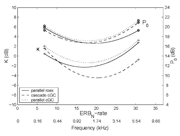
Values of the nonfilter coefficients, K and P₀, plotted as a function of center frequency on the ERB_N-rate scale for the parallel roex filter (solid line), the cascade cGC filter (dashed line), and the parallel cGC filter (dotted line). The K and P₀ functions are identified by plus and star symbols, respectively, at the ends of the lines.

The relationship between P₀ and the frequency variable, E_f, was also found to take the form of a parabola, and the parabolas for the three filter systems are shown in Fig. 5 by lines that end in stars. Once again, the parabolas for the cascade cGC, the parallel roex, and the parallel cGC filter systems are shown by dashed, solid, and dotted lines, respectively. This parameter is related to the absolute threshold and it is used to predict the way threshold asymptotes in wide-notch conditions at low stimulus levels. The functions for the three filter systems are very similar and they are also in good agreement with the P₀ estimates reported by Glasberg and Moore (2000) and Baker et al. (1998) using the incomplete roex filter.

V. SUMMARY AND CONCLUSIONS

The roex filter has been successfully used for many years to represent the magnitude response of the auditory filter in studies of tone-in-noise masking, and recently the roex(p,w,t) version, with parallel roex(p) and roex(t) filters, has been used to simulate the interaction of the “tip” and “tail” components of the cochlear filter as a function of stimulus intensity (Glasberg and Moore, 2000; Oxenham and Shera, 2003; Baker and Rosen, 2006). Nevertheless, the roex(p,w,t) filter is limited in its application because there is no time-domain version of the filter and no roex(p,w,t) filterbank to simulate basilar-membrane motion in response to complex sounds like speech and music. It is also the case that the fits provided by the complete roex(p,w,t) filter to notched-noise masking data are somewhat unstable, unless one of the high-frequency skirts is removed, in which case the magnitude response is discontinuous and the filter is physically unrealizable.

We have developed a compressive gammachirp (cGC) filter system with parallel architecture like that of the parallel roex filter and compression in the tip filter branch, to provide a filter system that has a similar magnitude response to the parallel roex filter, and which provides a basis for producing a time-domain version of the filter. Basically, we replaced the roex filters with gammachirp filters [compare Figs. 1(a) and 1(c)]. A quantitative comparison of the parallel roex and parallel cGC filters was made by fitting both to the simultaneous notched-noise masking data of Baker et al. (1998) and Glasberg and Moore (2000). The behavior of the parallel cGC filter is quite similar to that of the parallel roex filter. In particular: (1) The filters become broader as stimulus level increases at all center frequencies; (2) The filters are asymmetric with the high side sharper than the low side, and the asymmetry increases with increasing level; (3) The tails of the filters converge on both sides at high stimulus levels, indicating that the gain is effectively level independent for frequencies far removed from the center frequency; (4) The gain of the filter at its peak frequency increases as stimulus level decreases, indicating the presence of relatively strong compression; (5) The amount of compression increases with increasing center frequency, at least in the region below 2.0 kHz. It remains the case, however, that fits to notched-noise data with the parallel cGC filter are still somewhat unstable because the high-frequency skirts of the component filters interact, as with the parallel roex filter.

We also compared the fit of the cascade cGC filter (Irino and Patterson, 2001; Patterson et al., 2003) to the notched-noise data, to the fits provided by the parallel roex and parallel cGC filters. The cascade cGC filter provides at least as good a fit as either of the parallel filters to the simultaneous masking data, with 25% fewer coefficients, and the fits are stable. The advantage of the cGC filter appears to be a direct result of the architecture of the gammachirp filter with its parsimonious representation of the high-frequency side of the filter. The cascade cGC filter also provides a somewhat more precise fit to the tip of the auditory filter (as determined by the data for small notch widths) than the roex filter does. The effects of level and frequency on the cascade cGC filter system are quite similar to those described above for the parallel filter systems. Moreover, a dynamic version of the cascade cGC filter has been developed that can simulate fast-acting compression (Irino and Patterson, 2005, 2006), so the cGC filter could potentially facilitate future research on the temporal properties of auditory filtering.

In conclusion, it would appear that the compressive gammachirp filter, in either its parallel or cascade form, offers better prospects for the representation of the auditory filter than the roex filter.

References

- Allen JB. OHCs shift the excitation pattern via BM tension. In: Lewis ER, Long GR, Lyon RF, Narins PM, Steele CR, Hecht-Poinar E, editors. Diversity in Auditory Mechanics. World Scientific; Singapore: 1997. pp. 167–175. [Google Scholar]
- Allen JB, Sen D. Proceedings Computational Hearing. NATO Advanced Study Institute; Il Ciocco, Italy: 1998. A bio-mechanical model of the ear to predict auditory masking; pp. 139–162. [Google Scholar]
- Assmann PF, Summerfield Q. Modeling the perception of concurrent vowels: Vowels with different fundamental frequencies. J. Acoust. Soc. Am. 1990;88:680–697. doi: 10.1121/1.399772. [DOI] [PubMed] [Google Scholar]
- Bacon SP, Fay RR, Popper AN. Compression: From Cochlea to Cochlear Implants. Springer; New York: 2004. [Google Scholar]
- Bacon SP, Repovsch-Duffey JL, Liu L. Effects of signal delay on auditory filter shapes derived from psychophysical tuning curves and notched-noise data obtained in simultaneous masking. J. Acoust. Soc. Am. 2002;112:227–237. doi: 10.1121/1.1485972. [DOI] [PubMed] [Google Scholar]
- Baker RJ, Rosen S. Auditory filter nonlinearity across frequency using simultaneous notched-noise masking. J. Acoust. Soc. Am. 2006;119:454–462. doi: 10.1121/1.2139100. [DOI] [PubMed] [Google Scholar]
- Baker RJ, Rosen S, Darling AM. An efficient characterisation of human auditory filtering across level and frequency that is also physiologically reasonable. In: Palmer A, Rees A, Summerfield Q, Meddis R, editors. Psychophysical and Physiological Advances in Hearing: Proceedings of the 11th International Symposium on Hearing; London: Whurr; 1998. pp. 81–88. [Google Scholar]
- Carlyon RP, Datta AJ. Excitation produced by Schroeder phase complexes: Evidence for fast-acting compression in the auditory system. J. Acoust. Soc. Am. 1997;101:3636–3647. doi: 10.1121/1.418324. [DOI] [PubMed] [Google Scholar]
- Carney LH, McDuffy JM, Shekhter I. Frequency glides in the impulse responses of auditory-nerve fibers. J. Acoust. Soc. Am. 1999;105:2384–2391. doi: 10.1121/1.426843. [DOI] [PubMed] [Google Scholar]
- Cohen MA, Grossberg S, Wyse LL. A spectral network model of pitch perception. J. Acoust. Soc. Am. 1995;98:862–879. doi: 10.1121/1.413512. [DOI] [PubMed] [Google Scholar]
- Cooke MP. Modelling Auditory Processing and Organization. Cambridge University Press; Cambridge: 1993. [Google Scholar]
- Cooke M, Green P, Josifovski L, Vizinho A. Robust automatic speech recognition with missing and unreliable acoustic data. Speech Commun. 2001;34:267–285. [Google Scholar]
- de Boer E. Synthetic whole-nerve action potentials for the cat. J. Acoust. Soc. Am. 1975;58:1030–1045. doi: 10.1121/1.380762. [DOI] [PubMed] [Google Scholar]
- de Boer E, Nuttall AL. The mechanical waveform on the basilar membrane. III. Intensity effects. J. Acoust. Soc. Am. 2000;107:1497–1507. doi: 10.1121/1.428436. [DOI] [PubMed] [Google Scholar]
- Divenyi P, editor. Speech Separation by Human and Machines. Kluwer Academic; Dordrecht, The Netherlands: 2004. [Google Scholar]
- Evans EF, Pratt SR, Cooper NP. Correspondence between behavioural and physiological frequency selectivity in the guinea pig. Br. J. Audiol. 1989;23:151–152. [Google Scholar]
- Fletcher H. Auditory patterns. Rev. Mod. Phys. 1940;12:47–61. [Google Scholar]
- Glasberg BR, Moore BCJ. Derivation of auditory filter shapes from notched-noise data. Hear. Res. 1990;47:103–138. doi: 10.1016/0378-5955(90)90170-t. [DOI] [PubMed] [Google Scholar]
- Glasberg BR, Moore BCJ. Frequency selectivity as a function of level and frequency measured with uniformly exciting noise. J. Acoust. Soc. Am. 2000;108:2318–2328. doi: 10.1121/1.1315291. [DOI] [PubMed] [Google Scholar]
- Glasberg BR, Moore BCJ, Nimmo-Smith I. Comparison of auditory filter shapes derived with three different maskers. J. Acoust. Soc. Am. 1984a;75:536–544. doi: 10.1121/1.390487. [DOI] [PubMed] [Google Scholar]
- Glasberg BR, Moore BCJ, Patterson RD, Nimmo-Smith I. Dynamic range and asymmetry of the auditory filter. J. Acoust. Soc. Am. 1984b;76:419–427. doi: 10.1121/1.391584. [DOI] [PubMed] [Google Scholar]
- Goldstein JL. Modeling rapid waveform compression on the basilar membrane as multiple-bandpass-nonlinearity filtering. Hear. Res. 1990;49:39–60. doi: 10.1016/0378-5955(90)90094-6. [DOI] [PubMed] [Google Scholar]
- Goldstein JL. Relations among compression, suppression, and combination tones in mechanical responses of the basilar membrane: Data and MBPNL model. Hear. Res. 1995;89:52–68. doi: 10.1016/0378-5955(95)00121-3. [DOI] [PubMed] [Google Scholar]
- Gunawan TS, Ambikairajah E. Speech enhancement using temporal masking and fractional Bark gammatone filters. Proceedings Aust. Int. Conference on Speech Science and Technology (SST’04); Sydney. 2004. pp. 420–425. [Google Scholar]
- Hicks ML, Bacon SP. Psychophysical measures of auditory nonlinearities as a function of frequency in individuals with normal hearing. J. Acoust. Soc. Am. 1999;105:326–338. doi: 10.1121/1.424526. [DOI] [PubMed] [Google Scholar]
- Hohmann V. Frequency analysis and synthesis using a Gammatone filterbank. Acta. Acust. Acust. 2002;88:433–442. [Google Scholar]
- Houtgast T. Auditory-filter characteristics derived from direct-masking data and pulsation-threshold data with a rippled-noise masker. J. Acoust. Soc. Am. 1977;62:409–415. doi: 10.1121/1.381541. [DOI] [PubMed] [Google Scholar]
- Irino T, Patterson RD. A time-domain, level-dependent auditory filter: The gammachirp. J. Acoust. Soc. Am. 1997;101:412–419. [Google Scholar]
- Irino T, Patterson RD. A compressive gammachirp auditory filter for both physiological and psychophysical data. J. Acoust. Soc. Am. 2001;109:2008–2022. doi: 10.1121/1.1367253. [DOI] [PubMed] [Google Scholar]
- Irino T, Patterson RD. Explaining two-tone suppression and forward masking data using a compressive gammachirp auditory filterbank. J. Acoust. Soc. Am. 2005;117:2598. [Google Scholar]
- Irino T, Patterson RD. A dynamic, compressive gammachirp auditory filterbank. IEEE Trans. Audio, Speech, and Language Processing. 2006 doi: 10.1109/TASL.2006.874669. (in press) [DOI] [PMC free article] [PubMed] [Google Scholar]
- Irino T, Patterson RD, Kawahara H. Speech segregation using an auditory vocoder with event-synchronous enhancements. IEEE Trans. Audio, Speech, and Language Processing. 2006 doi: 10.1109/TASL.2006.872611. (in press) [DOI] [PMC free article] [PubMed] [Google Scholar]
- Kohlrausch A, Sander A. Phase effects in masking related to dispersion in the inner ear. II. Masking period patterns of short targets. J. Acoust. Soc. Am. 1995;97:1817–1829. doi: 10.1121/1.413097. [DOI] [PubMed] [Google Scholar]
- Kollmeier B, Holube I. Auditory filter bandwidths in binaural and monaural listening configurations. J. Acoust. Soc. Am. 1992;92:1889–1901. doi: 10.1121/1.405264. [DOI] [PubMed] [Google Scholar]
- Krumbholz K, Patterson RD, Seither-Preisler A, Lammertmann C, Lütkenhöner B. Neuromagnetic evidence for a pitch processing centre in Heschl’s gyrus. Cereb. Cortex. 2003;13:765–772. doi: 10.1093/cercor/13.7.765. [DOI] [PubMed] [Google Scholar]
- Kubin G, Kleijn WB. On speech coding in a perceptual domain. Proceedings of ICASSP99; Phoenix, AZ. 1999. pp. 2327–2330. [Google Scholar]
- Lentz JJ, Leek MR. Psychophysical estimates of cochlear phase response: Masking by harmonic complexes. J. Assoc. Res. Otolaryngol. 2001;2:408–422. doi: 10.1007/s101620010045. [DOI] [PMC free article] [PubMed] [Google Scholar]
- Lopez-Poveda EA, Plack CJ, Meddis R. Cochlear nonlinearity between 500 and 8000 Hz in listeners with normal hearing. J. Acoust. Soc. Am. 2002;113:951–960. doi: 10.1121/1.1534838. [DOI] [PubMed] [Google Scholar]
- Lutfi RA, Patterson RD. On the growth of masking asymmetry with stimulus intensity. J. Acoust. Soc. Am. 1984;76:739–745. doi: 10.1121/1.391260. [DOI] [PubMed] [Google Scholar]
- Meddis R, O’Mard LP, Lopez-Poveda EA. A computational algorithm for computing nonlinear auditory frequency selectivity. J. Acoust. Soc. Am. 2001;109:2852–2861. doi: 10.1121/1.1370357. [DOI] [PubMed] [Google Scholar]
- Moore BCJ. Cochlear Hearing Loss. Whurr; London: 1998. [Google Scholar]
- Moore BCJ. An Introduction to the Psychology of Hearing. 5th ed Academic; London: 2003. [Google Scholar]
- Moore BCJ, Glasberg BR. Auditory filter shapes derived in simultaneous and forward masking. J. Acoust. Soc. Am. 1981;69:1003–1014. doi: 10.1121/1.386950. [DOI] [PubMed] [Google Scholar]
- Moore BCJ, Glasberg BR. Suggested formulae for calculating auditory-filter bandwidths and excitation patterns. J. Acoust. Soc. Am. 1983;74:750–753. doi: 10.1121/1.389861. [DOI] [PubMed] [Google Scholar]
- Moore BCJ, Peters RW, Glasberg BR. Auditory filter shapes at low center frequencies. J. Acoust. Soc. Am. 1990;88:132–140. doi: 10.1121/1.399960. [DOI] [PubMed] [Google Scholar]
- Moore BCJ, Vickers DA, Plack CJ, Oxenham AJ. Inter-relationship between different psychoacoustic measures assumed to be related to the cochlear active mechanism. J. Acoust. Soc. Am. 1999;106:2761–2778. doi: 10.1121/1.428133. [DOI] [PubMed] [Google Scholar]
- Nelson DA, Schroder AC, Wojtczak M. A new procedure for measuring peripheral compression in normal-hearing and hearing-impaired listeners. J. Acoust. Soc. Am. 2001;110:2045–2064. doi: 10.1121/1.1404439. [DOI] [PubMed] [Google Scholar]
- Oppenheim AV, Schafer RV. Digital Signal Processing. Prentice-Hall International; London: 1975. [Google Scholar]
- Oxenham AJ, Dau T. Reconciling frequency selectivity and phase effects in masking. J. Acoust. Soc. Am. 2001a;110:1525–1538. doi: 10.1121/1.1394740. [DOI] [PubMed] [Google Scholar]
- Oxenham AJ, Dau T. Towards a measure of auditory filter phase response. J. Acoust. Soc. Am. 2001b;110:3169–3178. doi: 10.1121/1.1414706. [DOI] [PubMed] [Google Scholar]
- Oxenham AJ, Plack CJ. A behavioral measure of basilar-membrane nonlinearity in listeners with normal and impaired hearing. J. Acoust. Soc. Am. 1997;101:3666–3675. doi: 10.1121/1.418327. [DOI] [PubMed] [Google Scholar]
- Oxenham AJ, Shera CA. Estimates of human cochlear tuning at low levels using forward and simultaneous masking. J. Assoc. Res. Otolaryngol. 2003;4:541–554. doi: 10.1007/s10162-002-3058-y. [DOI] [PMC free article] [PubMed] [Google Scholar]
- Patterson RD. Auditory filter shape. J. Acoust. Soc. Am. 1974;55:802–809. doi: 10.1121/1.1914603. [DOI] [PubMed] [Google Scholar]
- Patterson RD. Auditory filter shapes derived with noise stimuli. J. Acoust. Soc. Am. 1976;59:640–654. doi: 10.1121/1.380914. [DOI] [PubMed] [Google Scholar]
- Patterson RD, Moore BCJ. Auditory filters and excitation patterns as representations of frequency resolution. In: Moore BCJ, editor. Frequency Selectivity in Hearing. Academic; London: 1986. [Google Scholar]
- Patterson RD, Nimmo-Smith I. Off-frequency listening and auditory-filter asymmetry. J. Acoust. Soc. Am. 1980;67:229–245. doi: 10.1121/1.383732. [DOI] [PubMed] [Google Scholar]
- Patterson RD, Allerhand M, Giguére C. Time-domain modeling of peripheral auditory processing: A modular architecture and a software platform. J. Acoust. Soc. Am. 1995;98:1890–1894. doi: 10.1121/1.414456. [DOI] [PubMed] [Google Scholar]
- Patterson RD, Unoki M, Irino T. Extending the domain of center frequencies for the compressive gammachirp auditory filter. J. Acoust. Soc. Am. 2003;114:1529–1542. doi: 10.1121/1.1600720. [DOI] [PubMed] [Google Scholar]
- Patterson RD, Unoki M, Irino T. Comparison of the compressive-gammachirp and double-roex auditory filters. In: Pressnitzer D, de Cheveigne A, McAdams S, Collet L, editors. Auditory Signal Processing: Physiology, Psychoacoustics, and Models. Springer; New York: 2005. [Google Scholar]
- Patterson RD, Holdsworth J, Nimmo-Smith I, Rice P. SVOS Final Report: The Auditory Filterbank. APU Report. 1987. p. 2341.
- Patterson RD, Nimmo-Smith I, Wever DL, Milroy R. The deterioration of hearing with age: Frequency selectivity, the critical ratio, the audiogram, and speech threshold. J. Acoust. Soc. Am. 1982;72:1788–1803. doi: 10.1121/1.388652. [DOI] [PubMed] [Google Scholar]
- Patterson RD, Uppenkamp S, Johnsrude I, Griffiths TD. The processing of temporal pitch and melody information in auditory cortex. Neuron. 2002;36:767–776. doi: 10.1016/s0896-6273(02)01060-7. [DOI] [PubMed] [Google Scholar]
- Patterson RD, Robinson K, Holdsworth JW, McKeown D, Zhang C, Allerhand M. Complex sounds and auditory images. In: Cazals Y, Demany L, Horner K, editors. Auditory Physiology and Perception. Pergamon; Oxford: 1992. pp. 429–446. [Google Scholar]
- Plack CJ, Oxenham AJ. Basilar-membrane nonlinearity estimated by pulsation threshold. J. Acoust. Soc. Am. 2000;107:501–507. doi: 10.1121/1.428318. [DOI] [PubMed] [Google Scholar]
- Press WH, Flannery BP, Teukolsky AA, Vetterling WT. Numerical Recipies in C. Cambridge University Press; Cambridge, UK: 1988. [Google Scholar]
- Recio A, Rich NC, Narayan SS, Ruggero MA. Basilar-membrane responses to clicks at the base of the chinchilla cochlea. J. Acoust. Soc. Am. 1998;103:1972–1989. doi: 10.1121/1.421377. [DOI] [PMC free article] [PubMed] [Google Scholar]
- Reimann HM. Invariance principles for cochlea mechanics: Hearing phases. J. Acoust. Soc. Am. 2006;119:997–1004. doi: 10.1121/1.2159428. [DOI] [PubMed] [Google Scholar]
- Robles L, Ruggero MA. Mechanics of the mammalian cochlea. Physiol. Rev. 2001;81:1305–1352. doi: 10.1152/physrev.2001.81.3.1305. [DOI] [PMC free article] [PubMed] [Google Scholar]
- Robles L, Ruggero MA, Rich NC. Basilar membrane mechanics at the base of the chinchilla cochlea. I. Input-output functions, tuning curves, and response phases. J. Acoust. Soc. Am. 1986;80:1364–1374. doi: 10.1121/1.394389. [DOI] [PubMed] [Google Scholar]
- Roman N, Wang DL, Brown GJ. Speech segregation based on sound localization. J. Acoust. Soc. Am. 2003;114:2236–2252. doi: 10.1121/1.1610463. [DOI] [PubMed] [Google Scholar]
- Rosen S, Baker RJ. Characterizing auditory filter nonlinearity. Hear. Res. 1994;73:231–243. doi: 10.1016/0378-5955(94)90239-9. [DOI] [PubMed] [Google Scholar]
- Rosen S, Baker RJ, Darling A. Auditory filter nonlinearity at 2 kHz in normal hearing listeners. J. Acoust. Soc. Am. 1998;103:2539–2550. doi: 10.1121/1.422775. [DOI] [PubMed] [Google Scholar]
- Rosengard PS, Oxenham AJ, Braida LD. Comparing different estimates of cochlear compression in listeners with normal and impaired hearing. J. Acoust. Soc. Am. 2005;117:3028–3041. doi: 10.1121/1.1883367. [DOI] [PMC free article] [PubMed] [Google Scholar]
- Unoki M, Akagi M. A method of signal extraction from noisy signal based on auditory scene analysis. Speech Commun. 1999;27:261–279. [Google Scholar]
- Unoki M, Tan CT. Estimates of auditory filter shape using simultaneous and forward notched-noise masking. Proceedings of Forum Acusticum 2005; Budapest, Hungary. 2005. pp. 1497–1502. [Google Scholar]