Fast methods for spatially correlated multilevel functional data

Abstract

We propose a new methodological framework for the analysis of hierarchical functional data when the functions at the lowest level of the hierarchy are correlated. For small data sets, our methodology leads to a computational algorithm that is orders of magnitude more efficient than its closest competitor (seconds versus hours). For large data sets, our algorithm remains fast and has no current competitors. Thus, in contrast to published methods, we can now conduct routine simulations, leave-one-out analyses, and nonparametric bootstrap sampling. Our methods are inspired by and applied to data obtained from a state-of-the-art colon carcinogenesis scientific experiment. However, our models are general and will be relevant to many new data sets where the object of inference are functions or images that remain dependent even after conditioning on the subject on which they are measured. Supplementary materials are available at Biostatistics online.

1. INTRODUCTION

We propose fast, principal component-based methods for the analysis of hierarchical functional data when the functions at the lowest level of the hierarchy are correlated. The methodology provides an intuitive and natural decomposition of observed functional variability, can be extended to larger and more complex data structures, and is more computationally efficient than competing methods. Our methods are motivated by and applied to data obtained from a state-of-the-art colon carcinogenesis scientific experiment. However, our models are general and will be relevant to many new data sets where the object of inference are functions or images that remain dependent even after conditioning on the subject on which they are measured.

Our basic framework is developed for multilevel data structures of the following type: (1) groups, (2) subjects within groups, (3) units within subjects, and (4) subunits. This setup is inspired by analysis of variance (ANOVA) structures with 2 important differences. First, the measurements at the unit level are functions evaluated at subunits and thus the subunits are not treated as a separate level. Second, conditional on the subjects, the unit measurements may be spatially correlated. The aim of our methodology is to provide a computationally efficient methodology with the following goals: (1) to provide inference on the group mean differences; (2) to quantify the spatial covariance between functional unit responses and hence to provide an understanding of how the units influence/predict one another; (3) to provide a decomposition of the observed functional variability into within- and between-unit and measurement error variability; (4) to suggest simpler parametric models where simplifications are warranted by the data; and (5) to allow sensitivity analyses such as the deletion of single subjects or groups of subjects.

There are many instances of data that have the structure we discuss or a structure closely related to it. Here we mention a few; the key point being that each subject has a set of units, which are in fact measurements of functions and which, given the subject, are spatially correlated. The first example is data generated from a study of brain activity using quasi-continuous electroencephalographic (EEG) signals. In this study, subjects wear a helmet that records tens of EEGs from various parts of the brain for up to 48 h. In this case, units are individual EEG signals, which have a natural spatial correlation because they are collected from the same brain. The second example is gene expression data (Xiao and others, 2009). In this case, the groups are individuals, the subjects are chromosomes, and the units are genes. When gene expression is measured over time, we have spatially correlated functions within a subject since the expression levels of genes on the same chromosome frequently exhibit significant spatial correlationÓ (see Xiao and others, 2009). The third example concerns data obtained from studies of calcium ion cellular levels (Martinez and others, 2010). In this case, the subjects are individuals and the units are cells. Time-course calcium ion signals are measured for each cell producing a time series for each cell. As the location of each cell is known, it is reasonable to assume and study the spatial correlation of these time series. The last example concerns data from a colon carcinogenesis study. In this case, the groups are groups of rats who are fed the same diet before a carcinogen exposure, the subjects are rats, and the units are colonic crypts. The concentration of p27 (Sgambato and others, 2000), a cell cycle inhibitor protein, is measured for each cell in the crypt, as a function of the relative cell positions within the crypt (Grambsch and others, 1995; Roncucci and others, 2000). Within each rat the functional response of the crypt the p27 expression exhibits spatial correlation. For more details see Section 6.

We now introduce our model. Throughout the paper, the symbol Δ will refer to spatial locations or lags. Denote by Y_dri(t,Δ_dri) the measured response at the subunit location t within the unit i = 1,…,M_dr located at the spatial location Δ_dri within the subject r = 1,…,R_d from group d = 1,…,D. Our model for Y_dri(t,Δ_dri) is Y_dri(t,Δ_dri) = μ_d(t) + Z_dr(t) + 𝒬_dri(t,Δ_dri) + ϵ_dri(t), where μ_d(·) is the group mean function and Z_dr(·) is the subject-specific deviation from the group mean. The second level unit-specific deviation from the subject-specific mean is, for a unit at spatial location Δ_dri, 𝒬_dri(t,Δ_dri), and ϵ_dri(t) is noise. We note in passing that neither the group-level mean, μ_d(t), nor the subject-level mean, μ_d(t) + Z_dr(t), is indexed by the spatial locations Δ of the units within the subjects, which is because neither the groups nor the subjects have spatial locations.

By incorporating the spatial location Δ_dri of the units within the subjects, we are specifically allowing for the possibility that these units are spatially correlated given the subject. As a means of modeling this spatial correlation, we decompose 𝒬_dri(t,Δ_dri) into 2 parts, one that does not exhibit spatial correlation and one that does. We write 𝒬_dri(t,Δ_dri) = W_dri(t) + U_dr(Δ_dri), where W_dri(t) depends only on the subunit location within the unit, t, and U_dr(Δ_dri) depends only on the unit spatial location, Δ_dri. The correlation between the unit mean functions, 𝒬_dri(t,Δ_dri), is modeled explicitly via the random spatial process U_dr(Δ_dri). This is a standard technique in multilevel modeling that we adopt in our more complex multilevel functional framework. We assume that Z_dr(t), W_dri(t), U_dr(Δ_dri), and ϵ_dri(t) are zero mean, mutually uncorrelated random processes and that ϵ_dri(t) is a white noise process. In Section 3, we present more details about this model and its assumptions.

2. METHODS TO MODEL FUNCTIONAL DATA

The analysis of functional data is an area of modern statistics under intense methodological development; see, for example, the excellent monograph by Ramsay and Silverman (2005). There already exists a rich literature dedicated to the analysis of single-level functional data (Shi and others, 1996; Brumback and Rice, 1998; Staniswallis and Lee, 1998; Wang, 1998; Fan and Zhang, 2000; Rice and Wu, 2001; Wu and Zhang, 2002; Liang and others, 2003; Wu and Liang, 2004; Wu and Zhang, 2006). Grambsch and others (1995) employed functional data analysis-based methods for the first time to model the crypt data structure similar to the one we consider here, although they assumed only one level of hierarchy.

In a multilevel functional framework, Guo (2002) proposed a spline-based approach for functional mixed-effects models. Morris and others (2001) analyzed hierarchical models with a structure similar to ours based on DNA adduct data, using frequentist methods, but they had no available spatial measurements of the crypt positions. Di and others (2009) introduced multilevel functional principal component analysis (FPCA) in the context of sleep studies. Their framework is the functional equivalent of multi-way ANOVA, uses functional principal component (FPC) bases to reduce dimensionality and accelerate algorithms, and assumes independence of functions at the lowest level of the hierarchy. Morris and others (2003) and Morris and Carroll (2006) developed a wavelet-based methodology for modeling functional data occurring within a nested hierarchy. However, Morris and others (2003) assumed that the functions at the lowest level of the hierarchy (crypts) are independent. Morris and Carroll (2006) allow for general covariance structures but their approach is not tailored to spatial dependence of the type arising in our data.

There have been previous analyses of data with correlation of the functions at the deepest level of the hierarchy. Baladandayuthapani and others (2008) developed a Bayesian methodology for a data structure exactly as ours. However, there are key differences. First, we use multilevel principal components, while Baladandayuthapani and others used regression splines. Second, we use a method of moments approach combined with best linear unbiased prediction (BLUP), while Baladandayuthapani and others used Bayesian analysis. These 2 differences make our approach much faster, as detailed in Section 5.2. As a consequence, we are now able to conduct routine and large simulation studies as well as quickly analyze previously unexplored facets of the data. Third, our methods can easily be applied to data sets that are orders of magnitude larger than the data set considered in this paper.

A key technical difference with Baladandayuthapani and others (2008) is how the functions at the deepest level of the hierarchy, the units, are modeled. In our model, we decompose the functions at the unit level, 𝒬_dri(t,Δ_dri), additively, involving 2 uncorrelated components: a random function W_dri(t) and a spatial process U_dr(Δ_dri). In contrast, Baladandayuthapani and others model 𝒬_dri(t,Δ_dri) via regression splines with spatially correlated random coefficients, β_dri. Stacking the coefficients into a vector ℬ_dr, they assume that the coefficients have a separable covariance structure, cov(ℬ_dr) = Σ_dr(Δ)⊗Σ₁, where Σ_dr(Δ) is a spatial correlation matrix and Σ₁ = cov(β_dri) which, in order to achieve parsimony, is forced to have the same form as the mixed-model approach to smoothing (Ruppert and others, 2003).

Li and others (2007) took a nonparametric approach to this problem using kernel smoothing. A key difference between our methods and theirs is that they treat the sampling subjects, the rats, as fixed and not random; thus removing one level of the hierarchy. Their key aim is to estimate the correlation function between the units, and they too take a separable structure approach, so that, conditional on the subject, the covariance between a measurement in a unit at subunit s and a measurement at subunit t of a second unit distance Δ from the first is modeled as G(s,t)ρ(Δ), whereas ours is modeled simply as ρ(Δ)σ_u²: of course, within a single unit, the covariance is K^W(s,t) + ρ(Δ)σ_u². A major advantage of our approach is that it easily scales up: we can handle more realistic situations where many subjects have only a few units. In contrast, the approach of Li and others assumes that there is a fixed number of subunits per unit, and that there are sufficient units to ensure that the subject-specific function is accurately estimated.

The paper is organized as follows. Section 3 introduces our statistical framework and model assumptions for spatially correlated multilevel functional data. Section 4 presents estimation methods for each model component. Section 5 outlines the main results of the simulation study performed. Section 6 presents our inferential results for the colon carcinogenesis data, and Section 7 provides the concluding remarks. To ensure reproducibility of our results accompanying software, simulations, and analyses results described in this paper are available as supplementary at Biostatistics online.

3. MODEL

3.1. Basic model and general setup

In this section, we provide the details of the modeling approach. The decomposition described in Section 1 leads to our basic model:

(3.1)

where μ_d(·) is the group mean fixed effect, Z_dr(·) and W_dri(·) are random functions at the subject and unit level, respectively, U_dr(·) is a spatial process, and ϵ_dri(t) is white noise. We use the framework suggested by Di and others (2009) to model Z_dr(t) and W_dri(t), the level 1 and 2 processes, respectively. If Z_dr(t) and W_dri(t) are processes in L²[0,1] and {ϕ_k⁽¹⁾(t):k ≥ 1} and {ϕ_ℓ⁽²⁾(t):ℓ ≥ 1} are 2 orthonormal bases in L²[0,1], that is ∫₀¹ϕ_k⁽¹⁾(t)ϕ_k′⁽¹⁾(t)dt = δ_kk′, where δ_kk′ is the Kronecker delta, then Z_dr(t) and W_dri(t) have unique representations Z_dr(t) = ∑_{k = 1}^∞ξ_dr,kϕ_k⁽¹⁾(t) and W_dri(t) = ∑_{l = 1}^∞ζ_dri,ℓϕ_l⁽²⁾(t), where the random coefficients ξ_dr,k and ζ_dri,ℓ are given by ξ_dr,k = ∫Z_dr(t)ϕ_k⁽¹⁾(t)dt and ζ_dri,ℓ = ∫W_dri(t)ϕ_l⁽²⁾(t)dt, respectively. Thus, model (3.1) becomes

(3.2)

where t∈[0,1] is an arbitrary subunit within the ith unit and Δ_dri is the spatial location of this unit within subject r. This form of the model cannot be used in practice because of the infinite summation, and the following truncated version will be used instead

(3.3)

where K₁ and K₂ are truncation lags defining a double sequence of approximating models for the infinite-dimensional model (3.2). Section 4.6 provides our procedures for selecting a reasonable number of orthonormal eigenvectors at both levels. In Section 4, we will also describe how we construct and estimate the basis functions.

While model (3.3) may look complex and its implementation may seem difficult, we will show that model inference involves a sequence of simple steps that results in fast implementation; in R the model can be fit in seconds. We will use parsimonious decompositions of the first and second level functional spaces using principal components as in Di and others (2009). This will ultimately ensure important computational advantages over previous methods. In contrast to Di and others, our approach allows for correlation among functions at the lowest level of the hierarchy 𝒬_dri(t,Δ_dri). This correlation is allowed to vary with the distance between the location of the units and is of considerable scientific interest in our application.

We make the following 3 assumptions:

• A.1 E(ξ_dr,k) = 0, E(ξ_dr,k²) = λ_k⁽¹⁾, E(ξ_dr,kξ_dr,k′) = 0 for k ≠ k′;

• A.2 E(ζ_dri,ℓ) = 0, E(ζ_dri,ℓ²) = λ_l⁽²⁾, E(ζ_dri,ℓζ_dri,ℓ′) = 0 for l ≠ ℓ′;

• A.3 {ξ_dr,k:k = 1,2,…} are uncorrelated with {ζ_dri,ℓ:l = 1,2,…}.

Assumptions A.1 and A.2 are standard in functional models, while A.3 corresponds to our assumption that Z_dr(·) and W_dri(·) are uncorrelated. The functional bases {ϕ_k⁽¹⁾(t):k = 1,2,…} and {ϕ_l⁽²⁾(t):l = 1,2,…} at levels 1 and 2 of the hierarchy, respectively, are each assumed to be orthonormal but are not required to be mutually orthonormal.

We also assume that {U_dr(Δ):Δ∈R} is a zero-mean, second-order stationary, isotropic random process (Cressie, 1991, Chapter 2) in L²(R), observed at locations Δ_dr1,…,Δ_drMdr in [0,L]; this means that the process has constant variance σ_U², and its correlation function depends only on the distance between the sampling locations. In addition, if ρ(Δ) = corr{U_dr(Δ^*),U_dr(Δ^* + Δ)} denotes the process correlation function, we assume

• A.4 limρ(Δ) = 0 as the distance lag Δ → ∞;

• A.5 limρ(Δ) = 1 as the distance lag Δ→0.

Estimating the correlation of this underlying spatial process plays a major role in our paper.

3.2. Further model specification

In theory, the choice of bases in Section 3.1 is not important. For example, in the same application Baladandayuthapani and others (2008) use regression splines, while Morris and Carroll (2006) use wavelets. We use parsimonious orthonormal bases at both levels of the hierarchy, estimated from the data, to obtain fast and robust computational algorithms; see Section 5 for more information about computation times.

Our multilevel FPCA (MFPCA) is based on the covariance operators K^Z(t,s) = cov{Z_dr(t),Z_dr(s)} of the Z_dr(·) process and K^W(t,s) = cov{W_dri(t),W_dri(s)} of the W_dri(·) process. Mercer's theorem provides the spectral decomposition of K^Z(s,t) = ∑_{k = 1}^∞λ_k⁽¹⁾ϕ_k⁽¹⁾(s)ϕ_k⁽¹⁾(t) and K^W(s,t) = ∑_{ℓ = 1}^∞λ_ℓ⁽²⁾ϕ_ℓ⁽²⁾(s)ϕ_k⁽²⁾(t), where λ₁⁽¹⁾ ≥ λ₂⁽¹⁾ ≥ … and λ₁⁽²⁾ ≥ λ₂⁽²⁾ ≥ … are the ordered level 1 and level 2 eigenvalues and {ϕ_k⁽¹⁾(t)}_k and {ϕ_ℓ⁽²⁾(t)}_ℓ are the corresponding eigenfunctions. To use the Karhunen–Loève expansions of Z_dr(t) and W_dri(t) one needs to obtain asymptotically consistent estimators of the covariance operators K^Z and K^W. We now provide such estimators based on the method of moments and on the decomposition of the total covariance operator.

Denote by K_T^Y(t,s) = cov{Y_dri(t,Δ_dri),Y_dri(s,Δ_dri)} the total covariance of the observed process Y_dri(·,Δ_dri), by K_B^Y(t,s,Δ) = cov{Y_dri(t,Δ_dri),Y_drj(s,Δ_drj)} the between-unit covariance, and by the within-unit covariance at subunit locations (t, s) for units situated at distance Δ = |Δ_dri − Δ_drj|. Then,

(3.4)

where δ_ts is equal to 1 when t = s and 0 otherwise. Moreover,

(3.5)

(3.6)

where ν(Δ) = cov{U_dr(Δ + Δ^*),U_dr(Δ^*)} = σ_U²ρ(Δ) is the covariance function at lag Δ of the process U_dr. Section 4 provides the technical details for model estimation based on the total covariance operator decomposition introduced in this section.

4. MODEL ESTIMATION

4.1. Overview

Equations (3.4–3.6) provide the intuition behind the road map for our estimation procedure. The steps of the algorithm are the following: 1)

1. Obtain an estimator of the covariogram ν(Δ), see Section 4.2; 2)

2. Use (3.4–3.6) to estimate K^Z(t,s) and K^W(t,s) and then estimate the eigenvalues and eigenfunctions of the K^Z(t,s) and K^W(t,s) operators, see Section 4.3; 3)

3. Obtain estimates of the group-specific mean functions μ_d(t), see Section 4.4; 4)

4. Estimate the principal component scores, see Section 4.5; 5)

5. Use (3.6) for t = s to estimate σ_ϵ², see Section 4.7.

The remaining sections provide details for each individual step of this procedure.

4.2. Spatial covariance

The covariance function of the spatial process ν(Δ) quantifies the relationship between observations located within units at distance Δ apart. We propose a method of moments estimator for the covariance function ν(Δ). Because of the complex structure of model (3.3), estimation of the spatial covariance function entails a preliminary estimation of the within-units covariance function K_W^Y(·,·,Δ). Let be an estimator of the within-units covariance functions K_W^Y(t,s,Δ) at subunit locations (t,s) for units situated at distance Δ apart, defined as follows. Fix k and define the weights w_drij(Δ) = w_drij^(k)(Δ) = 1{|Δ_dr,ij|∈𝒩_k(Δ)}, where 𝒩_k(Δ) is the subset of kth closest values to Δ among all the pairwise unit distances and Δ_dr,ij = |Δ_dri − Δ_drj|. Then estimate

(4.1)

by averaging the products of pairwise differences of responses at the subunit locations (t, s) and within units located at distances that are among the kth closest values to Δ. Equation (4.1) can be viewed as a kernel estimator with moving kernel bandwidth, and thus it provides a consistent estimator of K_W^Y(t,s,Δ).

Using (3.6) along with the Assumption A.4 that the correlation function vanishes beyond a certain range, we modify this estimator as follows. Let Δ^* be a preset threshold such that ρ(Δ) is negligible beyond Δ^*; the range [0,Δ^*] is typically referred to as the covariance range (see Cressie 1991, Chapter 2.3). To correct for the decay of the spatial correlation, we define _W^Y(t, s, Δ) as

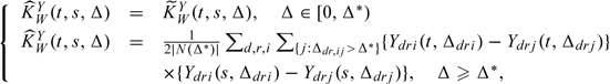(4.2)

where |N(Δ^*)| is the cardinality of the set N(Δ^*) = {(d,r,i,j):Δ_dr,ij > Δ^*}. Using _W^Y(t, s, Δ), we define an estimator for the spatial covariance function ν(Δ) by

(4.3)

where Δ∈[0,Δ^*]. This is a consistent estimator of the covariance function ν(Δ) because (a) (Δ) is based on the difference between 2 consistent estimators of K_W^Y(t,s,Δ) and K_W^Y(t,s,Δ^*) for which K_W^Y(t,s,Δ^*) − K_W^Y(t,s,Δ) = ν(Δ) − ν(Δ^*) and (b) the correlation function, ρ(Δ), is assumed to satisfy Assumption A.4, and hence ν(Δ^*)≈0. The covariance estimator is nonsmooth, a feature inherited from .

An important advantage of estimating the covariance function ν(Δ) via the cross-semivariogram K_W^Y(t,s,Δ) is that the resulting estimator does not depend on the estimation of the group mean functions. This was achieved by taking pairwise differences within the same group (see (4.1)). Estimating the covariance through the cross-covariogram of the process has been considered by Li and others (2007), who suggest a kernel estimator with a suitably selected global bandwidth. Another alternative, perhaps closer to our approach, is to use quantile binning, where the range of the spatial process is partitioned in bins determined by equally spaced quantiles of the unit distances data. Regardless of the method used (k-nearest neighbor, quantile binning, or kernel smoothing), the smoothing parameter can either be fixed to a reasonable value or can be estimated using standard methods such as cross-validation.

4.3. Covariance operators

The next step is to estimate the covariance operators at levels 1 and 2, K^Z and K^W. For this, we use the threshold Δ^* defined in Section 4.2 as the value of Δ for which the observations corresponding to units situated at distance equal to or larger than this lag are assumed uncorrelated. Equations (3.4–3.6) along with the Assumptions A.4 and A.5 suggest a natural estimator for the covariance operator at each level. To begin with, let _T^Y(t, s) be the method of moment estimator of the total covariance of the observed process: , where . The estimator of K^Z(t,s) is defined as

where |N(Δ^*)| is the cardinality of the set N(Δ^*) = {(d,r,i,j):Δ_dr,ij > Δ^*}. The estimator of K^W(t,s) is defined by

(4.4)

for t ≠ s, where is an estimator of the process variance U. The diagonal terms t = s are left out in the estimation of ^W(t,s), in order to eliminate the nugget effect, implied by expression (3.6). For t = s, we define ^W(t, s) by predicting K^W(t,t) using a bivariate thin-plate spline smoother of ^W(s,t), s ≠ t, a method proposed by Di and others (2009) and based on the original “smoothing on the diagonal” ideas described by Yao and others (2003) and Yao and Lee (2006) for single-level FPCA.

Once consistent estimators of K^Z(t,s) and K^W(t,s) are available, the spectral decomposition and functional regression proceed as in the classical single-level functional case. Thus, eigenanalysis for each ^Z(t,s) and ^W(t,s) provides consistent estimates of the eigenvalues _k⁽¹⁾, _ℓ⁽²⁾ and eigenfunctions _k⁽¹⁾, _ℓ⁽²⁾. The estimators ^Z(t, s) and ^W(t,s) may not be positive definite; in this paper we use trimming the eigenvalue–eigenfunctions pairs where the eigenvalues are negative (Hall and others, 2008; Müller, 2005; Yao and others 2005). Hall and others (2008) shows that this method is more accurate than the method of moments.

Remarks on theoretical properties.

Because the estimators (Δ), ^Z, and ^W are method of moments estimators, it is relatively straightforward to establish their consistency and asymptotic normality. We only provide the less well-known results and the intuition behind the proofs.

Consider first the spatial covariance estimator (Δ). This estimator is based on 2 estimators _W^Y(t, s, Δ) and _W^Y(t, s, Δ^*). The cross-semivariogram estimator, _W^Y(t, s, Δ), is a standard extension of the classical method of moments estimator of the semivariogram due to Matheron (1962) to address the case of irregularly spaced data, which replaces a fixed lag Δ by a “tolerance” region around Δ. The set 𝒩_k(Δ), used in (4.1), is precisely the tolerance region around Δ that contains k distinct pairs, with k ≥ 30 (see Journel and Hujibregts, 1978) and is assumed to be as small as possible to retain the spatial resolution. For fixed subunits (t, s), the asymptotic Gaussian distribution of such extended estimators of the sample cross-semivariogram, and hence their consistency, has been established under appropriate mixing conditions, which ensure that the process dies off sufficiently quickly as the lag distance Δ increases (see Cressie,1991, Chapter 2.4, and the references therein). The properties of the cross-semivariogram _W^Y(t,s, Δ^*) are determined in a similar way, with the difference that the tolerance region around Δ^* contains all the pairs at distance greater than Δ^*. Under the assumption that the spatial covariance is assumed to be negligible beyond the preset threshold Δ^*, it follows that the estimator _W^Y(t, s, Δ^*) is asymptotically consistent as well. This concludes our intuitive justification about the consistency of (Δ).

Consider now the functional covariance operators ^Z and ^W. Note that the previous arguments also imply that the covariance operator ^W is asymptotically consistent. To show that ^Z is consistent, it is sufficient to show that the estimator _T^Y is consistent. This is straightforward because _T^Y is simply a method of moment estimator of the total covariance and thus standard asymptotic theory applies.

4.4. Group specific mean functions

An important characteristic of the covariance estimators obtained in Sections 4.2 and 4.3 is that they do not depend on the group mean functions. Thus, estimating the group mean functions can be viewed as a regression problem with known (or estimated) residual covariance. In the parametric case, this problem can be reduced to weighted least squares error regression. In the nonparametric case, standard smoothing techniques, such as penalized splines, could be applied to reweighted (or pre-whitened) data. Alternatively, the penalized likelihood criterion can be adapted to incorporate a known covariance structure of the residuals. We use the generalized (weighted) least squares approach and estimate the group mean functions _d(t) under the parametric assumption that the functions have a linear form in Section 5 and a quadratic form in Section 6.

4.5. Principal component scores

Assume for now that the truncation lags K₁, K₂, and the eigenfunctions, ϕ_k⁽¹⁾(·), ϕ_l⁽²⁾(·) are estimated and fixed; the selection of K₁ = K₁(n) and K₂ = K₂(n), where n = ∑_{d = 1}^DR_d is the total number of subjects will be discussed in Section 4.6. We propose to estimate the FPC scores {ξ_dr,k}_{k = 1}^K₁ and {ζ_dri,ℓ}_{l = 1}^K₂ using BLUP. For simplicity of notation, denote by Y_dri(t,Δ_dri), the new response obtained after subtracting the group mean function estimates, Y_dri(t, Δ_dri) − _d(t). Let 𝕐_dr be the vector obtained by stacking the responses Y_dri(t,Δ_dri) first over t and then over i, which has the covariance matrix Σ_dr. If B_dr^T = (Φ_dr1^(1)T,…,Φ_drMdr^(1)T) denotes the ∑_{i = 1}^M_drN_dri×K₁ matrix with elements {ϕ₁⁽¹⁾(t),…,ϕ_K1⁽¹⁾(t)}, where the arguments for t match those of the corresponding row of 𝕐_dr and 𝔹_dr = diag(Φ_dr1⁽²⁾,…,Φ_drMdr⁽²⁾) denotes the ∑_{i = 1}^M_drN_dri×K₂M_dr matrix of ϕ_l⁽²⁾(t)‘s, then

(4.5)

where Σ_ξ = diag(λ₁⁽¹⁾,…,λ_K1⁽¹⁾), Σ_β = diag(λ₁⁽²⁾,…,λ_K2⁽²⁾), Σ_ζ = I⊗Σ_β, and Σ_U,dr is the M_dr×M_dr variance covariance matrix of the M_dr×1 vector of {U(Δ_dri):i = 1,…,M_dr}. Here 1_dri denotes the N_dri×1 vector of ones and 𝔼_dr = diag(1_dr1,…,1_drMdr). The matrix Σ_dr is of size ∑_{i = 1}^M_drN_dri, where N_dri is the number of subunit locations within unit i. The BLUP calculations require inverting the matrix Σ_dr or _dr, which are square matrices of size equal to the total number of subunit locations within a subject, ∑_{i = 1}^M_drN_dri. We avoid this problem by using a computational trick that allows us to invert matrices of size at most equal to the number of units within a subject, M_dr; see Appendix A.1 in the supplementary material available at Biostatistics online for details. Thus, our methods do not depend essentially on the size and complexity of the functions at the unit level and can handle a very large number of units.

4.6. The number of eigenfunctions and eigenvalues

For simplicity, we consider the case when there are the same number of subunit locations N in each unit and the same number of units M for each subject. Modifications for a variable number of units and subunits are simple although notationally tedious.

Di and others (2009) proposed to use the percent explained variance to estimate the number of eigenfunctions that provide a good approximation to the infinite-dimensional processes {Z_dr(·)} and {W_dri(·)}. More precisely, let P₁ and P₂ be 2 thresholds and choose K₁ as

This criterion is intuitive, easy to explain to scientific collaborators, and trivial to compute. A disadvantage is that the thresholds P₁ and P₂ need to be chosen. We recommend doing this via simulations, which can be quickly conducted using our methods.

Alternatively, one can use likelihood ratio testing. Let _dr be the M-dimensional vector of the predicted values of the collection {U_dr(Δ_dri):Δ_dri}. For a choice K₁ and K₂, we denote by the K₁-dimensional vector of the estimated FPC scores at level 1 of the hierarchy, by the MK₂-dimensional vector of the estimated FPC scores at level 2. Furthermore, let 1^M be the M-dimensional vector of ones, let , let (1) be the N×K₁ matrix of estimated eigenfunctions _k⁽¹⁾(t), and let is the MN×MK₂ matrix of estimated eigenfunctions _l⁽²⁾(t), where I_M is the identity M × M matrix. Let 1_N be the N × 1 vector of ones and 𝔼 = I_M⊗1_N. Define by ℓ(K₁,K₂) a pseudo-Gaussian log-likelihood for the observed sample, conditional both on the estimated FPC scores and and on the predicted values of _dr‘s which, except for irrelevant constants, is given by

(4.6)

where Σ_dr is the covariance matrix of the vector 𝕐_dr obtained by stacking Y_dri(t,Δ_dri). This matrix is of size NM = 600 in our application. In the Appendix A.2 of the supplementary material available at Biostatistics online, we show how to compute the determinant of _dr by using only determinants of matrices of much smaller dimension.

Because of the hierarchy of the eigenvalues λ₁^(l) ≥ λ₂^(l) ≥ … for l = 1, 2, it is necessary to define the likelihood ratio test (LRT) only for nested models. We define the LRT for testing (K₁,K₂) versus (K₁ + δ,K₂ + 1 − δ) by 2ℓ(K₁ + δ,K₂ + 1 − δ) − 2ℓ(K₁,K₂), where δ = 0, 1. Both δ = 0 and δ = 1 correspond to testing the null hypothesis that a variance component is equal to zero in a linear mixed-effects model. The asymptotic null distribution of the LRT is a 50–50 mixture of 0.0 and a χ₁² (Stram and Lee, 1994), whose 0.95 quantile is 2.71. When the number of independent observations is not large enough one can refine the finite sample approximation of the LRT using methods described in Crainiceanu (2008) and Greven and others (2008) based on the results of Crainiceanu and Ruppert (2004) and Crainiceanu and others (2005).

We propose to use a sequence of LRTs with α-level equal to 0.05. This is equivalent to minimizing an information criterion IC(K₁,K₂) = − 2ℓ(K₁,K₂) + Q(K₁ + K₂), where Q = 2.71. A popular alternative to this criterion is the Akaike information criterion (AIC) (Müller and Stadtmüller, 2005), which uses Q = 2 and is equivalent to sequential LRT with an α-level of 0.079.

4.7. Measurement error variance

Finally, using (3.6), we estimate the variance of the measurement error by

(4.7)

where ^W(t,t) is defined by expression (4.4) for t = s. Alternatively, one can use (3.4). The estimated values for the variance of the measurement error are roughly the same in our experience. We use (3.6) to estimate σ_ϵ² for the simulation studies and our data analysis.

5. SIMULATION STUDIES

5.1. Outline of the main results

We conducted a simulation study to assess the performance of the proposed estimation procedure in realistic settings. The details of the study and of the results are presented in Appendix B of the supplementary material available at Biostatistics online. In this section, we summarize the main findings based on 1000 generated data sets and discuss the algorithm performance.

In short, we generate data from model (3.2) under 6 scenarios given by 2 different spatial designs of the unit locations and 3 types of spatial autocorrelation functions, which differ not only in the range they decay to zero but also in their monotonicity and behavior at Δ = 0. Figure 1 gives the mean of the adjusted correlation estimators along with their 90% pointwise confidence intervals. Here (Δ) is the k-nearest neighbor estimator of ν(Δ) adjusted for positive semi-definiteness (Christakos, 1984). The correlation estimators are very nearly unbiased and suggest somewhat smaller variability in the case of uniform design than in the actual design of the colon carcinogenesis study of unit locations. Our methodology performs remarkably well at recovering the true eigenfunctions and at correctly identifying the different levels of variation. These results and many other results presented in the supplementary material available at Biostatistics online confirm the well behavior of the estimators of all the model components.

Fig. 1.

The mean of the estimated correlation functions along with their pointwise 90% confidence interval in the case of the uniform design (top panel) and the colon carcinogenesis study design (bottom panel) of the units location. The true correlation functions (grey line) are ρ₁ (left), ρ₂ (middle), and ρ₃ (right); the estimates are by k-nearest neighbor with positive semi-definite adjustment (solid lines).

5.2. Comparative algorithm performance

As mentioned in the introduction, our method is far more computationally efficient than that of its closest competitor, the one introduced by Baladandayuthapani and others (2008). On a test data set with D = 2, R = 6, M_dr = 20 and N_dri = 30, our R-implementation takes 5 s on a 8-core Pentium processor with 32 GB of RAM, while theirs takes over 5 h. This difference allowed us to perform the simulation analyses described in this section. Also, we can perform analyses that would be computationally daunting for the methods in Baladandayuthapani and others (2008). For example, in Section 6, we present a cross-validation analysis of the colon carcinogenesis data by deleting one rat at a time. More importantly, our methods can easily be extended to 50 or 500 rats, whereas it is reasonable to assume that the algorithm of Baladandayuthapani and others would be significantly slower in these cases.

6. DATA ANALYSIS

We now apply our proposed method to the colon carcinogenesis study. A detailed description of the study was previously published in Baladandayuthapani and others (2008). Briefly, the aims of the study were to analyze the association between diet (fish/corn) and colon cancer and to understand the mechanisms underlying the genesis of the colon cancer. We focus on the data from the rats assayed at 24 h after the carcinogen exposure. These data contain a total of 12 rats divided into 4 diet groups: corn or fish oil with or without butyrate supplement. For each rat, the response variable p27 is measured for all cells within several colonic crypts situated at various locations across the colon tissue. There are about 20 crypts per rat and 18–37 cells per crypt with an average of 26.6 cells per crypt. Data are log-transformed before the start of the analysis. Figure 2 shows the log p27 along the crypt for the first 3 crypts within 2 rats. The circles represent pairs {t, log p27 (t)}, where t is the relative cell position and the solid lines represent the estimated mean function using penalized splines. The goals of the analysis are (1) to estimate the diet group mean functions of the p27 expression level, (2) to estimate the spatial correlation of the crypt mean functions, and (3) to quantify the various levels of uncertainty, namely rats, crypts, and spatial. To address these goals, we use the methodology outlined in Section 4.

Fig. 2.

Expression level of p27 along the crypt for the first 3 crypts within 2 rats.

6.1. The correlation between crypt mean functions

The first step is to estimate the spatial correlation between the crypt mean functions. Figure 3 shows the k-nearest neighbor estimate of the correlation as a function of the crypt location distance Δ. The cutoff Δ^* is chosen to reflect the best scientific knowledge and should not depend on the specific subjects nor on the number of subjects in the study. We used a cutoff value of Δ^* = 1000 microns because the biologists do not expect the expression level of p27 measured within crypts that are more than 1000 microns apart to be correlated. We used k-nearest neighbor method with k = 111 estimated by cross-validation. This specific value of the neighboring size k corresponds to crypt distances ranging between 90 and 300 microns, with larger distances for larger Δ.

Fig. 3.

The estimated correlation function (left panel) with positive semi-definiteness adjustment (solid line) or without (dashed line). Estimates of the correlation function by taking one rat out (dashed line) for all the rats in the colon carcinogenesis study

The left panel displays the correlation estimator for the entire data set. The correlation pattern is interesting, indicating a relatively sharp decline corresponding to crypts distances of up to 100 microns, followed by a moderate decline for crypts that are between 100 and 500 microns apart and then a very steep decay for crypts that are between 500 to 600 microns apart. Correlation is small negligible for distances between crypts larger than 600 microns.

The right panel of Figure 3 displays the estimates of the correlation obtained by leave-one-rat-out in the analysis. For the sensitivity analysis, the neighboring size was adjusted for each case separately. The results suggest some sensitivity to individual rats. When removing rats from the analysis, the correlation function can vary by up to 0.30, especially for crypt locations that are over 100 microns apart. This type of analysis would have been computationally prohibitive for competing methods but is routine using our approach.

6.2. Rat/Crypt/Spatial level variability

The second step is to quantify the spatial variability as well as the variability corresponding to the rat level and the crypt level. Our approach estimated the crypts spatial variability _U² to 4.88 at a scale of 10⁻³. To estimate the uncertainty at both the rat and crypt levels, we need first to select the number of components at each level: we use the LRT, AIC and the percent variance explained criteria described in Section 4.6. The percent variance explained estimates K₁ = 1 and K₂ = 3 or 4, depending on how the thresholds P₁ and P₂ are set, while the LRT or AIC criterion chooses K₁ = 2 and K₂ = 7.

Table 1 provides the estimated eigenvalues at both the rat and crypt level. Results indicate that there is roughly 10 times more variability at the rat level compared to the crypt level (compare 26.835 with 3.825 = 2.695 + 0.803 + 0.227 + 0.100). This explains why estimating the between-crypts (units) covariance function is fairly difficult in such small data sets. Of course, with much more data, estimating the within-crypts (units) covariance function provides robust inference and more stable estimators of the spatial covariance function.

Table 1.

Estimated eigenvalues at levels 1 and 2 in the colon carcinogenesis data example

	Level 1 eigenvalues Comp1	Level 2 eigenvalues
		Comp 1	Comp 2	Comp 3	Comp 4
Eigenvalue (× 103)	26.835	2.695	0.803	0.227	0.100
% Variation	99.88	69.54	20.72	5.86	2.59
Cumulative % Variation	99.88	69.54	90.26	96.12	98.71

We first consider the rat level. Almost all the information at the rat level is contained in one dimension: the first eigenvalue explains over 99% of the variation. Figure 4 shows the estimated eigenfunction at the rat level. In addition, it presents the estimated mean of log p27 for the fish oil with butyrate supplement diet group, plus and minus a suitable multiple of the estimated eigenfunction. The first eigenfunction at the rat level is almost constant, implying a simple model, that of a random intercept for the effect of a rat, thus allowing in future analysis for much simpler models.

Fig. 4.

Estimated eigenfunctions at level 1 and 2 (top panel). Estimated functions for fish oil with butyrate diet group, as given by , for l = 1,2 and k = 1,2.

The crypt level has more direction of variation: about 98% of the variability is explained by the first 4 components. Figure 4 shows 2 of the estimated eigenfunctions at the crypt level as well as the estimated mean of log p27 for the corn oil-butyrate diet group plus or minus a multiple of the corresponding eigenfunctions. The first eigenfunction accounts for roughly 2/3 of the observed variability at the crypt level. Because it is positive it follows that crypts that are positively loaded on this component have higher p27 expression levels within the same rat. This effect has a more complex structure, being more than twice as large for stem cells, t = 0, than for cells at the luminal surface, t = 1. The second FPC is roughly centered around 0 and accounts for about 21% of the observed crypt-level variability. Crypts that are positively loaded on this component will tend to have higher p27 expression levels for luminal surface cells than for stem cells. This geometric decomposition of observed variability into the various sources is both statistically and scientifically new. Boxplots of the estimated FPC scores are given in Figure 5.

Fig. 5.

The boxplots of the estimated FPC scores standardized by the corresponding estimated eigenvalues, at levels 1 (rat) and 2 (crypt) for the colon carcinogenesis application.

6.3. The mean functions

We now turn to the estimation of group mean functions. We first estimated the mean functions by penalized spline smoothing (Ruppert and others, 2003) under a working independence assumption, obtaining estimates quite similar to the Bayesian estimates of Baladandayuthapani and others (2008) shown in their Figure 3. This is illustrated in the Figure S.8, left panel, in the Appendix B, of the supplementary available at Biostatistics online. As in Baladandayuthapani and others, we obtain larger average of p27 corresponding to rats in the corn oil diet with butyrate supplement group compared to the other diet groups. Though the working independence assumption may not be quite appropriate for our moderately large setting, the plot suggests a quadratic relationship between the level of log p27 and the relative cell position. The relationship seems to be different according to the diet group, with the difference being captured by the intercept. Thus, it is reasonable to model the group mean functions as μ_d(t) = β₀₁ + β₁t + β₂t² + β₀₂1(d = 2) + β₀₃1(d = 3) + β₀₄1(d = 4), where 1(d = i) is an indicator variable which is equal to 1 if d = i and 0 otherwise and d = 1,2,3,4 as usual stands for the diet group. Figure S.8. middle panel presents the estimates of the group mean functions by ordinary least squares estimation. Although the estimation approach still exploits the independence working assumption, it confirms that the quadratic form with diet group specific intercept assumed for the group mean functions is reasonable for our setting. Figure 6 (left panel), and also Figure S.8, right panel, of the supplementary material available at Biostatistics online shows the estimated quadratic mean functions _d(t), where is obtained via generalized least squares estimation, using the covariance estimate _dr described in (4.5) with the eigenvalues and eigenfunctions estimated in Section 6.1 and the correlation function and variance estimated in Section 6.2. Interestingly, the spread of the estimated mean functions is visibly larger when the estimation accounts for the dependence structure (right panel) as opposed to the case when it uses an independence working assumption (left and middle panels). In fact, the estimated mean functions for the fish oil diet with/without the butyrate supplement group seem to be the most affected by an independence working assumption. Accounting for the dependence structure, we find that the biomarker p27 is suppressed in the fish oil with butyrate group, while it is overexpressed in the corn oil with butyrate group at least at 24 h after the exposure to the carcinogen.

By being Bayesian, Baladandayuthapani and others (2008) are able to do posterior inference. In particular, they can test whether the diet group mean functions are all the same, their Figure 3(b), and whether there is an interaction, their Figure 4. The former is easily done in our framework through a parametric bootstrap. To form bootstrap samples, we first use our analysis to estimate the distributions of Z_dr(·), W_dri(·), U_dr(·), and ϵ_dri(·). To generate a bootstrap sample under the null hypothesis that all the mean functions are the same, we first generate bootstrap realizations Z_dr^b(·), W_dri^b(·), U_dr^b(·), and ϵ_dri^b(·). We then form bootstrap outcomes as , where (·) is the mean of the estimated mean functions _d(·). Testing for interactions can be done similarly.

We carried out testing whether the functions are all the same. Figure 6 (right panel) shows the 90% pointwise confidence intervals for the diet group mean functions, based on B = 10 000 bootstrap samples. It suggests that the mean of the fish oil with butyrate supplement diet group is significantly lower than the means corresponding to the other diet groups, while the mean for the corn oil with butyrate supplement diet group is significantly larger. These findings support 2 biological hypotheses, which are of interest to nutritionists: (1) the corn oil with butyrate supplement is causing an increase in the cell proliferation, which is unfortunate when it comes to cancer (Baladandayuthapani and others, 2008) and (2) the fish oil with butyrate supplement is causing a decrease in p27 expression levels at this period, which in turn leads to a decrease in proliferation (or vice-versa).

Fig. 6.

The estimated mean functions for the 4 diet groups by weighted least squares quadratic estimation, accounting for the dependence considered by the model (left panel) along with their 90% pointwise confidence intervals obtained via parametric bootstrap approach (right panel).

7. CONCLUDING REMARKS

In this paper, we present a new modeling framework for multilevel functional data where the functions at the lowest hierarchy level are spatially correlated. Our approach is based on the explicit partition of the total covariance using simple functional mixed-effects components. Multilevel principal components provide parsimonious orthonormal decomposition of the functional spaces and lead to major computational improvements. Among other things, our approach provides means to quickly analyze the group mean functions and test for their differences using generalized least squares to improve efficiency. It facilitates sensitivity analysis quickly by removing a single subject or groups of subjects and then refitting. Furthermore, it allows to apportion the variability in the data among units within subjects, subunit locations among units, and of course noise, while at the same time understanding the spatial correlation of the functional data arising from the units. Lastly, but not least, this approach added new insights into one set of scientific data and it provides a much more flexible software platform for future methodological developments.

SUPPLEMENTARY MATERIALS

Supplementary material is available at http://biostatistics.oxfordjournals.org.

FUNDING

Brunel Fellowship from the University of Bristol to A.-M.S.; National Institute of Neurological Disorders and Stroke (R01NS060910) to C.M.C.; National Cancer Institute (CA57030) and King Abdullah University of Science and Technology (KUS-CI-016-04) to R.J.C.

References

- Baladandayuthapani V, Mallick BK, Hong MY, Lupton JR, Turner ND, Carroll RJ. Bayesian hierarchical spatially correlated functional data analysis with application to colon carcinogenesis. Biometrics. 2008;64:64–73. doi: 10.1111/j.1541-0420.2007.00846.x. [DOI] [PMC free article] [PubMed] [Google Scholar]
- Brumback BA, Rice JA. Smoothing spline models for the analysis of nested and crossed samples of curves (with discussion) Journal of the American Statistical Association. 1998;93:961–976. [Google Scholar]
- Christakos G. On the problem of permissible covariance and variogram models. Water Resources Research. 1984;20:251–265. [Google Scholar]
- Crainiceanu CM. Likelihood ratio testing for zero variance components in linear mixed models. In: Dunson David B., editor. Model Uncertainty in Random Effects and Latent Variable Models. New York: Springer; 2008. [Google Scholar]
- Crainiceanu CM, Ruppert D. Likelihood ratio tests in linear mixed effects with one variance component. Journal of the Royal Statistical Society, Series B. 2004;66:165–185. [Google Scholar]
- Crainiceanu CM, Ruppert D, Claeskens G, Wand MP. Likelihood ratio tests of polynomial regression against a general nonparametric alternative. Biometrika. 2005;92:91–103. [Google Scholar]
- Cressie NAC. Statistics for Spatial Data. New York: Wiley; 1991. [Google Scholar]
- Di C, Crainiceanu CM, Caffo BS, Punjabi NM. Multilevel functional principal component analysis. Annals of Applied Statistics. 2009;3:458–488. doi: 10.1214/08-AOAS206SUPP. [DOI] [PMC free article] [PubMed] [Google Scholar]
- Fan J, Zhang JT. Two-step estimation of functional linear models with applications to longitudinal data. Journal of the Royal Statistical Society, Series B. 2000;62:303–322. [Google Scholar]
- Grambsch PM, Randall BL, Bostick RM, Potter JD, Louis TA. Modeling the labeling index distribution: an application of functional data analysis. Journal of the American Statistical Association. 1995;90:813–821. [Google Scholar]
- Greven S, Crainiceanu CM, Kuechenhoff H, Peters A. Restricted likelihood ratio testing for zero variance components in linear mixed models. Journal of Computational and Graphical Statistics. 2008;17:870–891. [Google Scholar]
- Guo W. Functional mixed effects models. Biometrics. 2002;58:121–128. doi: 10.1111/j.0006-341x.2002.00121.x. [DOI] [PubMed] [Google Scholar]
- Hall P, Müller H-G, Yao F. Modeling sparse generalized longitudinal observations with latent Gaussian processes. Journal of the Royal Statistical Society, Series B. 2008;70:703–723. [Google Scholar]
- Journel AG, Hujibregts CJ. Mining Geostatistic. London: Academic Press; 1978. [Google Scholar]
- Li Y, Wang N, Hong M, Turner ND, Lupton JR, Carroll RJ. Nonparametric estimation of correlation functions in longitudinal and spatial data, with application to colon carcinogenesis experiments. The Annals of Statistics. 2007;35:1600–1643. [Google Scholar]
- Liang H, Wu H, Carroll RJ. The relationship between virologic and immunologic responses in AIDS clinical research using mixed-effects varying-coefficient models with measurement error. Biostatistics. 2003;4:297–312. doi: 10.1093/biostatistics/4.2.297. [DOI] [PubMed] [Google Scholar]
- Martinez JG, Huang JZ, Burghardt RC, Barhoumi R, Carroll RJ. Use of multiple singular value decompositions to analyze complex intracellular calcium ion signals. Annals of Applied Statistics. 2010 doi: 10.1214/09-AOAS253. (in press) [DOI] [PMC free article] [PubMed] [Google Scholar]
- Matheron G. Tome 1. Paris: Technip; 1962. Traité de Geostatistique Appliquée. [Google Scholar]
- Morris JS, Carroll RJ. Wavelet-based functional mixed models. Journal of the Royal Statistical Society, Series B. 2006;68:179–199. doi: 10.1111/j.1467-9868.2006.00539.x. [DOI] [PMC free article] [PubMed] [Google Scholar]
- Morris JS, Vannucci M, Brown PJ, Carroll RJ. Wavelet-based nonparametric modeling of hierarchical functions in colon carcinogenesis (with discussion) Journal of the American Statistical Association. 2003;98:573–583. [Google Scholar]
- Morris JS, Wang N, Lupton JR, Chapkin RS, Turner ND, Hong MY, Carroll RJ. Parametric and nonparametric methods for understanding the relationship between carcinogen-induced DNA adduct levels in distal and proximal regions of the colon. Journal of the American Statistical Association. 2001;96:816–826. [Google Scholar]
- Müller H-G. Functional modelling and classification of longitudinal data. Scandivanian Journal of Statistics. 2005;32:223–240. [Google Scholar]
- Müller H-G, Stadtmüller U. Generalized functional linear models. The Annals of Statistics. 2005;33:774–805. [Google Scholar]
- Ramsay JO, Silverman BW. Functional Data Analysis. New York: Springer; 2005. [Google Scholar]
- Rice JA, Wu C. Nonparametric mixed effects models for unequally sampled noisy curves. Biometrics. 2001;57:253–269. doi: 10.1111/j.0006-341x.2001.00253.x. [DOI] [PubMed] [Google Scholar]
- Roncucci L, Pedroni M, Vaccina F, Benatti P, Marzona L, De Pol A. Aberrant crypt foci in colorectal carcinogenesis: cell and crypt dynamics. Cell Proliferation. 2000;33:1–18. doi: 10.1046/j.1365-2184.2000.00159.x. [DOI] [PMC free article] [PubMed] [Google Scholar]
- Ruppert D, Wand MP, Carroll RJ. Semiparametric Regression. Cambridge: Cambridge University Press; 2003. [Google Scholar]
- Sgambato A, Cittadini A, Faraglia B, Weinstein IB. Multiple functions of p27kip1 and its alterations in tumor cells: a review. Journal of Cell Biology. 2000;183:18–27. doi: 10.1002/(SICI)1097-4652(200004)183:1<18::AID-JCP3>3.0.CO;2-S. [DOI] [PubMed] [Google Scholar]
- Shi M, Weiss RE, Taylor JMG. An analysis of paediatric CD4 counts for acquired immune deficiency syndrome using flexible random curves. Applied Statistics. 1996;45:151–163. [Google Scholar]
- Staniswalis JG, Lee JJ. Nonparametric regression analysis of longitudinal data. Journal of the American Statistical Association. 1998;93:1403–1418. [Google Scholar]
- Stram DO, Lee JW. Variance components testing in the longitudinal mixed effects model. Biometrics. 1994;50:1171–1177. [PubMed] [Google Scholar]
- Wang Y. Mixed effects smoothing spline analysis of variance. Journal of the Royal Statistical Society, Series B. 1998;60:159–174. [Google Scholar]
- Wu H, Liang H. Backfitting random varying-coefficient models with time-dependent smoothing covariates. Scandianavian Journal of Statistics. 2004;31:3–20. [Google Scholar]
- Wu H, Zhang JT. Local polynomial mixed-effects models for longitudinal data. Journal of the American Statistical Association. 2002;97:883–897. [Google Scholar]
- Wu H, Zhang JT. Nonparametric Regression Methods for Longitudinal Data Analysis: Mixed-Effects Modeling Approaches. New York: John Wiley & Sons; 2006. [Google Scholar]
- Xiao G, Reilly C, Khodursky AB. Improved detection of differentially expressed genes through incorporation of gene locations. Biometrics. 2009;65:805–814. doi: 10.1111/j.1541-0420.2008.01161.x. [DOI] [PubMed] [Google Scholar]
- Yao F, Lee TCM. Penalized spline models for functional principal component analysis. Journal of the Royal Statistical Society, Series B. 2006;68:3–25. [Google Scholar]
- Yao F, Müller H-G, Clifford AJ, Dueker SR, Follett J, Lin Y, Buchholz BA, Vogel JS. Shrinkage estimation for functional principal component scores with application to the population kinetics of plasma folate. Biometrics. 2003;59:676–685. doi: 10.1111/1541-0420.00078. [DOI] [PubMed] [Google Scholar]
- Yao F, Müller H-G, Wang J-L. Functional data analysis for sparse longitudinal data. Journal of the American Statistical Association. 2005;100:577–590. [Google Scholar]
Associated Data
This section collects any data citations, data availability statements, or supplementary materials included in this article.