Female-to-Male Breeding Ratio in Modern Humans—an Analysis Based on Historical Recombinations

Abstract

Was the past genetic contribution of women and men to the current human population equal? Was polygyny (excess of breeding women) present among hominid lineages? We addressed these questions by measuring the ratio of population recombination rates between the X chromosome and the autosomes, ρ_X/ρ_A. The X chromosome recombines only in female meiosis, whereas autosomes undergo crossovers in both sexes; thus, ρ_X/ρ_A reflects the female-to-male breeding ratio, β. We estimated β from ρ_X/ρ_A inferred from genomic diversity data and calibrated with recombination rates derived from pedigree data. For the HapMap populations, we obtained β of 1.4 in the Yoruba from West Africa, 1.3 in Europeans, and 1.1 in East Asian samples. These values are consistent with a high prevalence of monogamy and limited polygyny in human populations. More mutations occur during male meiosis as compared to female meiosis at the rate ratio referred to as α. We show that at α ≠ 1, the divergence rates and genetic diversities of the X chromosome relative to the autosomes are complex functions of both α and β, making their independent estimation difficult. Because our estimator of β does not require any knowledge of the mutation rates, our approach should allow us to dissociate the effects of α and β on the genetic diversity and divergence rate ratios of the sex chromosomes to the autosomes.

Introduction

Was polygyny¹ (excess of breeding women) present among hominid lineages? If both women and men equally contribute to subsequent generations, then the breeding ratio, β, is 1. Under skewed breeding ratio or polygamy, female-to-male meiotic contributions differ and lead to differences in the effective (breeding) population sizes, N_ef and N_em, such that N_ef/N_em = β ≠ 1. Such differences can be inferred by studying the uniparentally transmitted markers that are independently affected by N_ef and N_em. For example, a study of Y chromosome diversity² proposed a shift from polygyny to monogamy in the recent history of modern humans. Differences in N_ef and N_em also affect effective population sizes of the X chromosome and of the autosomes, N_eX and N_eA, respectively. Because men carry only one X chromosome and women carry two, the ratio N_eX/N_eA changes as a function of β (Figure 1). In turn, changes in N_eX/N_eA affect the extent of genetic drift and the relative genetic diversities of these two chromosomal systems. Therefore, comparative analyses of genetic diversity and of the extent of genetic drift between the autosomes and the X chromosome can be used to reveal differences in demographic histories, migration, and breeding patterns of females and males. Two recent analyses yielded equivocal estimates of the breeding ratio in human populations. One study suggested that polygyny (β > 1) was common in Africa and was further increased in non-African populations;³ whereas another claimed the opposite—that there were more breeding men than women during the out-of-Africa migration, leading to greater than expected differentiation of the X chromosome genetic diversity among continental populations.⁴ These conflicting results were attributed to the confounding effects of natural selection and demography differently affecting DNA segments and/or samples examined by the two studies or to a bias in the choice of the data set analyzed or the choice of outgroup species for calibration of evolutionary rates.⁵ As we show here, there is an inherent difficulty in evaluating the breeding ratio from the genetic (mutational) diversity of the autosomes and the X chromosome, because these diversities are a complex function of both the breeding ratio and the difference in the male and female meiotic mutation rate.^6–8 Using, toward this end, uniparentally transmitted markers can circumvent this difficulty, but it requires assumption of neutrality, and this is questionable.⁹ We propose a different approach, which evaluates β on the basis of the observed differences in the population recombination rate, ρ, of the autosomes and the X chromosome. This approach appears robust to different confounding factors. We avoid potential biases due to the choice of DNA segments,⁵ because entire chromosomes are used to estimate ρ. Because there is no need to consider different rates of mutation in male and female meioses,⁷ our method does not require the choice of an outgroup species to correct for differences in these mutation rates.^3,4 This is important, because over long evolutionary periods separating primate lineages, both β and the male-to-female mutation rate ratio are expected to vary. Finally, we also rewrite Miyata's⁷ equations to include the effect of β. Our study of HapMap populations reveals that in the history of the modern human, the average β was greater than 1 and less than 2, in agreement with conclusions of social anthropologists and paleontologists describing our species as monogamous with polygynous tendencies.^1,10–13

Figure 1.

Relationships among Population Size Ratio, Population Recombination Rate Ratio, and the Breeding Ratio

The X chromosome to the autosomes effective population size ratio, N_eX/N_eA = δ (red line), and the corresponding population recombination rate ratio, ρ_X/ρ_A (blue line), are plotted as a function of the breeding ratio β = N_f/N_m. Note that the normalized recombination rate ratio, (ρ_X.r_A)/(ρ_A.r_X), is equivalent to ρ_X/ρ_A because in humans r_X/r_A = 1.¹⁸ The red and blue curves represent the following equations, respectively: $N_{eX}/N_{eA}=(9\beta +9)/(8\beta +16)$ and $({\rho }_X·r_A)/({\rho }_A·r_X)=9\beta \left(1+\beta \right)/4\left(2+\beta \right)\left(2\beta +1\right)$ (c.f Material and Methods).

Material and Methods

Population Genetic Diversity Data

We used data from the HapMap project (HapMap2 release 21a, NCBI build 35) on genetic variation in the Yoruba (YRI) population from West Africa (n = 60 individuals and n_x = 90 X chromosomes), in Western Europeans (CEU [n = 60, n_x = 90]), and in East Asians (Chinese, CHB [n = 45, n_x = 68]; Japanese, JPT [n = 45, n_x = 67]).^14–16 To avoid any bias due to a different number of sex chromosomes in comparison to autosomes in male samples, we used only one haploid equivalent of the male autosomes, by randomly selecting one of the two autosomes, such that the number of X chromosomes and autosomes was identical.

Estimating the Breeding Ratio β from Differences in the Autosomal and X Chromosome Recombination Rates

The population mutation parameter is Θ = 4 N_eμ, in which N_e is the effective population size and μ is the mutation rate per DNA segment per generation. Likewise, the population recombination parameter is ρ = 4N_er, in which r corresponds to the recombination rate per DNA segment per generation.¹⁷ An autosomal sequence is equally derived from the mother and from the father, such that its sex-average recombination rate is r_A = (r_fA + r_mA)/2 per generation, in which the subscripts f and m denote the female and male recombination rates.^18,19 The population recombination rate of autosomes is thus

$${\rho }_A=4N_{eA}{r}_A,$$ (Equation 1)

in which N_eA denotes the autosomal effective population size:²⁰

$$N_{eA}=\frac{4N_m{N}_f}{N_m+N_f},$$ (Equation 2)

in which N_m and N_f represent the number of breeding males and females, respectively. For the X chromosome, the effective population size is

$$N_{eX}=\frac{9N_m{N}_f}{4N_m+2N_f}\text{.}$$ (Equation 3)

At the breeding ratio β = N_f/N_m = 1, the X chromosome goes through the male meiosis one third of the time and thus has a chance to recombine only two thirds of the time, when going through the female meiosis. Hence, the apparent rate of recombination of an X-linked sequence in the population is r_X = (2/3)r_fX, in which r_fX denotes its recombination rate per female meiosis, and for any β, r_X = (2β/(1+2β))r_fX. Thus, the population recombination rate for X-linked sequences is

$${\rho }_X=4N_{eX}\left(2\beta /\left(1+2\beta \right)\right)r_{fX}\text{.}$$ (Equation 4)

Defining δ = N_eX/N_eA, we have³

$$\beta =\frac{16\delta -9}{9-8\delta }$$ (Equation 5)

and

$$\delta =\frac{9\beta +9}{8\beta +16}\text{.}$$ (Equation 6)

Equations 5 and 6 thus define the mutual relations between the female-to-male and the X chromosome-to-autosomes effective population size ratios, β and δ, respectively.

The X chromosome-to-autosome ratio of population recombination rates is

$$\frac{{\rho }_X}{{\rho }_A}=\frac{r_{fX}}{r_A}\frac{9\beta \left(1+\beta \right)}{4\left(2+\beta \right)\left(2\beta +1\right)}\text{.}$$ (Equation 7)

From this, we can define

$$R=\frac{{\rho }_X}{{\rho }_A}\frac{r_A}{r_{fX}}=\frac{9\beta \left(1+\beta \right)}{4\left(2+\beta \right)\left(2\beta +1\right)},$$ (Equation 8)

in which R is the ratio of the normalized X chromosome recombination rate (ρ_X/r_fX) to the normalized autosomal recombination rate (ρ_A/r_A). R is thus a function of the breeding ratio β. Because R can be estimated with the use of the available pedigree data (r_A/r_fX) and the population genetic diversity data (ρ_{X /}ρ_A), we can use it to compute the breeding ratio:

$$\beta =\frac{20R-9\pm \sqrt{144R^2-72R+81}}{18-16R}\text{.}$$ (Equation 9)

The dependence of ρ_{X /}ρ_A and δ upon β is shown in Figure 1.

Germ Line and Population Recombination Rates

Germ line recombination rates were independently estimated from the pedigree studies¹⁸ and are available for each autosome (r_Ai) and for the X chromosome (r_fX). The average estimate over both sexes and the autosomal genome is denoted r_A and happens to be equal to r_fX such that the ratio r_A/r_fX = 1,¹⁸ which is also seen by others.¹⁹ Thus, in humans, the overall estimate of R reduces to ρ_X/ρ_A. The estimates of ρ were obtained with the use of InfRec as previously described.²¹ The InfRec procedure relies on the existing methods developed for the analysis of recombinations and haplotypes, namely “PHASE,” which reconstructs haplotypes from genotypes;²² “RecMin,” which estimates the minimum number of recombinations, R_min, in a sample of haplotypes of the analyzed DNA segment;²³ and the estimation of “FIR” and “FNR,” which correspond to the fraction of informative recombinations and the fraction of visible novel recombinants, respectively.²⁴ The expected number of recombinations in a DNA segment is^17,25

$$R_T=\rho \sum _{i=1}^{n-1}\frac{1}{i},$$ (Equation 10)

in which n is the size of the analyzed population sample, in the number of sequence copies. InfRec computes ρ from the inferred number of historical recombinations corrected for the informativeness of the analyzed haplotypes by using the FNR estimate as a correction factor to compensate for “undetectable” historical crossovers, which leads to

$${\rho }_{\mathit{obs}}=\frac{R_{\min }}{\text{FNR}\sum _{i=1}^{n-1}\raisebox{1ex}{$1$}\!\left/ \!\raisebox{-1ex}{$i$}\right.}\text{.}$$ (Equation 11)

The average ρ of a chromosome is obtained from a sliding window scan of its entire length.

We routinely use windows of size 8, but we also analyzed the data using windows of sizes 6 and 10 (Table S1, available online). Windows characterized by a very low FNR (< 0.05) and thus effectively noninformative were discarded and were not included in the final estimate (c.f. ²¹ for details). Each window's sequence coverage is taken into account to express the recombination rate estimates in units of sequence length, usually per Kb. The chromosomal average is calculated as a weighted average from the first to the last polymorphism, excluding the centromere and windows covering unusually large genomic segments lacking polymorphisms. On the basis of the observed distribution of window sizes, we used the first 99% of windows, ranked from the smallest to the largest size. On average, this corresponds to 93% of the chromosome length (except for chromosomes 9 and 16, in which the excluded area is much greater—see Table 1 in ¹⁸). The excluded sequence mostly represents centromeric and telomeric regions.

We used a bootstrap approach²⁶ to estimate standard errors for our estimates of β. We used 100 bootstrap replications in which we resampled with replacement 90 (60 female and 30 male) entire chromosomes for the CEU and YRI HapMap populations or 135 (90 female and 45 male) entire chromosomes for the combined CHB and JPT population. Each bootstrap replication thus included 90 or 135 copies of each autosome and the X chromosome. For each of these replications, we calculated β with Equation 9 from the InfRec estimates of ρ_X and ρ_A (the average ρ of the autosomes appropriately weighted for their respective contributions to the genome). The estimate of the standard error was calculated as the observed standard deviation of the 100 β values.

Simulation Experiments

We carried out coalescence simulations to estimate the effect of genetic diversity, recombination density, and demography on estimates of ρ_obs from the DNA variation data. Simulations were performed with the msHot software²⁷, a modification of the ms program,²⁸ under a simple version of the standard neutral model at constant population size including population growth and demographic bottleneck.

We performed 1000 independent simulations of 100 Kb sequence segment in a sample of 120 or 90 chromosomes (i.e., corresponding to the number of autosomes or X chromosomes, respectively, in a sample of 30 male and 30 female diploid individuals). We used several models with varying parameters. The population mutation rate, Θ, was set to 40, 60, 80, 100, and 120 (i.e., corresponding to nucleotide diversities between 0.04% and 0.12%). Likewise, ρ varied between 40 and 120 (i.e., between 0.4 and 1.2 per Kb), and the recombination rate was considered uniform over the sequence or allowed to be concentrated in 2-Kb-wide hotspots with an average occurrence of one per 100 Kb and an intensity of 90% (defined by the proportion of recombination events expected to happen within hotspots; i.e., hotspot quotient (HQ);²⁹ HQ = 90%). We estimated ρ_obs (typically expressed per Kb of the sequence) by sliding windows of size 8, either using all segregating sites (all simulated SNPs) or considering only those having minor allele frequency (MAF) ≥ 5%. We also estimated the resulting Θ_S³⁰ and Θ_Π.³¹

In order to study the effect of a demographic bottleneck, we simulated a population at constant size (N_e = 10,000) that undergoes a bottleneck reducing it to 5% or 15% of its size for a period of 300 generations, thus corresponding to bottleneck intensity F of 0.26 or 0.1, respectively, in which F = 1 − (1 − 1/2N_eb)^g, with 2N_eb representing the number of chromosomes during a bottleneck that lasts g generations. The estimates of ρ and Θ without a bottleneck were compared to those obtained after the bottleneck, first immediately after (generation 1) and then after 300, 600, 1200, and 2000 generations at a constant initial population size. By the same token, these simulation experiments test the effect of population growth, here simply modeled as a sudden increase in population size at generation 1 after the bottleneck.

To test for the effect of sex-biased migration, we simulated a simple case of two subpopulations of equal size and equal number of males and females, exchanging migrants at the same rate. For a given input Θ and ρ values, we varied 4N_em,³² in which m describes the migrating fraction out of the total number of chromosomes in a subpopulation. When both sexes migrate at the same rate, the fraction m_A of the total number of autosomes equals that of the total number of X chromosomes, m_X, such that m_A = (m_f + m_m)/2 and m_X = (2m_f + m_m)/3 with m_f and m_m standing for the fraction of female and male migrants, respectively. When only females migrate, m_X/m_A = 4/3 and when only males migrate, m_X/m_A = 2/3. We carried out sets of simulations at high (4N_em of 40, 30, and 20), intermediate (4N_em of 2, 1.5, and 1), and low (4N_em of 0.1, 0.075, and 0.05) migration rates to obtain estimates of ρ_X/ρ_A from which the corresponding β estimates were computed. These parameters were evaluated (1) in the two subpopulations separately, to examine the effect of immigration-emigration (admixture), and (2) in a total population represented by a mixed sample of both subpopulations, to investigate the effect of hidden population structure.

Finally, we investigated the effect of inbreeding by using the HapMap CEU and YRI data for which family trios are available. Replacing a parent with a child of the same sex in the analyzed data sets creates a repetition of one X chromosome and half of the autosomes as though due to inbreeding. In a set of 45 trios, we substituted a child for a parent in 5, 10, and 15 trios. Note that because we randomly remove one autosome in males to maintain the same number of X chromosomes and autosomes in the analysis, there is always twice as many X chromosomes than autosomes that are repeated, thus modeling a strong female-driven inbreeding. By combining different sets of results, we also model both sex-equal and male-driven inbreeding.

Results

Inference on the Breeding Ratio

The breeding ratio affects the ratio ρ_X/ρ_A (Figure 1 and Equation 7). As shown in Material and Methods, at different ρ_X/ρ_A the corresponding estimate of β, $\widehat{\beta }$, can be calculated from Equation 9. To obtain $\widehat{\beta }$, the observed ρ_X/ρ_A needs to be normalized by a reciprocal ratio r_A/r_fX of the recombination rates derived from pedigree studies (Equation 8). In humans, this ratio is 1.^18,19 Thus, when ρ_X/ρ_A = 1/2, the breeding ratio β = 1 (Figure 1). Any deviation from β = 1 is expected to be reflected in ρ_X/ρ_A, which can be estimated from population genetic diversity data.³³ To estimate ρ, we used the InfRec method, a heuristic approach described previously.²¹ We obtained estimates of ρ_X, ρ_A, and β for three HapMap populations: Yorubans from Nigeria, Western Europeans, and East Asians (Table 1). Consistent estimates of β were obtained at different sizes of the sliding window (Table S1). They range from 1.4 in Yoruba to 1.1 in East Asia. These estimates are close to but greater than 1, suggesting some polygyny in the history of human populations. Polygyny means that the reproductive variance of males is greater than that of females.³⁴ This implies that some males father more offspring than others and, by the same token, that in average more women than men contribute genetically to subsequent generations. Polygyny (β > 1) is not immediately equivalent to men's polygamy in a social sense.¹¹ It is biologically possible that most monogamous societies could be polygynous considering that more men than women fail to marry, that more men than women remarry after death or divorce, and that the most reproductively successful men have many more children than the most fertile women. However, social polygyny is also practiced in many human societies.¹ Taken at their face value of 1.1–1.4 females per male, our β estimates do not indicate a great level of polygamy but rather conform to the image of our species as monogamist with polygynous tendencies.^1,10,11,35 These estimates represent historical averages and thus are also likely to be affected by past demographic events and/or social changes of the ancestral human populations.^2,36,37

Table 1.

Breeding Ratio Estimates and the Underlying Autosomal and X Chromosome Population Recombination Rates in the Three HapMap Populations

	Estimate ± Standard Error
Parameter	Africa: YRI	Europe: CEU	East Asia: CHB, JPT
ρA	0.449 ± 0.004	0.237 ± 0.002	0.301 ± 0.002
ρX	0.264 ± 0.010	0.136 ± 0.006	0.158 ± 0.005
β	1.42 ± 0.14	1.34 ± 0.14	1.11 ± 0.09

InfRec²¹ computes ρ as $\rho obs=\frac{R\min }{\text{FNR}}{\sum }_{i=1}^{n-1}1/i$, in which n is the number of chromosomes and R_min is the estimate of the minimum number of historical recombinations. Dividing by the fraction of new recombinants, FNR (SI), provides a correction for the informativeness of the analyzed haplotypes. The average ρ_obs of a chromosome is obtained from a sliding window scan of its entire length and ρ_A is the weighted average of all autosomes (see SI Eq. S 0.9 for the calculation of β). Standard errors were estimated from 100 bootstrap replications in which entire chromosomes were resampled with replacement (SI).

Testing InfRec with HapMap and Simulated Data

To validate our results and identify possible sources of bias, we examined the InfRec performance when dealing with HapMap data as well as with data simulated under a broad range of parameters. We compared the average InfRec estimates of individual chromosomal ρ_obs obtained for each of the three HapMap populations, and compared these with the average estimates of the pedigree recombination rates r.¹⁸ We observed a high correlation between pairs of HapMap populations for the average chromosomal ρ_obs values (Figure S1) with R² values between populations ranging from 0.95 to 0.96. Satisfactory R², of 0.68, 0.65 and 0.55 for Yoruba, Europeans and East Asians, respectively, were also obtained between ρ_obs and the pedigree estimates of r¹⁸ (Figure S2). Moreover, these correlation coefficients increased to 0.81, 0.81 and 0.77, respectively, after removal of the two outlier chromosomes 9 and 16, found to be the least “HapMappable” autosomes (Figure 15 and Table S9 in ¹⁵ and Figure 1 in ¹⁶). A lower correlation between the r values estimated from two sets of pedigree data was observed (R² = 0.51).^18,19

We also used coalescent simulations to examine InfRec performance at a range of values of population recombination (ρ) and population mutation rates (Θ) (Figures S3 and S4). The resulting ρ_obs estimates were practically linearly related to the input ρ. We also tested different ways of collecting data; considering all segregating sites or using only polymorphisms with MAF ≥ 5%. The estimates of ρ_obs obtained with and without such a cutoff were almost identical for a wide range of Θ, which is reassuring because simulations with MAF ≥ 5% more resemble the real HapMap data. Moreover, their associated variance was lower at MAF ≥ 5%. A linear relationship was observed between simulated and observed ρ values before and after the bottleneck and at different times of postbottleneck recovery (Figures S4 and S5). The ratios of ρ_obs estimates before and after demographic bottlenecks appear to faithfully reflect the corresponding ratios in the effective population size of the X chromosomes and the autosomes (Discussion and ³⁶). Sex-biased migration is known to differentially affect genetic diversity and population differentiation of the uniparentally inherited markers,^38,39 and it is also expected to differentially affect the X chromosome and the autosomes. We simulated two identical subpopulations with β = 1 that exchange migrants. We considered two extreme scenarios, in which either only women or only men migrate. When samples of two subpopulations were merged and analyzed as a single total population (unrecognized population structure), the estimates of β were most affected at the lowest migration rates (Figure S6). At 4 N_em = 0.075 (the proportion of autosomes exchanged between the subpopulations per generation), we observed a 50% increase in $\widehat{\beta }$ when only women migrated and a decrease of the same magnitude when only men migrated. The effect was smaller at 4 N_em = 1.5 and disappeared at 4 N_em = 30. Within subpopulations, practically no effect of migration on $\widehat{\beta }$ was observed at the lowest and the highest migration rate tested. At an intermediate rate of 1.5, migration affected $\widehat{\beta }$ by about 10%, upwards when only women migrated and downwards when only men migrated (Figure S6). The same pattern was observed when migration was not symmetrical between subpopulations but was unidirectional, occurring from emigrant subpopulation to the second immigrant population (data not shown). The migration schemes that we have tested are extreme; they assume separation of the subpopulations over their entire evolutionary history and the migration of only one sex. When migration rates of men and women differ only slightly and/or when population split and subsequent migration occur only over a relatively short period of the population history, these effects are expected to be much more subtle, although not necessarily without any consequence on our estimates of β.

The effect of sex-biased inbreeding can be compared to sex-biased migration, with similarly affected estimates of β. The difference is that inbreeding lowers nucleotide diversity, whereas limited migration increases nucleotide diversity. When migration and inbreeding are sex-biased, the diversity of the X chromosome and that of the autosomes are differentially affected, and this affects our estimates of β. Enriching our sample in additional copies of the same X chromosome when analyzing HapMap data (see Material and Methods) mimics inbreeding preferentially on the maternal side and leads to a decrease in β (i.e., as in the case of male-biased migration). Likewise, inbreeding on the paternal side that increases homogeneity of the autosomes would inflate the values of β (data not shown). The same differences when assessed at the level of Θ are not only a function of the breeding ratio but also depend upon differences between male and female germ line mutation rates. Because of this, the estimation of β from differences in Θ is not straightforward unless an independent estimate of the ratio between male and female germ line mutation rates is available.

Interdependence of α and β

The relative rate α of germ line mutation in males (μ_m) and in females (μ_f) is known to be different than 1.^6,40 The ratio α has always been estimated by following the original Miyata's equations,⁷ which do not explicitly consider the breeding ratio.^41,42 Taking both α and β into account, the rate of mutation of an X-linked sequence is μ_X = μ_f (2β + α)/(2β + 1), whereas that of an autosomal sequence is μ_A = μ_f (1 + α)/2. Therefore, the ratio of genetic diversities of the X chromosomes and the autosomes, Θ_X/Θ_A, is affected by both α and β (see Figure 2, Appendix A, and Equation A4), and so are the ratios Θ_X/Θ_Y and Θ_Y/Θ_A, in which index Y stands for the Y chromosome (see Equations A8 and A10 in Appendix A; Figure S7). Using intraspecific data sets from a genome-wide survey⁴³ and assuming β between 1 and 1.4, we obtained estimates of α between 2.9 and 3.4 from human Θ_X/Θ_A (Table S2).

Figure 2.

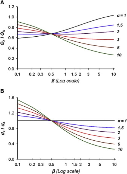
Genetic Diversity Ratio and Divergence Ratio as a Function of the Breeding Ratio at Different Values of α

Dependence of the X chromosome to the autosomes genetic diversity ratio Θ_X/Θ_A = 2(9β + 9)(2β + α)/(8β + 16)/(2β + 1)(α + 1) [A], and of the mutational divergence ratio $dX/dA=2\left(2\beta +\alpha \right)/\left(\alpha +1\right)\left(2\beta +1\right)$ [B] on the breeding ratio β for different α = μ_m/μ_f as indicated on the right of the graphs.

When α ≠ 1, the interspecies divergence ratios between the X chromosome and the autosomes, d_X/d_A (Figure 1), and between the sex chromosomes, d_X/d_Y (Equations A16 and A17 in Appendix A; Figure S8), are also dependent upon both α and β. When estimating α from the divergence ratios between the autosomes and the sex chromosomes it is important to correct for differences in the respective coalescence times of these chromosomes in the common ancestral population, proportionally extending their divergence time beyond the time of speciation.⁴⁴ The correction factor is ½Θ, which represents the average number of new sites that are expected to become fixed in one or the other of the species compared. If the present day values of Θ are used, we assume equal sizes of the present and ancestral populations. To estimate α, we considered a range of population sizes: 1 (an ancestral population size equal to the present one), 2, 3, and up to 4-fold greater.^6,8,45 Using human-chimpanzee d_X/d_A and human diversity data from genome-wide surveys,^43,46 we obtained estimates of α between 2.7 and 5.9, again assuming β between 1 and 1.4 and a range of ancestral population sizes (Table S3).

Discussion

Polygyny or Monogamy

Our estimates of the breeding ratio are close to but greater than 1, suggesting some polygyny in the history of human populations. Polygyny occurs when the reproductive variance of males is greater than that of females.³⁴ Greater variance implies that some males father more offspring than others. Excessive manifestations of polygyny are documented in the recent history of Asian populations,⁴⁷ but this may be the exception rather than the rule. Human beings are usually characterized as monogamous with polygamous tendencies.^1,11,35 Indeed, in approximately half of societies categorized as polygynous, only a small proportion of males (< 5%) take on more than one wife. Most populous contemporary societies are institutionally monogamous, leading to overall similar reproductive variance in men and women¹ However, more men than women do not marry and more men than women remarry after death or divorce, producing offspring in these later unions.¹¹ This so-called serial monogamy also applies to preagriculturalist societies¹⁰ and correlates with β greater than 1. Moreover, the generation time of men exceeds that of women by 13%–23%.⁴⁸ Integrated over a long evolutionary time, this effect could additionally inflate N_ef with respect to N_em and, by the same token, β, although this effect may be weakened as a result of a faster genetic drift of the X chromosomes transmitted by females.

Most nonhuman primates are polygynous, with males specializing in mating effort and females in parental effort. However, many higher primate males have a tendency to devote a greater proportion of their reproductive energy to offspring care, even if it occurs only at the group level. Maximizing parental care while minimizing number of offspring could have led to the increase in male parental investment favoring the development of a monogamous mating structure.¹² Mating structure is correlated with anatomical traits such as body-size dimorphism and the size of canines.^49,50 In higher primates, the degree of canine tooth dimorphisms is closely associated with the amount of direct competition among males for active access to females. Those species in which there is intense male-male competition, in comparison to female-female competition, are characterized by greater body-size dimorphism than those in which competition is lower in males or equal among the sexes. In humans, male-biased body-size dimorphism is only 1.15. This can be traced back to Australopithecus afarensis more than 3 million years ago and to Ardipithecus ramidus 4.4 million years ago, suggesting a shift toward monogamy already occurring in early hominids.^13,51 In summary, our finding of an overall breeding ratio close to but greater than 1 is consistent with conclusions from higher primate anatomical correlates of the mating structure^13,49,50 that suggest a shift toward monogamy while greater reproductive variance of males is maintained in the lineages leading to modern humans. Our results also concur with the analyses of evolutionary psychology and studies in anthropological demography describing humans as mildly polygynous or as monogamous with polygynous tendencies.^1,10,11,35

Interspecies Divergence Ratios and Genetic Diversities in the Context of α and β

Because population diversities and interspecies divergence ratios are essential for estimating α^7,8,41,42 and/or β,^3–5,52 and because α and β are interdependent, one has to consider β ≠ 1 when estimating α and α ≠ 1 when estimating β (Figure 2 and Figures S7 and S8). Graphs of Θ_X/Θ_A as a function of the breeding ratio β given different values of α are shown in Figure 2A. The effect of β on the ratio Θ_X/Θ_A is quite different depending on the value of α. Indeed, Θ_X/Θ_A increases with β when α < ∼1.5, it becomes almost independent of β at α ∼2, and it decreases with β at α > ∼2.5 (Figure 2). Thus, a reduction in Θ_X/Θ_A can reflect two situations: (1) a decrease in β when α is close to 1 (α < ∼ 1.5) or (2) an increase in β when α > ∼ 2.5. A similar phenomenon is observed for the evolutionary mutation rates, or interspecies divergence ratio of the X chromosome to the autosomes, d_X/d_A, which, when α ≠ 1, also becomes dependent upon β and always decreases with increasing β at α > 1 (Figure 2B).

In principle, this problem can be taken care of in the estimation of β by correcting the ratio of genetic diversities for differences in the mutation rates on the X chromosome and the autosomes by using an outgroup species. In practice, the correction differs depending on the choice of outgroup, such as chimpanzee, gorilla, orangutan, or macaque.^3,4,45,52 This is not surprising given that differences in α and β are probably present along different phylogenetic branches as a result of variations in generation length and/or differences in mating structure along lineages, such as those currently observed among living primates.^{12,40,41,49,50,53}

The only phylogenetic comparisons of the divergence rates that provide α estimates that do not depend on β, when β ≠ 1, are those between the autosomes and the Y chromosome (Equation A18). Unfortunately, the Y chromosome appears to evolve under effective purifying selection,⁹ such that the α estimates that rely on its evolutionary divergence may be strongly biased. Divergence between the X chromosome and the autosomes or between the X chromosome and the Y chromosome depend on both β and α (Figure 2A and Figure S8; Equations A18 and A17). Depending on the outgroup species, the connecting phylogenetic branches may be differently affected by variation in β, reflecting mating structures of the intermediate species, and by changes in α resulting from variation in generation length and other factors. Therefore, one has to be very cautious in using and interpreting such phylogenetic calibrations of chromosomal rate ratios because these may differ as a result of averaging over different levels of α and β along the lineages compared. The fact that many species are polygamous further emphasizes the need to consider the joint effect of β and α in evolutionary comparisons involving sex chromosomes.

Issues

Our values of $\widehat{\beta }$ range from 1.1 to 1.4 (Table 1), indicating a slight 10%–40% excess of breeding females per breeding male. They do not support the claim of a large excess of breeding females in the history of human populations.³ They seem to be more in line with the conclusions of those⁴ who suggest a population bottleneck and a decrease in the breeding ratio during out-of-Africa expansion. However, although we find ρ estimates substantially lower in non-Africans (Table 1), consistent with an important demographic bottleneck (Figure S5), our estimates of β are similar in Europeans and in Africans and lower only in Asians. The question is whether a reduced breeding ratio during a bottleneck, i.e., greater reduction in the number of breeding females than in the number of breeding males, could cause a sufficiently large decrease in N_eX/N_eA to account for the observations of Keinan et al.⁴ Using the inbreeding coefficients F estimated by these authors (Table S1 in ⁴), it is possible to express the relative strength of the autosomal and the X chromosome bottlenecks in terms of N_eX/N_eA. On the basis of these data, we calculate that N_eX/N_eA = 0.196 for North Europeans and that N_eX/N_eA = 0.259 for East Asians (Appendix B). Such values of N_eX/N_eA are well below the 9/16 limit of the ratio N_eX/N_eA when β tends toward 0 (Figure 1, Equation 6). However, assuming realistic β values, the shift in Θ_X/Θ_A observed by Keinan et al. could be explained provided that α > ∼2.5. On the other hand, mutations alone would not be sufficient to modify diversity patterns between the autosomes and the X chromosomes over a short period of evolutionary time. Therefore, selection or complex demography is a conceivable explanation, as suggested by the authors themselves.⁴ Complex demography is plausible, involving earlier population subdivisions within Africa itself^54–56 and/or subdivisions and founder effects during range expansion after the out-of-Africa bottleneck.⁵⁷

The divergence ratio d_X/d_A is independent of β at α = 1, whereas at α > 1, it always decreases when β increases (Figure 2B, Equation 16). The relatively low divergence ratio d_X/d_A between human and chimpanzee was interpreted in terms of “complex speciation of humans and chimpanzees.”⁵⁸ Instead, Wakeley⁵⁹ postulated greater α to explain this result. Indeed, increasing α lowers d_X/d_A, rendering the data more consistent with a simple speciation model. High α can itself account for a relatively low d_X/d_A, such that there would be no need to invoke postspeciation introgression of the X chromosome into lineage leading to humans,⁵⁸ as postulated by Hobolth et al.⁶⁰ Larger α along human and chimpanzee lineages than in other primates is plausible considering the relationship between generation time and α⁴¹ and the fact that human and chimpanzee generation times are the longest among primates, about 28 and 22 years, respectively^48,49,53 (e.g., more than two times longer than in Old World monkeys such as macaque). Using data sets from genome-wide sequencing or SNP surveys,⁴³ we estimated α between 2.7 and 5.9 (Tables S2 and S3), a plausible but relatively broad range of values that should be replicated with the use of different data sets.^8,41,61 Importantly for the discussion above, these estimates are greater than 2.5 (see Figure 2). In addition to α, our estimates of β will also benefit from the ongoing genome-wide genotyping and resequencing studies involving family trios and those using different methods of estimating ρ.³³

Estimation Protocol

We used a novel approach to assess the breeding ratio in humans that takes advantage of the fact that recombination on the X chromosome occurs only in females but occurs in both females and males on the autosomes. To evaluate β, we compared the autosomal population recombination rate to that of the X chromosome, estimated in three HapMap population samples^14,15 by the InfRec program.²¹ Importantly, our estimates of β do not require the knowledge of α and rely only on independently evaluated, average chromosomal recombination rates estimated from the pedigree studies.^18,19 Using both experimental and simulated data sets, we have previously shown that InfRec is a reliable tool for capturing fluctuations in recombination intensity due to recombination hotspots and is able to reveal overall differences in recombination rates and to faithfully capture quantitative differences between population samples.²¹ InfRec estimates rely on the RecMin's R_min values, which underestimate the number of historical recombinations. The extent to which InfRec underestimates the intrinsic population recombination rate can be tested through simulation experiments.²¹ These experiments demonstrate that about 40% of recombinations of the input ρ are being recovered in a simple population model and that the recovery rate changes with more complicated demography (Figures S3–S5). If the model is known, experimental estimates can subsequently be rescaled with the use of known recombination rates independently estimated from pedigree studies. This is not necessary when the ratios of the average ρ estimates between chromosomes or populations are sufficient, as in the case of the evaluation of the breeding ratio. Importantly, however, there is a very good correlation between chromosomal ρ_obs evaluated by InfRec in the three HapMap populations. This is also true between these ρ_obs and the chromosomal sex-average recombination rates estimated from pedigree studies (Figures S1 and S2). It shows that the population recombination rate inferred by InfRec reflects well the extent of recombinations in individual chromosomes observed at the pedigree level.

In simulation experiments, InfRec reliably recorded changes in the intensity of input ρ and these caused by demographic variations (Figures S3 and S6). A decrease in ρ was observed as a result of a demographic bottleneck as well as a result of population structure and inbreeding. This is consistent with earlier observation of an inflated linkage disequilibrium due to the same factors.³⁷ It was already shown that population bottleneck more profoundly affects the estimate of ρ than mutational diversity Θ.^21,62 In our simulations, in addition to ρ we also compared two estimates of Θ: the Watterson estimate Θ_S, based on the number of segregating sites,³⁰ and the Tajima estimate Θ_Π,³¹ summarizing sites' heterozygosity. The results show that because of the bottleneck, Θ_S suffers much more than Θ_Π. With an increasing number of generations after the bottleneck, estimates of ρ and Θ_S are asymptotically recovering to their prebottleneck values, contrasting Θ_Π that changes very slowly (Figure S5), and this process is accelerated by population growth. A faster recovery of Θ_S is comprehensible as each new mutation counts, irrespectively of the frequency of its new allele. The estimate of ρ relies on the same principle (Equation 11)¹⁷ as the Watterson estimate;³⁰ i.e., counting the number of events and dividing it by the length of the genealogical tree. This explains the similar behavior of these two parameters during and after the bottleneck.

Therefore, depending on the population demographic history, our estimates of ρ and subsequently β can be more or less affected by recent or ancient events. For example, we may expect that after an important population bottleneck, recent recombination history will weigh more than the ancient one, which would not be the case if the population evolved without drastic size changes. More data and analyses are needed to fully evaluate to what extent demographic history may bias our estimates of β. This would be especially important if there were substantial changes in reproductive behavior over evolutionary time, such as a shift from poly- to monogamy postulated from the analysis of the Y chromosome diversity.² In turn, the effect of migration, which depends on migration rate, differs for ρ and Θ. At high migration rate within a population composed of subpopulations, the estimates of ρ are similarly affected as the estimates of Θ, representing a sum of the subpopulation values, as if there were no population structure but only a single total population. When gene flow decreases, the coalescence of lineages that share their time among subpopulations becomes less probable. This extends the time to the most recent common ancestor and the length of the genealogy, leading thus to an increase in Θ estimates⁶³ (data not shown). The estimates of ρ by InfRec do not follow this trend and gradually decrease, consistent with an increase in linkage disequilibrium in a structured population.³⁷ This does not affect the ratio of ρ estimates and therefore the estimates of β unless the migration is sex biased. Over- or underestimated β values are observed when only females or only males are moving, respectively. This parallels the effect of sex-biased inbreeding and genetic differentiation, such as observed in patrilocal or matrilocal groups.^39,64 Although broad utility of our method to study sex-specific structure and social organization in human societies and other species still remains to be shown, the method certainly provides a complementary approach to studies comparing uniparentally transmitted markers and sequence diversities of the autosomes and X chromosome.^{3,4,38,39,64,65} As such, it may also provide new clues to the history of human populations, because it uses a type of information different than that based on mutational genetic record.

Appendix A. Population Diversity Ratios, Interspecies Divergence Ratios, and Interdependence of α and β

Genetic Diversity of the X Chromosome and the Autosomes

An autosomal sequence is derived from the mother and from the father with equal probability. Its rate of mutation is μ_A = (μ_f + μ_m)/2 per generation, in which subscripts f and m denote female and male germ line mutation rates, respectively, and their ratio is usually referred to as α = μ_m/μ_f.⁷

The population mutation rate is

$${\Theta }_A=4N_{eA}\frac{{\mu }_f+{\mu }_m}{2},$$ (Equation A1)

in which N_eA is the autosomal effective population size defined by Equation 2. At the breeding ratio β = N_f/N_m = 1, the X chromosome goes through the male meiosis one third of the time and through female meiosis two thirds of the time, such that the rate of mutation of an X-linked sequence in the population is μ_X = (2μ_f + μ_m)/3. For any β, μ_X = (2βμ_f + μ_m)/(2β + 1) and the population mutation rate for an X-linked sequence is

$${\Theta }_X=4N_{eX}\frac{2\beta {\mu }_f+{\mu }_m}{2\beta +1},$$ (Equation A2)

in which N_eX is the effective population size of X chromosomes defined by Equation 4 and δ = N_eX/N_eA by Equation 6. The ratio of genetic diversities between the X chromosome and the autosomes is thus

$$\frac{{\Theta }_X}{{\Theta }_A}=\frac{9\beta +9}{8\beta +16}·\frac{2\beta {\mu }_f+{\mu }_m}{2\beta +1}·\frac{2}{{\mu }_f+{\mu }_m},$$ (Equation A3)

or, defining α = μ_m/μ_f, we have

$$\frac{{\Theta }_X}{{\Theta }_A}=\frac{9\beta +9}{8\beta +16}·\frac{2\beta +\alpha }{2\beta +1}·\frac{2}{\alpha +1}\text{.}$$ (Equation A4)

Knowing Θ_X/Θ_A and β, we can calculate

$$\alpha =\frac{18\beta \left(\beta +1\right)-\frac{{\Theta }_X}{{\Theta }_A}\left(4\beta +8\right)\left(2\beta +1\right)}{\frac{{\Theta }_X}{{\Theta }_A}\left(4\beta +8\right)\left(2\beta +1\right)-9\left(\beta +1\right)},$$ (Equation A5)

and knowing α,

$$\beta =\frac{-20\frac{{\Theta }_X}{{\Theta }_A}\left(\alpha +1\right)+9\left(\alpha +2\right)\pm \sqrt{\Delta }}{16\frac{{\Theta }_X}{{\Theta }_A}\left(\alpha +1\right)-36},$$ (Equation A6)

in which $\Delta =144{\left({\Theta }_X/{\Theta }_A\right)}^2{\left(\alpha +1\right)}^2-72{\Theta }_X/{\Theta }_A\left(\alpha +1\right)\left(\alpha +2\right)+81{\left(\alpha +2\right)}^2-648\alpha$.

Genetic Diversity of the Y Chromosome Compared to the X Chromosome and the Autosomes

The genetic diversity of the Y chromosome, defined in terms of the population mutation rate, is

$${\Theta }_Y=2N_m{\mu }_m,$$ (Equation A7)

and thus the ratio of the Y chromosome to the X chromosome diversity is

$$\frac{{\Theta }_Y}{{\Theta }_X}=\frac{\beta +2}{9\beta }·\frac{\alpha \left(2\beta +1\right)}{2\beta +\alpha },$$ (Equation A8)

from which

$$\alpha =\frac{18{\beta }^2\frac{{\Theta }_Y}{{\Theta }_X}}{\left(\beta +2\right)\left(2\beta +1\right)-9\beta \frac{{\Theta }_Y}{{\Theta }_X}}\text{.}$$ (Equation A9)

The Y chromosome-to-autosomes genetic diversity ratio is

$$\frac{{\Theta }_Y}{{\Theta }_A}=\frac{\beta +1}{8\beta }·\frac{2\alpha }{\alpha +1},$$ (Equation A10)

and thus, assuming neutrality, one can again calculate

$$\alpha =\frac{8\beta \frac{{\Theta }_Y}{{\Theta }_A}}{2\left(\beta +1\right)-8\beta \frac{{\Theta }_Y}{{\Theta }_A}}\text{.}$$ (Equation A11)

Interspecies Divergence Data

We can also derive expressions to estimate α from interspecies divergence data. Taking μ_A = (μ_f + μ_m)/2, μ_X = (2βμ_f + μ_m)/(2β + 1), and μ_Y + μ_m, we obtain

$${\mu }_m={\mu }_A\frac{2\alpha }{\alpha +1}$$ (Equation A12)

and

$${\mu }_f={\mu }_A\frac{2}{\alpha +1},$$ (Equation A13)

and thus

$${\mu }_X=2{\mu }_A\frac{2\beta +\alpha }{\left(\alpha +1\right)\left(2\beta +1\right)}$$ (Equation A14)

and

$${\mu }_Y={\mu }_A\frac{2\alpha }{\alpha +1},$$ (Equation A15)

from which, assuming neutrality, interspecies divergence ratios between the sex chromosomes and the autosomes are as follows

$$\frac{d_X}{d_A}=\frac{2\left(2\beta +\alpha \right)}{\left(\alpha +1\right)\left(2\beta +1\right)},$$ (Equation A16)

$$\frac{d_X}{d_Y}=\frac{2\beta +\alpha }{\alpha \left(2\beta +1\right)},$$ (Equation A17)

and

$$\frac{d_A}{d_Y}=\frac{1+\alpha }{2\alpha },$$ (Equation A18)

and the corresponding formulas for estimating α are

$$\alpha =\frac{1}{2\left(d_A/d_Y\right)-1},$$ (Equation A19)

$$\alpha =\frac{\left(d_X/d_A\right)\left(2\beta +1\right)-4\beta }{2-\left(d_X/d_A\right)\left(2\beta +1\right)},$$ (Equation A20)

and

$$\alpha =\frac{2\beta }{\left(d_X/d_Y\right)\left(2\beta +1\right)-1}\text{.}$$ (Equation A21)

Thus, importantly, we always have to consider β in the evaluation of α when using genetic diversity data, and the same applies to interspecies comparisons, except when comparing divergence of the autosomes with that of the Y chromosome.

Appendix B. Lower Limit of N_eX/N_eA

The inbreeding coefficient F is used to measure the intensity of a population bottleneck: F = 1 −(1 − 1/2N_eb)^g, in which 2N_eb represents the number of chromosomes during a bottleneck that lasts g generations. With estimates of F for the autosomes, F_A (when 2N_eb = N_eA), and the X chromosome, F_X (when 2N_eb = N_eX), we can calculate the ratio as N_eX/N_eA = ln(1 − F_A)/ln(1 − F_X).

Using the inbreeding coefficient estimates of Keinan et al. (2009)⁴ (see their Table S1) and assuming the same bottleneck duration for the X chromosome and the autosomes, we obtain N_eX/N_eA = 0.196 for North Europeans and N_eX/N_eA = 0.259 for East Asians. Assuming neutrality, such a reduction of N_eX/N_eA is beyond its lowest limit of 9/16, with β tending toward 0 (N_eX/N_eA = (9β + 9)/(8β + 16)).

Web Resources

The URLs for the data presented herein are as follows:

• International HapMap Project, http://www.hapmap.org/

• ms Simulation Program, http://home.uchicago.edu/∼rhudson1/source/mksamples.html

References

- 1.Brown G.R., Laland K.N., Mulder M.B. Bateman's principles and human sex roles. Trends Ecol. Evol. 2009;24:297–304. doi: 10.1016/j.tree.2009.02.005. [DOI] [PMC free article] [PubMed] [Google Scholar]
- 2.Dupanloup I., Pereira L., Bertorelle G., Calafell F., Prata M.J., Amorim A., Barbujani G. A recent shift from polygyny to monogamy in humans is suggested by the analysis of worldwide Y-chromosome diversity. J. Mol. Evol. 2003;57:85–97. doi: 10.1007/s00239-003-2458-x. [DOI] [PubMed] [Google Scholar]
- 3.Hammer M.F., Mendez F.L., Cox M.P., Woerner A.E., Wall J.D. Sex-biased evolutionary forces shape genomic patterns of human diversity. PLoS Genet. 2008;4:e1000202. doi: 10.1371/journal.pgen.1000202. [DOI] [PMC free article] [PubMed] [Google Scholar]
- 4.Keinan A., Mullikin J.C., Patterson N., Reich D. Accelerated genetic drift on chromosome X during the human dispersal out of Africa. Nat. Genet. 2009;41:66–70. doi: 10.1038/ng.303. [DOI] [PMC free article] [PubMed] [Google Scholar]
- 5.Bustamante C.D., Ramachandran S. Evaluating signatures of sex-specific processes in the human genome. Nat. Genet. 2009;41:8–10. doi: 10.1038/ng0109-8. [DOI] [PMC free article] [PubMed] [Google Scholar]
- 6.Makova K.D., Li W.H. Strong male-driven evolution of DNA sequences in humans and apes. Nature. 2002;416:624–626. doi: 10.1038/416624a. [DOI] [PubMed] [Google Scholar]
- 7.Miyata T., Hayashida H., Kuma K., Mitsuyasu K., Yasunaga T. Male-driven molecular evolution: a model and nucleotide sequence analysis. Cold Spring Harb. Symp. Quant. Biol. 1987;52:863–867. doi: 10.1101/sqb.1987.052.01.094. [DOI] [PubMed] [Google Scholar]
- 8.Taylor J., Tyekucheva S., Zody M., Chiaromonte F., Makova K.D. Strong and weak male mutation bias at different sites in the primate genomes: insights from the human-chimpanzee comparison. Mol. Biol. Evol. 2006;23:565–573. doi: 10.1093/molbev/msj060. [DOI] [PubMed] [Google Scholar]
- 9.Rozen S., Marszalek J.D., Alagappan R.K., Skaletsky H., Page D.C. Remarkably little variation in proteins encoded by the Y chromosome's single-copy genes, implying effective purifying selection. Am. J. Hum. Genet. 2009;85:923–928. doi: 10.1016/j.ajhg.2009.11.011. [DOI] [PMC free article] [PubMed] [Google Scholar]
- 10.Frost P. Sexual selection and human geaographic variation. Journal of Social. Evolutionary and Cultural Psychology. 2008;2:169–191. [Google Scholar]
- 11.Low B.S. A Darwinian Look at Human Behavior. Princeton University Press; Princeton, Oxford: 2000. Why Sex Matters. [Google Scholar]
- 12.Lovejoy C.O. The Origin of Man. Science. 1981;211:341–350. doi: 10.1126/science.211.4480.341. [DOI] [PubMed] [Google Scholar]
- 13.Reno P.L., Meindl R.S., McCollum M.A., Lovejoy C.O. Sexual dimorphism in Australopithecus afarensis was similar to that of modern humans. Proc. Natl. Acad. Sci. USA. 2003;100:9404–9409. doi: 10.1073/pnas.1133180100. [DOI] [PMC free article] [PubMed] [Google Scholar]
- 14.International HapMap Consortium The International HapMap Project. Nature. 2003;426:789–796. doi: 10.1038/nature02168. [DOI] [PubMed] [Google Scholar]
- 15.Consortium T.I.H., International HapMap Consortium A haplotype map of the human genome. Nature. 2005;437:1299–1320. doi: 10.1038/nature04226. [DOI] [PMC free article] [PubMed] [Google Scholar]
- 16.Frazer K.A., Ballinger D.G., Cox D.R., Hinds D.A., Stuve L.L., Gibbs R.A., Belmont J.W., Boudreau A., Hardenbol P., Leal S.M., International HapMap Consortium A second generation human haplotype map of over 3.1 million SNPs. Nature. 2007;449:851–861. doi: 10.1038/nature06258. [DOI] [PMC free article] [PubMed] [Google Scholar]
- 17.Hein J., Schierup M., Wiuf C. A Primer in Coalescent Theory. Oxford University Press; Oxford: 2005. Gene Genealogies, Variation and Evolution. [Google Scholar]
- 18.Kong A., Gudbjartsson D.F., Sainz J., Jonsdottir G.M., Gudjonsson S.A., Richardsson B., Sigurdardottir S., Barnard J., Hallbeck B., Masson G. A high-resolution recombination map of the human genome. Nat. Genet. 2002;31:241–247. doi: 10.1038/ng917. [DOI] [PubMed] [Google Scholar]
- 19.Kong X., Murphy K., Raj T., He C., White P.S., Matise T.C. A combined linkage-physical map of the human genome. Am. J. Hum. Genet. 2004;75:1143–1148. doi: 10.1086/426405. [DOI] [PMC free article] [PubMed] [Google Scholar]
- 20.Caballero A. Developments in the prediction of effective population size. Heredity. 1994;73:657–679. doi: 10.1038/hdy.1994.174. [DOI] [PubMed] [Google Scholar]
- 21.Lefebvre J.F., Labuda D. Fraction of informative recombinations: a heuristic approach to analyze recombination rates. Genetics. 2008;178:2069–2079. doi: 10.1534/genetics.107.082255. [DOI] [PMC free article] [PubMed] [Google Scholar]
- 22.Stephens M., Smith N.J., Donnelly P. A new statistical method for haplotype reconstruction from population data. Am. J. Hum. Genet. 2001;68:978–989. doi: 10.1086/319501. [DOI] [PMC free article] [PubMed] [Google Scholar]
- 23.Myers S.R., Griffiths R.C. Bounds on the minimum number of recombination events in a sample history. Genetics. 2003;163:375–394. doi: 10.1093/genetics/163.1.375. [DOI] [PMC free article] [PubMed] [Google Scholar]
- 24.Zietkiewicz E., Yotova V., Gehl D., Wambach T., Arrieta I., Batzer M., Cole D.E.C., Hechtman P., Kaplan F., Modiano D. Haplotypes in the dystrophin DNA segment point to a mosaic origin of modern human diversity. Am. J. Hum. Genet. 2003;73:994–1015. doi: 10.1086/378777. [DOI] [PMC free article] [PubMed] [Google Scholar]
- 25.Hudson R.R., Kaplan N.L. Statistical properties of the number of recombination events in the history of a sample of DNA sequences. Genetics. 1985;111:147–164. doi: 10.1093/genetics/111.1.147. [DOI] [PMC free article] [PubMed] [Google Scholar]
- 26.Efron B., Tibshirani R.J. Chapman & Hall; New York: 1993. An introduction to the bootstrap. [Google Scholar]
- 27.Hellenthal G., Stephens M. msHOT: modifying Hudson's ms simulator to incorporate crossover and gene conversion hotspots. Bioinformatics. 2007;23:520–521. doi: 10.1093/bioinformatics/btl622. [DOI] [PubMed] [Google Scholar]
- 28.Hudson R.R. Gene Genealogies and the Coalescent Process. Oxford Surveys in Evolutionary Biology. 1990;7:1–44. [Google Scholar]
- 29.Li J., Zhang M.Q., Zhang X. A new method for detecting human recombination hotspots and its applications to the HapMap ENCODE data. Am. J. Hum. Genet. 2006;79:628–639. doi: 10.1086/508066. [DOI] [PMC free article] [PubMed] [Google Scholar]
- 30.Watterson G.A. On the number of segregating sites in genetical models without recombination. Theor. Popul. Biol. 1975;7:256–276. doi: 10.1016/0040-5809(75)90020-9. [DOI] [PubMed] [Google Scholar]
- 31.Tajima F. Statistical method for testing the neutral mutation hypothesis by DNA polymorphism. Genetics. 1989;123:585–595. doi: 10.1093/genetics/123.3.585. [DOI] [PMC free article] [PubMed] [Google Scholar]
- 32.Hudson R.R. Generating samples under a Wright-Fisher neutral model of genetic variation. Bioinformatics. 2002;18:337–338. doi: 10.1093/bioinformatics/18.2.337. [DOI] [PubMed] [Google Scholar]
- 33.Stumpf M.P., McVean G.A. Estimating recombination rates from population-genetic data. Nat. Rev. Genet. 2003;4:959–968. doi: 10.1038/nrg1227. [DOI] [PubMed] [Google Scholar]
- 34.Bateman A.J. Intra-sexual selection in Drosophila. Heredity. 1948;2:349–368. doi: 10.1038/hdy.1948.21. [DOI] [PubMed] [Google Scholar]
- 35.Scheidel, W. (2009). Monogamy and Polygyny. Princeton/Stanford Working Papers in Classics Version 1, 1–14.
- 36.Pool J.E., Nielsen R. Population size changes reshape genomic patterns of diversity. Evolution. 2007;61:3001–3006. doi: 10.1111/j.1558-5646.2007.00238.x. [DOI] [PMC free article] [PubMed] [Google Scholar]
- 37.Pritchard J.K., Przeworski M. Linkage disequilibrium in humans: models and data. Am. J. Hum. Genet. 2001;69:1–14. doi: 10.1086/321275. [DOI] [PMC free article] [PubMed] [Google Scholar]
- 38.Seielstad M.T., Minch E., Cavalli-Sforza L.L. Genetic evidence for a higher female migration rate in humans. Nat. Genet. 1998;20:278–280. doi: 10.1038/3088. [DOI] [PubMed] [Google Scholar]
- 39.Ségurel L., Martínez-Cruz B., Quintana-Murci L., Balaresque P., Georges M., Hegay T., Aldashev A., Nasyrova F., Jobling M.A., Heyer E., Vitalis R. Sex-specific genetic structure and social organization in Central Asia: insights from a multi-locus study. PLoS Genet. 2008;4:e1000200. doi: 10.1371/journal.pgen.1000200. [DOI] [PMC free article] [PubMed] [Google Scholar]
- 40.Goetting-Minesky M.P., Makova K.D. Mammalian male mutation bias: impacts of generation time and regional variation in substitution rates. J. Mol. Evol. 2006;63:537–544. doi: 10.1007/s00239-005-0308-8. [DOI] [PubMed] [Google Scholar]
- 41.Hedrick P.W. Sex: differences in mutation, recombination, selection, gene flow, and genetic drift. Evolution. 2007;61:2750–2771. doi: 10.1111/j.1558-5646.2007.00250.x. [DOI] [PubMed] [Google Scholar]
- 42.Ellegren H. The different levels of genetic diversity in sex chromosomes and autosomes. Trends Genet. 2009;25:278–284. doi: 10.1016/j.tig.2009.04.005. [DOI] [PubMed] [Google Scholar]
- 43.Sachidanandam R., Weissman D., Schmidt S.C., Kakol J.M., Stein L.D., Marth G., Sherry S., Mullikin J.C., Mortimore B.J., Willey D.L., International SNP Map Working Group A map of human genome sequence variation containing 1.42 million single nucleotide polymorphisms. Nature. 2001;409:928–933. doi: 10.1038/35057149. [DOI] [PubMed] [Google Scholar]
- 44.Ebersberger I., Metzler D., Schwarz C., Pääbo S. Genomewide comparison of DNA sequences between humans and chimpanzees. Am. J. Hum. Genet. 2002;70:1490–1497. doi: 10.1086/340787. [DOI] [PMC free article] [PubMed] [Google Scholar]
- 45.Burgess R., Yang Z. Estimation of hominoid ancestral population sizes under bayesian coalescent models incorporating mutation rate variation and sequencing errors. Mol. Biol. Evol. 2008;25:1979–1994. doi: 10.1093/molbev/msn148. [DOI] [PubMed] [Google Scholar]
- 46.Chimpanzee Sequencing and Analysis Consortium Initial sequence of the chimpanzee genome and comparison with the human genome. Nature. 2005;437:69–87. doi: 10.1038/nature04072. [DOI] [PubMed] [Google Scholar]
- 47.Zerjal T., Xue Y., Bertorelle G., Wells R.S., Bao W., Zhu S., Qamar R., Ayub Q., Mohyuddin A., Fu S. The genetic legacy of the Mongols. Am. J. Hum. Genet. 2003;72:717–721. doi: 10.1086/367774. [DOI] [PMC free article] [PubMed] [Google Scholar]
- 48.Fenner J.N. Cross-cultural estimation of the human generation interval for use in genetics-based population divergence studies. Am. J. Phys. Anthropol. 2005;128:415–423. doi: 10.1002/ajpa.20188. [DOI] [PubMed] [Google Scholar]
- 49.Fleagle J.G. Academic Press, Inc.; San Diego: 1988. Primate Adaptation & Evolution. [Google Scholar]
- 50.Jones S., Martin R., Pilbeam D. The Cambridge Encyclopedia of Human Evolution. In: Bunney S., editor. Cambridge. Cambridge University Press; Cambridge, UK: 1992. [Google Scholar]
- 51.Lovejoy C.O. Reexamining human origins in light of Ardipithecus ramidus. Science. 2009;326:71–78. [PubMed] [Google Scholar]
- 52.Innan H., Watanabe H. The effect of gene flow on the coalescent time in the human-chimpanzee ancestral population. Mol. Biol. Evol. 2006;23:1040–1047. doi: 10.1093/molbev/msj109. [DOI] [PubMed] [Google Scholar]
- 53.Gage T.B. The comparative demography of primates: with some comments on the evolution of life histories. Annu. Rev. Anthropol. 1998;27:197–221. doi: 10.1146/annurev.anthro.27.1.197. [DOI] [PubMed] [Google Scholar]
- 54.Labuda D., Zietkiewicz E., Yotova V. Archaic lineages in the history of modern humans. Genetics. 2000;156:799–808. doi: 10.1093/genetics/156.2.799. [DOI] [PMC free article] [PubMed] [Google Scholar]
- 55.Yotova V., Lefebvre J.F., Kohany O., Jurka J., Michalski R., Modiano D., Utermann G., Williams S.M., Labuda D. Tracing genetic history of modern humans using X-chromosome lineages. Hum. Genet. 2007;122:431–443. doi: 10.1007/s00439-007-0413-4. [DOI] [PubMed] [Google Scholar]
- 56.Harding R.M., McVean G. A structured ancestral population for the evolution of modern humans. Curr. Opin. Genet. Dev. 2004;14:667–674. doi: 10.1016/j.gde.2004.08.010. [DOI] [PubMed] [Google Scholar]
- 57.Pool J.E., Nielsen R. The impact of founder events on chromosomal variability in multiply mating species. Mol. Biol. Evol. 2008;25:1728–1736. doi: 10.1093/molbev/msn124. [DOI] [PMC free article] [PubMed] [Google Scholar]
- 58.Patterson N., Richter D.J., Gnerre S., Lander E.S., Reich D. Genetic evidence for complex speciation of humans and chimpanzees. Nature. 2006;441:1103–1108. doi: 10.1038/nature04789. [DOI] [PubMed] [Google Scholar]
- 59.Wakeley J. Complex speciation of humans and chimpanzees. Nature. 2008;452:E3–E4. doi: 10.1038/nature06805. [DOI] [PubMed] [Google Scholar]
- 60.Hobolth A., Christensen O.F., Mailund T., Schierup M.H. Genomic relationships and speciation times of human, chimpanzee, and gorilla inferred from a coalescent hidden Markov model. PLoS Genet. 2007;3:e7. doi: 10.1371/journal.pgen.0030007. [DOI] [PMC free article] [PubMed] [Google Scholar]
- 61.Ellegren H. Characteristics, causes and evolutionary consequences of male-biased mutation. Proc Biol Sci. 2007;274:1–10. doi: 10.1098/rspb.2006.3720. [DOI] [PMC free article] [PubMed] [Google Scholar]
- 62.Thornton K., Andolfatto P. Approximate Bayesian inference reveals evidence for a recent, severe bottleneck in a Netherlands population of Drosophila melanogaster. Genetics. 2006;172:1607–1619. doi: 10.1534/genetics.105.048223. [DOI] [PMC free article] [PubMed] [Google Scholar]
- 63.Wakeley J. Roberts & Company Publishers; Greenwood Village, Colorado: 2009. Coalescent Theory: An Introduction. [Google Scholar]
- 64.Wilkins J.F., Marlowe F.W. Sex-biased migration in humans: what should we expect from genetic data? Bioessays. 2006;28:290–300. doi: 10.1002/bies.20378. [DOI] [PubMed] [Google Scholar]
- 65.Wilder J.A., Kingan S.B., Mobasher Z., Pilkington M.M., Hammer M.F. Global patterns of human mitochondrial DNA and Y-chromosome structure are not influenced by higher migration rates of females versus males. Nat. Genet. 2004;36:1122–1125. doi: 10.1038/ng1428. [DOI] [PubMed] [Google Scholar]
Associated Data
This section collects any data citations, data availability statements, or supplementary materials included in this article.