Struct-NB: Predicting Protein-RNA Binding Sites Using Structural Features

Abstract

We explore whether protein-RNA interfaces differ from non-interfaces in terms of their structural features and whether structural features vary according to the type of the bound RNA (e.g., mRNA, siRNA, etc.), using a non-redundant dataset of 147 protein chains extracted from protein-RNA complexes in the Protein Data Bank. Furthermore, we use machine learning algorithms for training classifiers to predict protein-RNA interfaces using information derived from the sequence and structural features. We develop the Struct-NB classifier that takes into account structural information. We compare the performance of Naïve Bayes and Gaussian Naïve Bayes with that of Struct-NB classifiers on the 147 protein-RNA dataset using sequence and structural features respectively as input to the classifiers. The results of our experiments show that Struct-NB outperforms Naïve Bayes and Gaussian Naïve Bayes on the problem of predicting the protein-RNA binding interfaces in a protein sequence in terms of a range of standard measures for comparing the performance of classifiers.

1 Introduction

Protein-RNA interactions play a vital role in RNA splicing, translation, replication of many viruses as well as many other processes in the cell. The prediction of protein-RNA interfaces can aid in the design of drug-inhibitors for viruses, down-regulation of unwanted genes as well as contributing to our basic understanding of the mechanisms involved in protein-RNA recognition [Moore, 2005, Noller, 2005, Jurica and Moore, 2003, Freed and Mouland, 2006]. At least nine families of RNA-binding proteins have been identified using sequence-based analyses of the major groups of RNA-binding proteins, together with functional characterization of mutations that affect the specificity or affinity of RNA binding (for review, see [Chen and Varani, 2005]). In contrast, the number of experimentally determined structures for protein-RNA complexes is still relatively small and heavily biased (ribosomal proteins represent 50% of all RNA binding proteins in the Protein Data Bank [PDB] [Berman et al., 2000]).

Because of the importance of protein-RNA interactions in biological regulation and the considerable effort required to identify RNA binding residues through biophysical analyses of protein-RNA complexes or in vitro binding studies, there is an urgent need for computational methods to identify RNA binding sites given a protein’s primary amino acid sequence, and when available, its 3-dimensional structure. Several recent studies have focused on the development of machine learning approaches to amino acid sequence-based prediction of RNA-binding residues in proteins [Terribilini et al., 2007, Terribilini et al., 2006b, Jeong et al., 2004, Jeong and Miyano, 2006]. The predictions obtained using such methods have already contributed to the design of wet-lab experiments to decipher mechanisms of protein-RNA recognition [Terribilini et al., 2006a, Bechara et al., 2007]. However, the machine learning approaches to prediction of RNA-binding residues of proteins have focused largely on the analysis of amino acid sequence as opposed to the structural features of the protein chain. Other analyses of protein-RNA interfaces [Jones et al., 2001, M and E, 2001, Lejeune et al., 2005] have focused on the analysis of hydrogen bonds or van der Waals contacts in between the protein and the RNA. There has been relatively little attention paid to structural features of the interface (e.g protrusion or roughness) rather than the atomic forces.

Against this background, it is natural to ask: Do protein-RNA interfaces differ from non-interfaces in terms of their structural features? Do the structural features vary according to the type of the bound RNA (e.g., mRNA, siRNA etc.)? Can structural features be utilized to improve classification performance of protein-RNA interfaces relative to sequence-based classifiers? If we find that the protein-RNA interfaces differ from noninterfaces in terms of their structural features, then the structural features can be exploited by machine learning approaches to predict protein-RNA interface residues when the structure of the protein is available but the structures of the complexes formed by the protein with RNA are not. If the different classes of protein-RNA interfaces significantly differ from each other with respect to their structural features, it might be possible to improve the specificity and sensitivity of protein-RNA interface residue prediction by training separate classifiers for each type of bound RNA.

We describe an analysis of the structural features of protein chains from RNA-binding proteins that explores this question using a non-redundant dataset of 147 protein chains from the RB147 dataset [Terribilini et al., 2007]. We focus on two of the six structural properties of amino acid residues used in a recent analysis of protein-protein interfaces by Wu et al. [Wu et al., 2007], namely, surface roughness [Lewis and Rees, 1985] and CX value [Pintar et al., 2002]. Solid Angle [Connolly, 1986] was also used early in this study (see [Towfic et al., 2007]). However, it was deemed unnecessary to include in this study since the results from Solid Angle overlap with those of Roughness [Lewis and Rees, 1985] with a correlation of 0.88 (roughness and CX overlap with a correlation of −0.56).

The results of our analysis show that protein-RNA interface residues tend to be protruding compared to non-interface residues. Furthermore, interface residues tend to have rough surfaces. Our analysis also shows that the protein chains in protein-RNA interfaces containing Viral-RNA and rRNA significantly differ from those that contain dsRNA, mRNA, siRNA, snRNA, SRP RNA and tRNA with respect to their CX values. We developed Struct-NB classifiers to demostrate the utilization of the structural features in predicting protein-RNA interface residues in a protein sequence.

The rest of the paper is organized as follows: Section 2 describes the RB147 dataset and each of 2 properties of amino acid residues examined in this study as well as the methods used in the construction and evaluation of the Struct-NB classifier. Section 3 presents the results of our analysis, comparing interface and noninterface residues based on these two properties and comparing the various Naïve Bayes and Struct-NB classifiers constructed using sequence and structural features. Section 4 concludes with a summary and an outline of some directions for further research.

2 Materials and Methods

2.1 Dataset

The RB147 dataset [Terribilini et al., 2007] used in this study contains protein chains extracted from structures of protein-RNA complexes in the PDB solved by X-ray crystallography, after eliminating protein chains from structures with resolution worse than 3.5Å and protein chains sharing a sequence identity greater than 30% with one or more other protein chains. The RB147 dataset contains 147 non-redundant protein chains and a total of 32,324 amino acids. The RNA-binding residues are defined as follows: an RNA-binding residue is an amino acid containing at least one atom within 5Å of any atom in the bound RNA. According to this definition, RB147 contains a total of 6,157 RNA-binding residues and 26,167 non-binding residues.

2.2 Classification of the Protein Chains Based on the Type of the Bound RNA

The protein chains in the RB147 dataset were classified into 9 classes according to the type(s) of RNA that was found in the corresponding protein-RNA complex based on a taxonomy of RNA types used previously by Ellis et al. [Ellis et al., 2007]: dsRNA, mRNA, rRNA, siRNA, snRNA, SRP RNA, tRNA, Viral RNA or “other” (which denoted synthetic RNAs or pre-mRNAs or a class of RNAs not included in any of the other categories). The classification for each PDB id and chain in the dataset is shown in table 1. Over half of the protein chains belong to complexes with rRNA, with tRNA, mRNA and viral RNA being the other dominant groups (in that order).

Table 1.

Classification for each of the 147 protein chains in the dataset. The four letter PDB ids are subscripted by the chain. As can be seen from the table, over half (55.7%) of the RNAs are rRNAs.

RNA Type	PDBIDs
dsRNA	1DI2A; 1UV JA; 1Y Z9A
mRNA	1AV 6A; 1G2EA; 1GTFQ; 1KNZA 1KQ2A; 1M 8XA; 1WPUA; 1WSUA 2A1RA; 2ASBA
rRNA	1APGA; 1DFUP ; 1FEUA; 1FJGB 1FJGC; 1FJGD; 1FJGE; 1FJGG 1FJGI; 1FJGJ; 1FJGK; 1FJGL 1FJGM ; 1FJGN ; 1FJGP ; 1FJGQ 1FJGS; 1FJGT ; 1FJGV ; 1G1XA 1HROW ; 1I6UA; 1JBRA; 1MZPA 1SDSA; 1T 0KB; 1UN 6B; 1V QO1 1V QO2; 1V QO3; 1V QOA; 1V QOB 1V QOC; 1V QOD; 1V QOE; 1V QOG 1V QOH; 1V QOI; 1V QOJ; 1V QOK 1V QOL; 1V QOM ; 1V QON ; 1V QOP 1V QOQ; 1V QOR; 1V QOS; 1V QOT 1V QOU ; 1V QOV ; 1V QOW ; 1V QOX 1V QOY ; 1V QOZ; 1W 2B5; 1Y 698 1Y 69K; 1Y 69U ; 2AV YF ; 2AV YU 2AW40; 2AW 41; 2AW 42; 2AW 43 2AW4D; 2AW 4E; 2AW 4G; 2AW 4H 2AW4J; 2AW 4L; 2AW 4N ; 2AW 4P 2AW4Q; 2AW 4R; 2AW 4S; 2AW 4Y 2AW4Z; 2BH2A; 2D3O1; 2D3OS 1G1XB; 1G1XC
siRNA	1RPUA; 1SI3A; 2BGGA
snRNA	1A9NA; 1EC6A; 1LNGA; 1M 8VA 1OOAA
SRP RNA	1E8OA; 1HQ1A
tRNA	1ASYA; 1B23P ; 1C0AA; 1EIYB 1F7UA; 1FFYA; 1H3EA; 1H4SA 1J1UA; 1J2BA; 1K8WA; 1N 78A 1Q2SA; 1QF 6A; 1QTQA; 1R3EA 1SERA; 1TFWA; 1U 0BB; 1V FGA 1WZ2A; 2BTEA; 2CT 8A; 2FMTA
Viral RNA	1A34A; 1DDLA; 1H2CA; 1LAJA 1N35A; 1NB7A; 1PGL2; 1RMVA 1WNEA;2AZ0A; 2BU 1A
Other	1B2MA; 1JIDA; 1M 5OC; 1Y V PA 1ZH5A; 2A8VA; 2BX2L

2.3 Analysis of Structural Properties

Each chain in the dataset was analyzed in terms of its surface roughness [Lewis and Rees, 1985]and CX value [Pintar et al., 2002]. The analysis was repeated on subsets of the dataset corresponding to the classification based on the type of the RNA found in the interface (see table 1). We implemented a program in Java, Structure-Analyzer 1.0 (available at http://www.public.iastate.edu/~ftowfic) for this analysis. The Java package has an easy-to-use API to allow its use in other applications. The program generates a standard tab-delimited output file with the PDBID, chain name, residue name (three letter abbreviation), residue number, a + or − indicating whether or not the residue is part of the interface, a score derived from the structural property being examined (roughness and cx) and a + or − denoting whether or not the residue is part of the surface of the protein (the definition of a surface residue can be varied within the class as desired). In our analysis, surface residues are defined as residues that have a solvent accessible surface area that is at least 5% of their total surface area [Wu et al., 2007, Connolly, 1993].

2.4 Roughness Calculation

The roughness value for a residue denotes the degree of irregularity of that point at the surface as outlined by Lewis et al. and Lee et al. [Lewis and Rees, 1985, Lee and Richards, 1971]. The surface roughness value (D) is given by:

$$D=2-\frac{\partial log{A}_s}{\partial logR}$$

The roughness calculation requires a molecule surface area (A_s), which is obtained by rolling a sphere with radius R against the protein and calculating the area of the resulting surface as implemented in the MSP software package [Connolly, 1993]. The radius R of the sphere is varied from 0.2 to 4.0Å in 0.1 increments. Thus, we get the surface area for each choice of the radius which in turn can be used to calculate the partial derivative $\frac{\partial log{A}_s}{\partial logR}$ for each residue. Thus, a final roughness value (D) is associated with each residue on the surface of the protein. For a perfectly smooth surface D = 2 whereas for a rough surface, D > 2.

2.5 CX Value Calculation

The CX value measures the ratio of the volume of atoms that occupy a 6Å sphere compared to the empty volume within the sphere [Pintar et al., 2002]. The CX score is calculated by centering a 6Å sphere around an atom and calculating the CX value based on the volume of neighboring atoms according to the formula:

$$CX=\frac{\mathit{Unoccupied}\mathit{volume}of\mathit{the}6\mathring{A}\mathit{sphere}}{\mathit{Total}\mathit{volume}of\mathit{atoms}\mathit{that}\mathit{occupy}\mathit{the}6\mathring{A}\mathit{sphere}}$$

The CX value is calculated for each atom in the surface residues. The CX score for a residue can be calculated using three different methods: First, the CX score can be extracted from the alpha-carbon atom and that score is used for the whole residue (alphacarbon method). A second method is to simply average the CX score across all atoms for the residue and use the average score as the CX score for the residue (averagecx method). Finally, the CX scores for the atoms in the R-group of the residue can be averaged and that average can be used as the CX score for the residue (rgroup method). The CX score ranges from 0 (for residues that are non-protruding) to 15 (for residues that are highly protruding from the protein surface).

2.6 Interface Propensity Calculations

Consider a residue-based property (such as residue roughness) with k discrete values: (v₁, v₂,..., v_k). Each surface residue is assigned to one of k disjoint subsets S₁, S₂,..., S_k based on the value of the residue property. Let I_i and N_i respectively be the fractions of interface residues and non-interface residues in the set S_i. Let I and N respectively denote the fractions of interface and non-interface residues in the entire dataset (over all of the score ranges). The log-propensity for the interface can then be expressed by:

$$I{P}_i={log}_2({\mathit{Propensity}}_i)=lo{g}_2(\frac{\frac{I_i}{I}}{\frac{I_i+N_i}{I+N}})$$

The interface propensity IP_i of the property at value v_i is a measure of the preference for the value (or a range of values) v_i among the interface residues (relative to the entire set of surface residues). IP_i > 0 denotes that the specified property value (or a range of values) v_i tends to be more preferred among the interface residues relative to the surface residues. Similarly, IP_i < 0 denotes that the specified property value v_i tends to be less preferred among the interface residues relative to the entire set of surface residues.

2.7 Predicting Protein-RNA Interfaces Using Machine Learning Approaches

The problem of identifying protein-RNA interface residues in a protein sequence can be formulated as a binary classification problem: Given a sequence S of length N, S = s₁s₂ · · ·s_N over the alphabet Σ of amino acids, s_i ∈ Σ,i = 1, · · ·, N and S ∈ Σ*, the task is to predict whether or not a residue in the sequence is protein-RNA interface residue.

One particular challenge in training classifiers using standard machine learning algorithms is to capture predictive “features” that result in accurate classification of new examples. Hence, in this study, we explored sequence and structural features as input to the classifiers trained to label each residue in a protein-RNA sequence.

2.7.1 Feature representations

Since many standard machine learning algorithms operate with a fixed number of input features, it is fairly common to use a “sliding window” approach [Dietterich, 2002] to generate a collection of fixed length windows, where each window corresponds to the target amino acid and an equal number of its sequence neighbors on each side, s_i → (s_i−k, s_i−k+1, · · ·, s_i−1, s_i, s_i+1, · · ·, s_i+k−1, s_i+k) (sequence-based features). The classifier is trained to label the target residue with a “+” or a “−” label. The target residue has a “+” label if it is a protein-RNA interface residue, and to a “−” label otherwise. In addition to sequence-based features, we encoded each residue s_i in a sequence using the structural features, i.e., s_i → (cxv_i−k,cxv_i−k+1, · · ·,cxv_i−1,cxv_i; cxv_i+1, · · ·,cxv_i+k−1, cxv_i+k), where each cxv_j, j = i − k; · · ·, i + k, represents alphacarbon, averagecx, rgroup, or roughness value respectively corresponding to the residue s_j in the sequence window.

2.7.2 Naïve Bayes and Gaussian Naïve Bayes classifiers

The Naïve Bayes (NB) classifier [Mitchell, 1997] is a generative model, in which the probabilities p(s_i|y) and p(y) of the sequence window s_i and the class label y (e.g “+” interface and “−” non-interface residue labels) are estimated from the training data using maximum likelyhood estimates. Typically the window s_i is high-dimensional, represented as a tuple of nominal attribute values (amino acid residues), s_i = (s_i−k, s_i−k+1, · · ·, s_i−1, s_i, s_i+1, · · ·, s_i+k−1, s_i+k), making it impossible to estimate p(s_i|y) for large values of the window length. However, the Naïve Bayes classifier makes the assumption that the attribute values are conditionally independent given the class. Therefore, training the Naïve Bayes classifier reduces to estimating probabilities p(s_j|y), j = i − k; · · ·, i + k, of the amino acids in the sequence window, and p(y), of the class labels, from the training data. During classification, Bayes Rule is applied to compute p(yj|s_test) and the class label with the highest posterior probability is assigned to the new sequence window s_test

The Gaussian Naïve Bayes (GNB) classifier [Mitchell et al., 2004] is similar to the Naïve Bayes classifier, except that the attribute values are numerical, s_i = (cxv_i−k, · · ·,cxv_i−1,cxv_i; cxv_i+1, · · ·, cxv_i+k). The estimated probability p(cxv_j|y), j = i − k; · · ·, i + k fits a univariate Gaussian distribution, using maximum likelyhood estimates of the mean and variance obtained from the training data, while the probability p(y) fits a Bernoulli distribution.

The Naïve-Bayes classifier trained using sequence-based features is the same as the classifier used for predicting protein-RNA interfaces by RNABindR [Terribilini et al., 2007].

2.7.3 Struct-NB Classifier

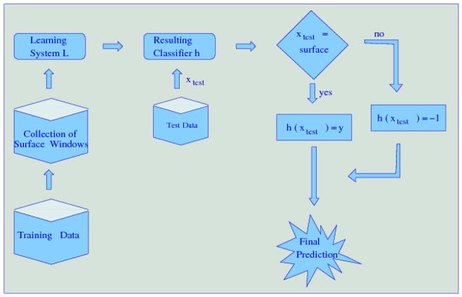
To take advantage of the structural information, we developed a two-stage classifier, called Struct-NB: in the first stage, the windows that correspond to the surface target residues (i.e., target residues that are on the surface) are separated from those that correspond to the non-surface target residues; in the second stage, if the target residue is on the surface, the classifier returns a probability that this residue is an interface residue given the sequence or structural features as input to the classifier; otherwise, if the target residue is not on the surface, the classifier assigns this residue as a non-interface residue (see Figure 1). One important advantage of this model is that it allows the use of existing machine learning methods. In this study, we used Naïve Bayes classifiers.

Figure 1.

Struct-NB: a two-stage classifier that integrates domain knowledge (i.e., structural information) to improve classification performance. In the first stage, the windows corresponding to each residue are split according to their surface/non-surface label. In the second stage, if the current residue is a surface residue, the classifier returns a probability that this residue is an interface residue; otherwise, the classifier assigns this residue to be a non-interface residue.

2.7.4 Ensemble of Naïve Bayes classifiers

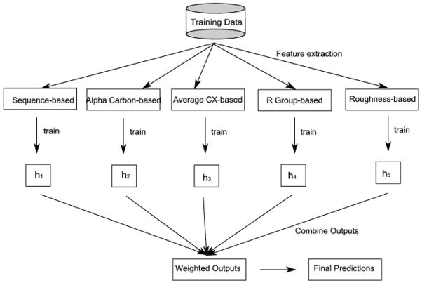
An ensemble of Naïve Bayes classifiers is a collection of Naïve Bayes classifiers, each trained on a different feature representation of the training data (see Figure 2). The prediction of the ensemble of Naïve Bayes classifiers is computed from the predictions of the individual Naïve Bayes classifiers. That is, during classification, for a new instance x_test, each individual Naïve Bayes classifier in the collection returns a probability P_j(y_i|x_test), that x_test belongs to a particular class y_i, where j = 1; · · ·, n, and n is the number of Naïve Bayes classifiers in the collection. The ensemble estimated probability, P_Ens(y_i|x_test) is obtained by:

$$P_{\mathit{Ens}}\left(y_i\mid {\mathbf{x}}_{\mathit{test}}\right)=\frac{1}{n}\sum _j^n{P}_j\left(y_i\mid {\mathbf{x}}_{\mathit{test}}\right)$$

Figure 2.

A schematic of the Ensemble classifier used for combining information from the multiple feature representations. As can be seen from the figure, a classifier is trained using sequence and structural features. The prediction of the ensemble is then obtained from the predictions of individual classifiers.

In our experiments, we trained 5 Naïve Bayes classifiers (n = 5), one for each feature representation: sequence-based, alphacarbon-based, averagecx-based, rgroup-based, and roughness-based feature representations, respectively.

2.8 Performance Evaluation of Classifiers

Standard approaches to assessing the performance of classifiers rely on k-fold cross-validation wherein a dataset is partitioned into k disjoint subsets (folds). The performance measure of interest is estimated by averaging the measured performance of the classifier on k runs of a cross-validation experiment, each using a different choice of the k − 1 subsets for training and the remaining subset for testing the classifier. In our experiments, we used sequence-based (as opposed to window-based) cross-validation, a procedure that guarantees that training and test sets are disjoint at the sequence level [Caragea et al., 2007]. To assess the performance of our classifiers we reported the following measures described in [Baldi et al., 2000]: Sensitivity+, and Specificity+, Receiver Operating Characteristic (ROC) curve, and Area Under the ROC Curve (AUC). If we denote true positives, false negatives, false positives, and true negatives by TP, FN, FP, and TN respectively, then the Sensitivity+ and the Specificity+ can be defined as follows:

$$\text{Sens}+=\frac{TP}{TP+FN}$$ (1)

$$\text{Spec}+=\frac{TP}{TP+FP}$$ (2)

The ROC curve plots the proportion of correctly classified positive examples, True Positive Rate (TPR) as a function of the proportion of incorrectly classified negative examples, False Positive Rate (FPR) for different classification thresholds. In comparing two different classifiers using ROC curves, for the same False Positive Rate, the classifier with higher True Positive Rate gives better performance measures. Each point on the ROC curve represents a classification threshold θ and corresponds to particular values of TPR and FPR.

To evaluate how good a classifier is at discriminating between the positive and negative examples, we also report the AUC on the test set, which represents the probability of correct classification [Baldi et al., 2000]. That is, an AUC of 0.5 indicates a random discrimination between positives and negatives (random classifier), while an AUC of 1 indicates a perfect discrimination (very good classifier).

3 Results

Now we proceed to explore the questions: Do protein-RNA interfaces differ from non-interfaces in terms of their structural features? Do the structural features vary with the type of bound RNA? How useful can structural features be to reliably predicting protein-RNA interface residues?

3.1 CX Protrusion Index

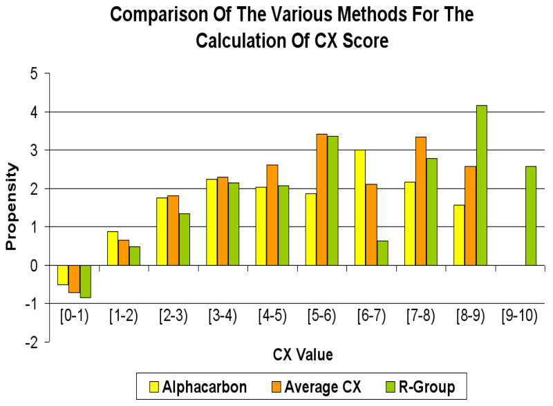
Figure 3 shows the relative CX score propensities of the interface residues, based on three different calculations of CX score for each residue: the average of the CX scores for all atoms (averagecx); use the average of the CX scores atoms in the R-group only (rgroup); or the CX score for the alpha carbon atom as the score for the corresponding residue (alphacarbon). The figure shows that averaging the CX score across all atoms in the residue produces similar results to averaging across the R-group atoms alone.

Figure 3.

Comparison of various methods to obtain CX values for residues on the protein surface. The figure shows that averaging the CX score across all atoms in the residue produces similar results to averaging across the R-group atoms alone.

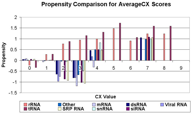
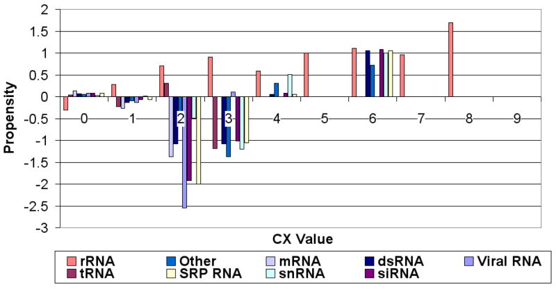
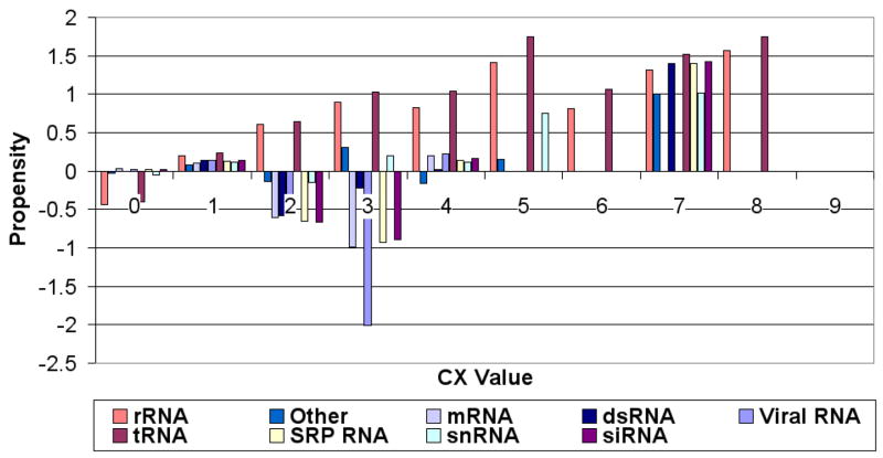
Figures 4, 5 and 6 (respectively) show the residue propensities based on the types of the bound RNA using the averagecx, alphacarbon and rgroup methods respectively. The observed CX value residue propensities of interfaces involving different types of RNA appear to be sensitive to the method used to calculate the CX values.

Figure 4.

Propensity scores for CX values (Y-axis) calculated using the averagecx for different ranges of CX values (X-axis). Propensities for CX values 0–4 tend to vary across different RNA types as compared to propensities for higher CX scores. Different colors correspond to different RNA types.

Figure 5.

Propensity scores for CX values (Y-axis) calculated using the alphacarbon for different ranges of CX values (X-axis). Different colors correspond to different RNA types.

Figure 6.

Propensity scores for CX values (Y-axis) calculated using the rgroup for different ranges of CX values (X-axis). Different colors correspond to different RNA types.

ANOVA analysis for the alphacarbon method (ANOVA p-value = 0.056, cutoff = 0.05) shows that tRNA and mRNA cluster together with variances around 0.2. SnRNA, rRNA, dsRNA and “other” cluster together with variances around 0.3. Finally, siRNA, SRP RNA and Viral RNA cluster together with variances around 0.65. ANOVA analysis for the averagecx method (ANOVA p-value = 0.00001, cutoff = 0.05) shows that Viral RNA, mRNA, “other”, and snRNA cluster together with variances around 0.2. DsRNA, rRNA siRNA and SRP RNA cluster together with variance around 0.35 and tRNA is the only RNA type with variance around 0.5. The results of ANOVA analysis for the rgroup method (ANOVA p-value = 0.0002, cutoff = 0.05) are similar to those of averagecx with mRNA, snRNA and “other” clustering together with variances around 0.13, whereas dsRNA, SRP RNA, siRNA, rRNA and Viral RNA cluster together with variances around 0.37. Finally, the tRNA group is isolated with a variance of 0.5.

Regardless of the method used to calculate the CX scores, we can observe some general trends: The rRNA and tRNA propensities are always negative at CX score range [0,1) and have an increasing propensity as the CX scores increase. However, all other types of RNA (mRNA, snRNA...etc) tend to have low (negative) propensity values from [0,4), and the propensities for all types then tend to rise after CX range [4,5). One interesting exception is the score range [0,1), which tends to have slightly positive (albeit very small) interface propensities in the case of RNAs other than tRNA and rRNA, suggesting that in protein-RNA interfaces containing such RNAs non-protruding residues can be interface residues. The CX value residue propensities of interface residues bound to Viral RNAs and rRNAs appear to differ significantly from that of residues that bind to other types of RNAs figures 4, 5 and 6.

3.2 Roughness Value

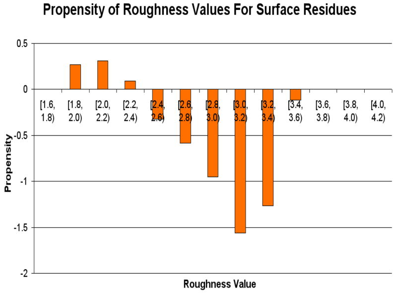
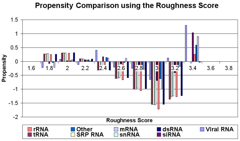
Figure 7 shows the propensities for the roughness score. Residues with rough surfaces are preferred in protein-RNA interfaces. Figure 8 shows the distribution of the propensities for each roughness score range classified by the type of RNA. The figure indicates that, unlike the CX scores, the roughness scores do not vary significantly among the different types of RNA at each score range as all RNA types behave almost identically for each roughness score range (ANOVA p-value = 0.32 with cutoff 0.05). Using the variances calculated by ANOVA, tRNA, SRP RNA, snRNA, rRNA and dsRNA seem to cluster well with each other (all have variances close to 0.2). The remaining RNA types (Viral RNA, siRNA, mRNA and “other”) have variances around 0.1.

Figure 7.

The propensity values for various roughness scores on the surface residues.

Figure 8.

Propensity scores for roughness values classified by RNA type. Roughness propensity is similar across different types of RNA interfaces

3.3 Protein-RNA Interface Prediction using Struct-NB

The main result of our study using machine learning approaches is that the Struct-NB classifiers described here outperform sequence-based Naïve Bayes and structural-based Gaussian Naïve Bayes classifiers on the problem of predicting RNA-binding sites in protein sequences.

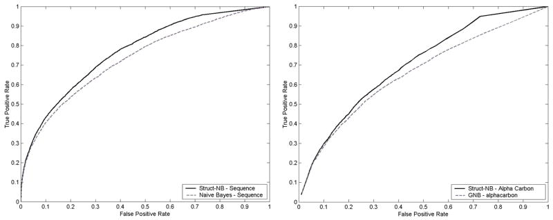
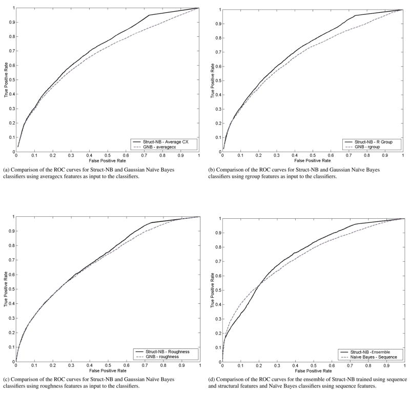
We trained Struct-NB classifiers, that take into account structural information, using sequence and structural features, Naïve Bayes using sequence features, and Gaussian Naïve Bayes using structural features. We compared the ROC curves of sequence-based Naïve Bayes and structural-based Gaussian Naïve Bayes with those of Struct-NB classifiers on the 147 protein-RNA dataset. The ROC curves show the tradeoff between true positive rate and false positive rate over their entire range of possible values. Hence, it is more informative to compare the ROC curves than to compare the performance of the classifiers for a particular choice of the tradeoff (which corresponds to a specific point θ on the ROC curve). We found that the ROC curve for Struct-NB dominates the ROC curve for sequence-based Naïve Bayes and structural-based Gaussian Naïve Bayes. That is, for any choice of false positive rate, Struct-NB offers a higher true positive rate than both sequence-based Naïve Bayes and structural-based Gaussian Naïve Bayes (Figures 10a,10b,11a,11b and 11c). In Figure 11d we compare the performance of the ensemble of Struct-NB classifiers, that combines the predictions of individual Struct-NB classifiers trained using sequence and structural features, with that of the Naïve Bayes using sequence features. As can be seen, for values of the false positive rate higher than 0.2, the ensemble of Struct-NB has a higher Sensitivity than that of the sequence-based Naïve Bayes.

Figure 10.

Comparison of Struct-NB and Gaussian Naïve Bayes classifiers utilizing sequence (10a) and Alphacarbon (10b) as input to the classifiers.

Figure 11.

Comparison of Struct-NB and Gaussian Naïve Bayes classifiers utilizing averagecx (11a), rgroup (11b) and roughness (11c) as input to the classifiers. Figure 11d shows a comparison of the ensemble Struct-NB classifier trained using sequence and structural features with a Naïve Bayes classifier using sequence features.

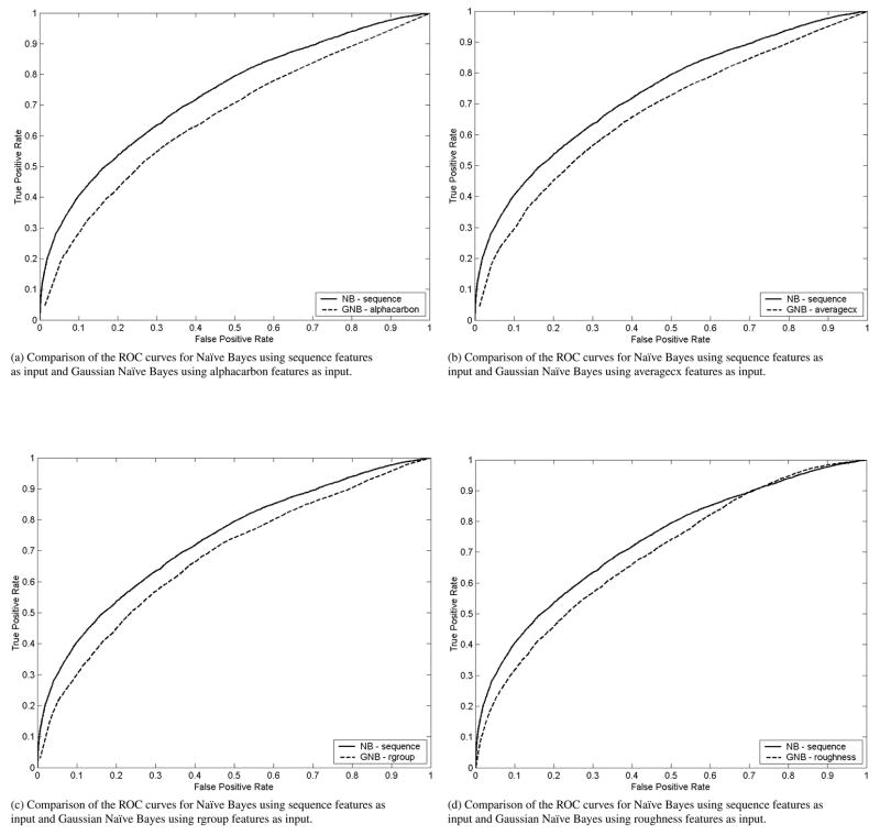
In addition, we compared the ROC curves of Naïve Bayes using sequence features with that of Gaussian Naïve Bayes using structural features. We found that while the ROC curves for sequence-based Naïve Bayes dominates the ROC curves for structural-based Gaussian Naïve Bayes (see Figures 12a,12b,12c,12d), the structural-based Gaussian Naïve Bayes has a higher sensitivity than sequence-based Naïve Bayes and sequence-based Naïve Bayes has a higher specificity than structural-based Gaussian Naïve Bayes.

Figure 12.

Comparison of Gaussian Naïve Bayes classifiers utilizing alphacarbon (12a), averagecx (12b), rgroup (12c) and roughness (12d) as input to the classifiers with a Naïve Bayes classifier trained using sequence features.

In Table 2, we show a comparison of the performance statistics for the Gaussian Naïve Bayes using alphacarbon, averagecx, rgroup, roughness features respectively, the Naïve Bayes using sequence features, and the ensemble of Struct-NB. The statistics are reported for the same threshold θ = 0.5 on the ROC curves. As can be seen, sequence-based Naïve Bayes achieves Sensitivity+ = 0.246, Specificity+ = 0.65, and AUC = 0.736, structural-based Gaussian Naïve Bayes using roughness features achieves Sensitivity+ = 0.349, Specificity+ = 0.469, and AUC = 0.696, and the ensemble of Struct-NB achieves Sensitivity+ = 0.359, Specificity+ = 0.443, and AUC = 0.752. Therefore, in applications that require a higher sensitivity, a better choice is to use structural feature as input to the Naïve Bayes classifiers. This is visually shown in Figure 9.

Table 2.

A comparison of AUC, Sensitivity+, and Specificity+ for Gaussian Naïve Bayes classifier using alphacarbon, averagecx, rgroup, and roughness features respectively, Naïve Bayes using sequence features, and Struct-NB-Ensemble that combines sequence and structural features. The values are reported for the same threshold θ = 0.5 on the ROC curve.

Name	AUC	Sens+	Spec+
NB-AC	0.658	0.368	0.36
NB-ACX	0.672	0.397	0.366
NB-RG	0.679	0.403	0.367
NB-RN	0.696	0.469	0.349
NB-Seq	0.736	0.246	0.65
Struct-NB-Ensemble	0.752	0.359	0.443

Figure 9.

Comparison of predictions on 2AW4 chain 0 from the Struct-NB using roughness features, Gaussian Naïve Bayes using roughness features, and Naïve Bayes using sequence features. The second line shows the actual labels.

4 Summary and Discussion

We have analyzed a non-redundant dataset of protein-RNA interfaces in terms of two structural properties of amino acid residues, namely, CX score and roughness. The results of our analysis show that:

• Amino acid residues in protein-RNA interfaces tend to be more protruding (as measured by CX values) compared with surface residues.

• Amino acid residues in protein-RNA interface tend to have more rough surfaces compared with surface residues.

• Considering the location of the residue in the protein structure (surface vs non-surface) improves the performance of both sequence-based and structure-based classifiers.

• The structural features (CX and roughness values) can be used to classify protein-RNA interfaces using an ensemble approach. The resulting classifier is able to identify protein-RNA interfaces at a higher sensitivity compared to a sequence-based classifier at the same θ threshold.

It is possible that the general trends observed across all RNA types is biased by rRNA-binding proteins, which make up over half of the protein-RNA complexes in PDB. One way to determine whether this is indeed the case is to repeat the protein-RNA interface analysis separately for each RNA-type. Also of concern is the relatively small size of the RB147 dataset protein-RNA dataset. Terribilini et al. [Terribilini et al., 2007] have noted that PDB included only 198 proteinnucleic acid complexes in 1996, but by April 2007, this number had grown to 1,734, of which 529 were proteinRNA complexes. The resulting availability of larger and more diverse datasets can be expected to significantly improve the quality and quantity of data available for performing the analysis of the sort reported here. Work in progress is aimed at:

• Assembling a comprehensive of protein-RNA interface database (PRIDB), and associated services for querying, analysis, and visualization of protein-RNA interfaces.

• Developing machine learning approaches for reliable identification of putative RNA-binding residues in proteins that improve upon the state-of-the-art sequence-based methods [Terribilini et al., 2006b] by taking advantage of structural and molecular dynamics simulations.

• Analysis of sequence and structural properties of protein-binding residues in RNA and the development of machine learning approaches for reliable identification of putative protein-binding RNA residues.

• Characterization of the sequence and structural correlates of protein-RNA interfaces and the similarities and differences among different types of protein-RNA interfaces, and between protein-protein, protein-DNA, and protein-RNA interfaces.

References

- Baldi P, Brunak S, Chauvin Y, Andersen C, Nielsen H. Assessing the accuracy of prediction algorithms for classification: an overview. Bioinformatics. 2000;16(5):412–424. doi: 10.1093/bioinformatics/16.5.412. [DOI] [PubMed] [Google Scholar]
- Bechara E, Davidovic L, Melko M, Bensaid M, Tremblay S, Grosgeorge J, Khandjian EW, Lalli E, Bardoni B. Fragile x related protein 1 isoforms differentially modulate the affinity of fragile x mental retardation protein for g-quartet rna structure. Nucleic Acids Research. 2007;35:299–306. doi: 10.1093/nar/gkl1021. [DOI] [PMC free article] [PubMed] [Google Scholar]
- Berman H, Westbrook J, Feng Z, et al. The protein data bank. Nucleic Acids Res. 2000;28:235–242. doi: 10.1093/nar/28.1.235. [DOI] [PMC free article] [PubMed] [Google Scholar]
- Caragea C, Sinapov J, Silvescu A, Dobbs D, Honavar V. Glycosylation site prediction using ensembles of support vector machine classifiers. BMC Bioinformatics. 2007;8(438) doi: 10.1186/1471-2105-8-438. [DOI] [PMC free article] [PubMed] [Google Scholar]
- Chen Y, Varani G. Protein families and rna recognition. FEBS Journal. 2005;272(9):2088–2097. doi: 10.1111/j.1742-4658.2005.04650.x. [DOI] [PubMed] [Google Scholar]
- Connolly ML. Measurement of protein surface shape by solid angles. Journal of Molecular Graphics. 1986;4(1):3–6. [Google Scholar]
- Connolly ML. The molecular surface package. J Mol Graph. 1993;11(2):139–41. doi: 10.1016/0263-7855(93)87010-3. [DOI] [PubMed] [Google Scholar]
- Dietterich TG. Machine learning for sequential data: A review. Structural, Syntactic, and Statistical Pattern Recognition; Lecture Notes in Computer Science. 2002;2396:15–30. [Google Scholar]
- Ellis J, Broom M, Jones S. Protein-rna interactions: structural analysis and functional classes. Proteins. 2007;66(4):903–11. doi: 10.1002/prot.21211. [DOI] [PubMed] [Google Scholar]
- Freed EO, Mouland AJ. The cell biology of hiv-1 and other retroviruses. Retrovirology. 2006;3(77) doi: 10.1186/1742-4690-3-77. [DOI] [PMC free article] [PubMed] [Google Scholar]
- Jeong E, Chung I-F, Miyano S. A neural network method for identification of rna-interacting residues in protein. Genome Informatics. 2004;15(1):105–116. [PubMed] [Google Scholar]
- Jeong E, Miyano S. A weighted profile method for protein-rna interaction prediction. Trans On Comput Syst Biol. 2006;IV:123–139. [Google Scholar]
- Jones S, Daley DTA, Luscombe NM, Berman HM, Thornton JM. Protein-rna interactions: a structural analysis. Nucleic Acids Research. 2001;29(4):943–954. doi: 10.1093/nar/29.4.943. [DOI] [PMC free article] [PubMed] [Google Scholar]
- Jurica MS, Moore MJ. Pre-mrna splicing: awash in a sea of proteins. Mol Cell. 2003;12:5–14. doi: 10.1016/s1097-2765(03)00270-3. [DOI] [PubMed] [Google Scholar]
- Lee B, Richards FM. The interpretation of protein structures: Estimation of static accessibility. J Mol Biol. 1971;55:379–400. doi: 10.1016/0022-2836(71)90324-x. [DOI] [PubMed] [Google Scholar]
- Lejeune D, Delsaux N, Charloteaux B, Thomas A, Brasseur R. Protein-nucleic acid recognition: statistical analysis of atomic interactions and influence of dna structure. Proteins. 2005;61(2):258–71. doi: 10.1002/prot.20607. [DOI] [PubMed] [Google Scholar]
- Lewis M, Rees D. Fractal surfaces of proteins. Science. 1985;230(4730):1163–1165. doi: 10.1126/science.4071040. [DOI] [PubMed] [Google Scholar]
- M T, E W. Statistical analysis of atomic contacts at rna-protein interfaces. J Mol Recognit. 2001;14(4):199–214. doi: 10.1002/jmr.534. [DOI] [PubMed] [Google Scholar]
- Mitchell T. Machine Learning. McGraw-Hill; Boston, MA: 1997. [Google Scholar]
- Mitchell T, Hutchinson R, Niculescu RF, Pereira Wang X, Just M, Newman S. Learning to decode cognitive states from brain images. Machine Learning Journal. 2004;57:145–175. [Google Scholar]
- Moore MJ. From birth to death: the complex lives of eukaryotic mrnas. Science. 2005;309:15141518. doi: 10.1126/science.1111443. [DOI] [PubMed] [Google Scholar]
- Noller HF. Rna structure: reading the ribosome. Science. 2005;309:15081514. doi: 10.1126/science.1111771. [DOI] [PubMed] [Google Scholar]
- Pintar A, Carugo O, Pongor S. Cx, an algorithm that identifies protruding atoms in proteins. Bioinformatics. 2002;18(7):980–4. doi: 10.1093/bioinformatics/18.7.980. [DOI] [PubMed] [Google Scholar]
- Terribilini M, Lee J-H, Yan C, Jernigan RL, Carpenter S, Honavar V, Dobbs D. Identifying interaction sites in ”recalcitrant” proteins: Predicted protein and rna binding sites in rev proteins of hiv-1 and eiav agree with experimental data. Pacific Symposium on Biocomputing. 2006a;11:415–426. [PMC free article] [PubMed] [Google Scholar]
- Terribilini M, Lee J-H, Yan C, Jernigan RL, Honavar V, Dobbs D. Prediction of rna binding sites in proteins from amino acid sequence. Bioinformatics. 2006b;12:1450–1462. doi: 10.1261/rna.2197306. [DOI] [PMC free article] [PubMed] [Google Scholar]
- Terribilini M, Sander JD, Lee J-H, Zaback P, Jernigan RL, Honavar V, Dobbs D. Rnabindr: a server for analyzing and predicting rna-binding sites in proteins. Nucleic Acids Research. 2007;35(2):1–7. doi: 10.1093/nar/gkm294. [DOI] [PMC free article] [PubMed] [Google Scholar]
- Towfic F, Gemperline DC, Caragea C, Wu F, Dobbs D, Caragea C. Structural characterization of rna-binding sites of proteins: Preliminary results. Computational Structural Bioinformatics Workshop 2007 [Google Scholar]
- Wu F, Towfic F, Dobbs D, Honavar V. Analysis of protein protein dimeric interfaces. IEEE International Conference on Bioinformatics and Biomedicine proceedings 2007 [Google Scholar]