Abstract
Selective sweeps can increase genetic differentiation among populations and cause allele frequency spectra to depart from the expectation under neutrality. We present a likelihood method for detecting selective sweeps that involves jointly modeling the multilocus allele frequency differentiation between two populations. We use Brownian motion to model genetic drift under neutrality, and a deterministic model to approximate the effect of a selective sweep on single nucleotide polymorphisms (SNPs) in the vicinity. We test the method with extensive simulated data, and demonstrate that in some scenarios the method provides higher power than previously reported approaches to detect selective sweeps, and can provide surprisingly good localization of the position of a selected allele. A strength of our technique is that it uses allele frequency differentiation between populations, which is much more robust to ascertainment bias in SNP discovery than methods based on the allele frequency spectrum. We apply this method to compare continentally diverse populations, as well as Northern and Southern Europeans. Our analysis identifies a list of loci as candidate targets of selection, including well-known selected loci and new regions that have not been highlighted by previous scans for selection.
A selective sweep alters the allele frequencies of single nucleotide polymorphisms (SNPs) in the vicinity of the selected allele, and thus causes a distorted pattern of genetic variation that can be useful for detecting selection. The scans for selection that have sought to detect such signals have largely been based on searching for a distortion in the allele frequency spectrum or haplotype structure in a single population (Tajima 1989; Fu and Li 1993; Fay and Wu 2000; Sabeti et al. 2002; Nielsen et al. 2005; Voight et al. 2006; for review, see Akey 2009).
The first scans for selection that took advantage of differentiation across populations focused on single-marker Fst (Lewontin and Krakauer 1973; Akey et al. 2002). However, this statistic is highly variable over loci under neutrality (Weir et al. 2005), making it difficult to find an Fst statistic that is genome-wide significant unless the signal-to-noise ratio is high as in closely related populations, such as Northern and Southern Europeans (Price et al. 2008). To address this limitation, Weir et al. (2005) and Oleksyk et al. (2008) proposed studying the average of Fst over multilocus windows. However, these methods do not take advantage of the nontrivial way that Fst depends on the allele frequency of the SNPs before selection.
Another approach to identifying signals of selection through population comparison is the cross-population extended haplotype heterozygosity test (XP-EHH), which was designed to detect ongoing or nearly fixed selective sweeps by comparing haplotypes from two populations. (Sabeti et al. 2007; Tang et al. 2007). However, since this method relies on linkage disequilibrium (LD), which breaks down quickly over time, it provides weak power to detect historical sweeps that are “ancient” and ended up to several thousand generations ago.
Selection has also been identified using methods that model the allele frequency spectrum to search for signals of selection. Williamson et al. (2007), building on Nielsen et al. (2005), applied a multiple-locus composite likelihood ratio method (CLR) to screen for selection in two populations. However, they did not take advantage of the characteristic differences in allele frequencies across two populations that are expected to arise in the case of natural selection. Nielsen et al. (2009) recently introduced a new method that is able to take advantage of allele frequency differences across populations by modeling the neutral two-dimensional frequency spectrum using genome-wide data and searching for locus-specific outliers. However, a limitation is that unlike the single-population CLR method, this method does not model the joint allele frequency spectrum under selection, and thus cannot support a likelihood ratio test. Moreover, all of these methods are very sensitive to SNP ascertainment bias.
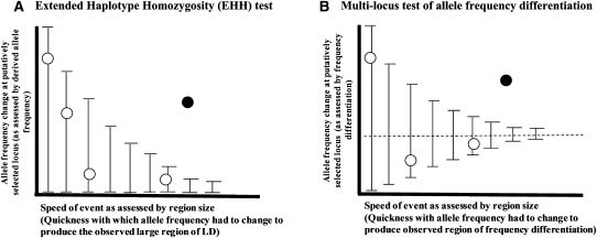
We present a new statistical method for detecting selective sweeps based on multilocus allele frequency differentiation between two populations, which achieves multiple advantages over these existing methods. Our method is best understood in analogy to the extended haplotype homozygosity (EHH) test (Sabeti et al. 2002) (Fig. 1). In the EHH test, one searches for alleles that are of substantial frequency, suggesting that they arose a long time ago, but which are, in fact, too young to be consistent with neutrality (the age of the allele can be measured based on the extent of LD around it). In our method, we search for regions in the genome, where the change in allele frequency at the locus occurred too quickly (as assessed by the size of the affected region) to be due to random drift. The details of this method are presented below.
Figure 1.
An analogy between the extended haplotype homozygosity (EHH) test and a multimarker test of unusual allele frequency differentiation. (A) In the EHH test, one searches for sites where the change in allele frequency since a putative selection event began (as assessed by its derived allele frequency) occurred too quickly (as assessed by the extent of LD around the tested allele) due to random genetic drift. The open circles show the expectation under neutrality, while the filled circles shows a selection signal (adapted from Fig. 3 of Sabeti et al. 2002). (B) In the multilocus test of allele frequency differentiation (XP-CLR) the idea is to search for regions in the genome where the change in allele frequency at the locus occurred too quickly (as assessed by the size of the affected region) due to random drift. A large region with moderate differentiation can easily stand out as genome-wide significant (filled circle).
Results
Parametric method
Suppose that we are investigating the allele frequencies of a neutral SNP in two populations with allele frequencies p1 and p2, respectively. The allele frequencies can be modeled by a Wiener process from a common allele frequency p0 in the ancestral population (Nicholson et al. 2002). That is, p1 and p2 follow a normal distribution:
with σ2 ≈ ωp0(1 − p0). Here, ω contains all information concerning the population histories since the split time, including the genetic drift times and bottleneck events. This is a good approximation when σ is small. The Wiener process is time reversible, and thus we can approximate the whole process by assuming that the frequency starts from p2 in population 2, evolves backward in time to the split time, and then evolves forward to p1. Thus, by replacing p0 in Equation 1 with p2, we obtain the distribution of allele frequency in population 1 (“objective” population) as a function of that in population 2 (“reference” population).
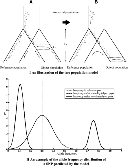
To model the effect of a selective sweep at a selected allele A in population 1, we study the expected distortion in the allele frequency of a neutral allele B in the vicinity. For simplicity of modeling, we assume that selection completed at the current generation (Fig. 2, top).
Figure 2.
(Top panel) Illustration of the two-population model. (A) The two populations split at divergence time Td. The dotted lines represent the historical frequencies of an allele in the two populations; the dashed lines represent the increase of its allele frequency during the selection phase due to hitchhiking with a nearby advantageous allele. (B) Illustration of the modeling procedure. Starting from the observed allele frequency of a SNP in the reference population, the model predicts the allele frequency distributions under neutrality or selection in the object population. (Bottom panel) An example of the allele frequency distribution of a SNP near a putatively selected allele in the object population under selection (Equation 4, solid line) and neutrality (Equation 1, dashed line). The vertical dotted line represents the allele frequency of the SNP in the reference population (p2 = 0.3). The ratio r/s of genetic distance between the SNP and the advantage allele mutant divided by selection intensity is 0.05. The two populations are both assumed to have effective sizes 10,000. The divergence time ω is set to be 0.04.
Given the allele frequency p2 of allele B in population 2, we assume that the allele frequency p1* in the objective population before selection follows a normal distribution as in Equation 1. To model the joint effect of selection and recombination on the distribution of p1 after selection, we follow Maynard Smith and Haigh (1974), who used a continuous approximation and a logistic sweep model to derive the result that if the allele is linked to the selected allele A, its frequency is expected to be increased to 1 − c + cp1* after selection. Otherwise, if it is linked to the other allele a, its allele frequency is expected to be reduced to cp1*, where
 |
Here, r is the recombination fraction between the selected allele A and the neutral allele B, s is the selection coefficient, and q0 is the initial allele frequency of A in population 1. Durrett and Schweinsberg (2004) showed that for a wide range of r/s, Equation 2 can be approximated by:
By applying a linear transformation following Fay and Wu (2000), we can derive the distribution of allele frequencies after a selective sweep as:
 |
where I[a,b](x) is 1 on the interval [a,b], and 0 otherwise. Here, p2 is the allele frequency observed in population 2, and c is defined as before. When s→0 or r > s, the distribution converges to Equation 1. Figure 2, bottom, shows an example of the predicted allele frequency distribution, which has a nontrivial shape that we model to increase power to detect selection.
So far, we have focused on predicting the allele frequency distribution at a single marker. We now generalize to the analysis of extended regions, where the allele frequencies of multiple contiguous markers are distorted from the prediction under neutrality, and where the allele frequency differences between two populations have an expected “spatial” pattern as a function of genetic distance to the selected allele. Analytic derivation of the joint distribution of allele frequency at multiple markers is challenging due to the complex correlations among sites. We therefore use a composite likelihood approach in which we multiply the marginal likelihood function of the k SNPs:
 |
where r stands for {r1, r2, …, rk}, n is the sample size, and mi is the count of allele B at locus i. We define a statistic similar to the likelihood ratio of the alternative over the null hypothesis.
Although we choose a sliding window of size k in the formalization of the likelihood function, the method does not depend on the choice of window size when the window is sufficiently large. When r > s, the marginal likelihood for that SNP locus is identical under the two hypotheses.
A shortcoming of composite likelihood methods is that the correlation of marginal likelihood terms in the composite likelihood function is ignored (Lindsay 1988). Thus, these methods overestimate the amount of information that is available in the data, which can result in false-positive signals of selection. To partially control for this problem, we assigned weights to each of the marginal likelihood functions in proportion to their statistical independence of all of the others. We implemented this idea by studying the correlation (pairwise LD) of SNPs in the reference population, down-weighting SNPs that are in LD. We weighted SNPs i according to:
 |
where corr(i,j) is the pairwise correlation coefficient of two SNPs, and I(·) is an indicator function equal to 1 if corr(i,j) is above some prechosen cut-off level, and 0 otherwise. An intuitive explanation is that when several SNPs are in perfect LD or highly correlated, they provide redundant information and their contribution to the likelihood function should be down-weighted or even treated as a single piece of information. In practice, we found that this weighting scheme is useful for reducing false-positive signals. We note that this is an innovation of our approach compared with other composite likelihood methods for detecting selection. When analyzing data from only a single population, it is difficult to distinguish the autocorrelation among SNPs that is expected under neutrality from that caused by selection. However, when two populations are compared, one can use LD in the reference population to perform an appropriate SNP weighting that is not affected by selection.
Properties of the XP-CLR test when applied to simulated data
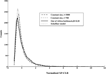
To investigate the statistical properties of our method (We name it “the cross-population composite likelihood ratio test”, or XP-CLR), we carried out simulations with a range of parameters. We first investigated the null distributions of XP-CLR scores for different demographic models. Four historical scenarios were considered (Supplemental material), and samples were generated by coalescent simulations. We found that the mean and variance of the XP-CLR scores for the comparison of African to non-African populations were larger than those of the comparisons of closely related populations. However, the distributions had the same shape. After subtracting the mean and dividing by the standard deviation, the distribution of normalized XP-CLR scores closely matched regardless of the demography we analyzed (Fig. 3). Based on this, we hypothesized that the normalized XP-CLR scores might be robust to variation in demographic models, which is a valuable property of our test, since current models of human demographic history are, of course, imperfect approximations to the truth. The robustness suggests that we might even be able to interpret XP-CLR scores formally in terms of P-values. In this study, to be conservative, we do not assign P-values, but instead follow Voight et al. (2006) and Pickrell et al. (2009), and rank-order scores across the genome.
Figure 3.
The empirical distributions of XP-CLR scores normalized by their means and variances under a variety of demographic scenarios, showing the robustness to demographic histories.
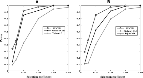
We explored the power of this method to detect both recent sweeps and “ancient sweeps,” by which we mean any sweeps that started after the divergence of two populations and ended in the past dating back as far as several thousand generations ago. We set the fixation time to be 1000 generations ago for “ancient sweeps,” and the current generation for “recent sweeps.” To match the density of SNPs in typical modern genotyping data, we simulated about one SNP per 3 kb. Two frequency spectrum-based methods, Nielsen et al. (2005)'s composite likelihood ratio (CLR) method and Tajima's D test (Tajima 1989), were also applied to the simulated data. We used a threshold for statistical significance such that the false-positive rate was 0.01 for all tests. The statistical cutoffs were determined by neutral simulations with the ms software (Hudson 2002) (Methods), and the proportion of significant results was used to determine the power for detecting selection. Our simulations show that the power of XP-CLR exceeds Tajima's D and CLR for a range of selection intensities (Fig. 4).
Figure 4.
The proportions of significant results for three tests of selection, as assessed by simulations for recent sweeps (A) and ancient sweeps (B). (XP-CLR) the method developed in this study; (Tajima D) Tajima's D test on the data from the object population; (Nielsen CLR) the method developed by Nielsen et al. (2005). Simulations were carried out with constant population sizes of 10,000 and population divergence time of 3000 generations with the code p2S (detailed in Methods). The false-positive rate is chosen to be 0.01. “Ancient” refers to the scenarios in which selection stops at 1000 generations ago; “recent” refers to selection stopping at the current generation.
We further tested the method's accuracy in inferring the location of the selected allele. For each of the simulated data sets, we generated a sample of 100 haplotypes for a 500-kb region, and positioned the advantageous mutant in the middle of the region. The inferred positions of the advantageous mutants from our method are illustrated in Supplemental Figure S1. Most inferred locations are within a 30-kb distance from the true location for selection intensities of 0.005. The precision of localization is, of course, a function of the selection intensity.
Robustness to ascertainment bias
Current SNP arrays use markers that were selected in complex ways, which causes distortions of the shape of the allele frequency distribution, or “ascertainment bias” (Nielsen et al. 2004; Clark et al. 2005). This can bias tests of selection based on the allele frequency spectrum, such as the CLR test and G2D (Nielsen et al. 2009). While these effects can be ameliorated by modeling the SNP ascertainment scheme, this approach requires precise knowledge of how SNPs were chosen, which is often not known (Clark et al. 2005).
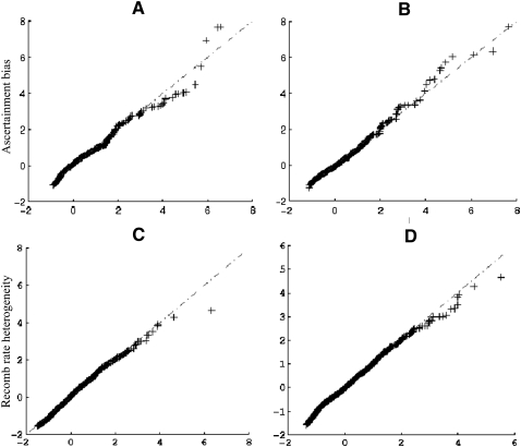
The XP-CLR test is based on allele frequency differentiation across populations, which is not as affected by ascertainment bias. To test how XP-CLR performs in the face of ascertainment bias, we simulated two types of bias: (1) We restricted to SNPs with a frequency >5% in the reference population, and (2) we restricted to SNPs that were polymorphic in a pilot sample of two chromosomes from each of the two populations. Figure 5, A and B, and Supplemental Figure S2, A and B, demonstrate that the normalized XP-CLR scores under the two ascertainment schemes follow almost identical distributions as they do without ascertainment bias.
Figure 5.
(A,B) A comparison of XP-CLR scores calculated from simulations of an ascertainment bias scheme in which SNPs are discovered in a pilot sample that included two chromosomes from each population. (A) Constant population size model with divergence time of T = 700 generations ago. (B) Constant population size model with divergence time of T = 3000 generations ago. Note that the XP-CLR scores in the figures were normalized. (C,D) A comparison of XP-CLR scores calculated from simulations of models assuming constant recombination rates with those including recombination hotspots or misspecified recombination rates. (C) The recombination hotspot model. (D) Estimated recombination rate is one-fourth of the true recombination rates. XP-CLR scores were normalized before this analysis.
Robustness to recombination rate heterogeneity
Recombination rates are known to vary dramatically at fine-scales (Myers et al. 2005). To explore the robustness of the XP-CLR method to uncertainty in the local recombination rate, we performed neutral simulations of 500-kb regions with an overall recombination rate of 1.25 cM/Mb, and simulated recombination hotspots of 2 kb in size that were spaced every 25 kb (the within-hotspot recombination rate was t times higher than the background, with t exponentially distributed with mean equal to 6). We also explored the effect of systematically misestimating a uniformly distributed recombination rate by 1/2, 1/4, two-, and fourfold. Figure 5, C and D, and Supplemental Figure S2, C and D, show that recombination rate uncertainty does not cause substantial distortions in the expected XP-CLR statistic.
Analysis of real data
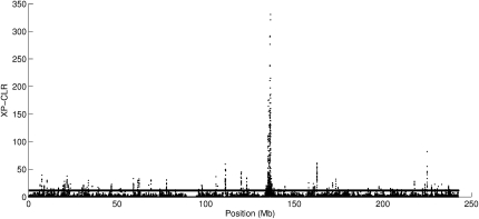
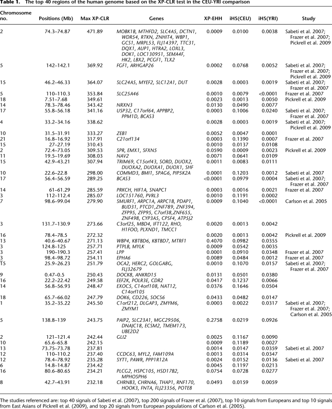
We applied XP-CLR to comparisons of West African, North European, and East Asian samples from HapMap Phase II, and to Northern and Southern European ancestry samples from POPRES (Nelsen et al. 2008) (Supplemental Figs. S3–S6). The strongest XP-CLR score in the comparison of Northern and Southern European is on chromosome 2, near the lactase gene (LCT) (Fig. 6). Table 1 and Supplemental Tables S1 and S2 list the 40 genomic regions with the strongest evidence for sweeps from the comparison of different population pairs, along with the genome-wide ranks of XP-EHH and iHS scores for comparison. The majority were previously reported by Sabeti et al. (2007) (top 40 regions), Frazer et al. (2007) (top 200 regions), Pickrell et al. (2009) (top 10 regions for Europeans and top 10 regions for East Asians), and Carlson et al. (2005) (top 20 regions in each population analysis). There is a strong correlation between the list of genes identified by XP-CLR and XP-EHH, reflecting the fact that the two tests take advantage of different but correlated data patterns. Thus, the XP-CLR and XP-EHH methods detect some overlapping regions. However, there are also novel regions that emerge from our analysis.
Figure 6.
Plot of XP-CLR scores along chromosome 2 in a Northern–Southern European population comparison. The horizontal line indicates a 1% genome-wide cutoff level.
Table 1.
The top 40 regions of the human genome based on the XP-CLR test in the CEU-YRI comparison
The studies referenced are: top 40 signals of Sabeti et al. (2007), top 200 signals of Frazer et al. (2007), top 10 signals from Europeans and top 10 signals from East Asians of Pickrell et al. (2009), and top 20 signals from European populations of Carlson et al. (2005).
Novel regions identified by XP-CLR
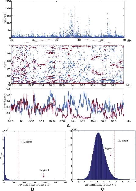
The novel information that is revealed by XP-CLR is best understood by studying examples in which the test finds signals not identified by previous approaches. Figure 7 highlights a 1-Mb region around 38.2 Mb on chromosome 11 that contains an extremely strong XP-CLR signal in the comparison of CEU-YRI populations, but in which both the XP-EHH and iHS scores are not outliers compared with the genome-wide empirical distributions. We manually explored the data pattern in that region to understand the discrepancy. The derived allele frequency distribution in YRI is not unusual, but in CEU, 349 out of 918 SNPs are fixed, and there is a severe reduction of heterozygosity, suggesting a sweep. The sweep is likely to be ancient, since we observed breakdown of LD across hotspots in the region in CEU, explaining why the LD-based XP-EHH tests and iHS tests are not particularly striking. There are no known genes in this region, although there are cDNAs expressed in testes (Wiemann et al. 2001).
Figure 7.
(A, top) The plot of XP-CLR scores along chromosome 11 from the CEU-YRI comparison. (Middle) The derived allele frequencies of SNPs in YRI (blue dots) and CEU (red dots) populations in the zoomed region. (Bottom) Heterozygosity in the same region. (blue line) The average heterozygosity of 20 SNPs in the YRI population; (red line) CEU. (B,C) Histograms of genome-wide XP-CLR scores (B) and XP-EHH scores (C) in the comparison of CEU-YRI populations. The red arrows indicate the ranks of XP-CLR and XP-EHH scores relative to the genome-wide average.
A second example of a novel locus that emerges from the XP-CLR test is a 300-kb region on chromosome 14, containing two major haplotypes that appear to be increased in frequency in CEU relative to YRI (Supplemental Fig. S7). We hypothesize that this reflects selection on standing genetic variation, in which the two haplotypes increased to high frequency in the European population because they were both in LD with the advantageous allele when selection began. The fact that these two haplotypes are very divergent explains why XP-EHH is not significant at the 1% level (XP-EHH searches for a single haplotype that is increased in frequency). This region contains the NRXN3 neurexin protein, which is related to cell adhesion during synaptogenesis. Supplemental Figure S8 shows another locus that potentially reflects selection on standing variation and that is also a novel finding of XP-CLR relative to previous methods that analyzed the same data.
High XP-CLR scores in pigmentation genes and other functional categories
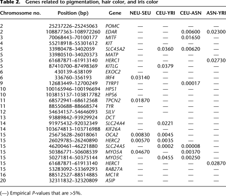
Genes related to pigmentation and hair color have been shown to be enriched in signals of selection, including SLC24A5, SLC45A2, KITLG, OCA2, TYRP1, MLPH, and RGS19 (Sabeti et al. 2007; Pickrell et al. 2009). Our method also found many signals at pigmentation genes and obtained a novel finding at HERC2, which is known to modulate iris color and blonde hair (Han et al. 2008; Kayser et al. 2008) (Supplemental Fig. S9).
To develop a formal test for whether particular sets of genes defined according to their functional category (like pigmentation) are enriched in high XP-CLR scores, we first assigned empirical rank-order-based P-value to each of the genes, taking into account the gene length by permutation. With the XP-CLR scores from a genome-wide scan, we randomly placed the genes in the genome, and recorded the highest XP-CLR score within a distance of 100 kb from the gene. The proportion of XP-CLR scores from the permutations that exceeded the observed score was used as the empirical P-value. We then used a hypergeometric distribution to assess whether the number of genes beyond the 1% cutoff was statistically significant. Table 2 lists the P-values for those pigmentation candidate genes. There is a highly significant enrichment of pigmentation genes under selection in comparisons involving Europeans (P = 1.20 × 10⁻⁸ for CEU-ASN, 1.9 × 10⁻⁴ for CEU-YRI).
Table 2.
Genes related to pigmentation, hair color, and iris color
(—) Empirical P-values that are >5%.
We applied this test to functional categories of genes listed in the Gene Ontology (GO) database (Ashburner et al. 2000). The inflammatory response pathway is significantly enriched in selected loci even after correcting for multiple hypothesis testing using a Benjamini-Hochberg correction (Benjamini and Hochberg 1995) (P = 5.7 × 10⁻⁶ in the CEU-ASN population comparisons). The pathways related to regulation of apoptosis, blood vessels development, protein kinase activity, metabolic process, and immune system activity are also significantly enriched in selected loci (Supplemental Table S3). Interestingly, when we applied this category-based test to sets of genes that have emerged as associated to complex traits from GWA studies, we found no evidence of enrichment for selection at genes associated with Crohn's disease, height, and BMI. However, like Pickrell et al. (2009), we found significant enrichment for selection signals associated with Type-2 diabetes (Supplemental Table S4).
Discussion
We have presented a novel method for detecting natural selection based on multilocus allele frequency differentiation between two populations. Single locus Fst values are highly variable (Weir et al. 2005). To circumvent this problem, recent studies either reported the highest Fst score (Pickrell et al. 2009) or used the average of Fst within a window (Weir et al. 2005). Using a sliding window can reduce variance in Fst measurements, but does not take advantage of the detailed pattern of allele frequency differentiation expected in a selected region. Our method can be viewed as a model-based extension of Fst to multiple-loci. We explicitly model the “spatial” pattern of allele frequencies along a chromosome as a function of the genetic distance to the advantageous allele. Our method is independent of window sizes, as when the studied SNP is far away, the distributions under neutrality and selection converge. By combining information from contiguous SNPs, we increase our power to detect selection. In addition to being a test of neutrality, the method also provides a confidence interval for the position of an advantageous allele with surprisingly good resolution.
We compared the power of XP-CLR in detail to several methods that take advantage of skews in the allele frequency spectrum in a single population to detect signals of selection: the CLR test (Nielsen et al. 2005) and Tajima's D test (Tajima 1989), and showed that our method is more powerful than these two methods for a range of selection scenarios, highlighting the value of taking into account allele frequency differences in surveys for signals of natural selection. We note that Nielsen et al. (2009) recently extended their CLR method into a two-dimensional allele frequency spectrum method, “G2D.” G2D is similar to our method in that both use allele frequency information from two populations. However, the two methods are qualitatively different, and our method achieves functionality that is not achieved by G2D in several respects. First, our method is robust to ascertainment bias, which makes it appropriate for applying to the large SNP array data sets that are already available in diverse human populations, whereas G2D is sensitive to ascertainment bias. Second, our method is robust to uncertainty about the demographic history of a population, in contrast to G2D, which is sensitive to the detailed model of demography that is used. Third, our method takes advantage of the specific “spatial” pattern in the allele frequency skew that is expected to arise around a selected variant, a signal that is not exploited by G2D.
Our method also has some advantages compared with XP-EHH, which has been widely used in searching for signals of selection. Compared with this approach, our method is able to detect older signals (since a strong XP-EHH signal is expected to disappear within several hundred generations due to LD breakdown), and also selection on standing variation. Moreover, phase information is not required by our method and, hence, we can apply it to genotype data without preprocessing steps like phasing that could bias results.
A potential pitfall for our analysis is that we used recombination rates estimated by studying local LD under the assumption of neutrality (Myers et al. 2005), which is expected to provide an underestimate of the true recombination at loci truly affected by selective sweeps (O'Reilly et al. 2008). Encouragingly, however, artifactual estimation of a too-low recombination rate due to selective sweeps is expected to be conservative for our analysis, as it will cause us to underestimate the effect of selection in a region. Moreover, the XP-CLR score is robust to recombination rate uncertainty (Fig. 5).
We conclude that XP-CLR uses a different approach to scan for selection than previous analyses, and thus is able to identify a list of novel regions as potential targets of natural selection. By combining multiple methods—for example, the XP-CLR test, the XP-EHH test, the iHS test, and the CLR test—it should be possible to obtain a richer catalog of likely selective sweeps and a better understanding of how selection has affected human variation.
Methods
Simulation
To generate the null distribution of XP-CLR scores under neutrality, we used coalescent simulations (Hudson 2002). (The software for estimating XP-CLR is publicly available at http://genepath.med.harvard.edu/∼reich.) We chose a number of SNPs to evaluate, and then dropped SNPs randomly if they exceeded this number. We explored a range of demographic histories to address the effect of population history on the null distribution. A recombination rate hotspot model was simulated using msHOT (Hellenthal and Stephens 2007). Selection simulations were carried out via the structured-coalescent scheme with our own code p2S (available on request from HC). To check that the simulation ran correctly, we simulated data under selection for a range of selection intensity levels, and compared observed with predicted Tajima's D. We compared our simulated results with the theoretical prediction for the probability of a lineage escaping from a sweep for a range of r/s values.
Genetic map
We downloaded the genetic map of Myers et al. (2005) from the HapMap webpage (http://www.hapmap.org) and interpolated the genetic positions for each SNP in our data set.
Estimation of test statistics
The list of iHS scores based on HapMap II populations, and the XP-EHH scores for the CEU-YRI comparison, were provided by Pardis Sabeti and Ilya Schlyakhter (Harvard University). The XP-EHH and iHS scores for other populations were calculated with code downloaded from the Pritchard lab web page (http://hgdp.uchicago.edu). The CLR scores were estimated using code provided by Rasmus Nielsen (University of California, Berkeley) and Melissa Hubisz (University of Chicago). We set grid points for CLR tests with an equal spacing of 2 kb along the genome. All site frequency spectra were treated as unfolded. The phased data for HapMap II populations were downloaded from the HapMap FTP server. The software fastPhase (Scheet and Stephens 2006) was used to infer phase for the POPRES samples.
HapMap phase-II data
Except for the Northern–Southern European comparison, all analyses were carried out on 3,619,100 SNPs that had successfully been genotyped in all four HapMap populations. We evaluated grid points for putative advantageous alleles every 2 kb along the genome, and evaluated a window size of 0.2 cM around each grid point. To account for heterogeneity of SNP density across different genomic regions, we fixed the number of SNPs in each window (100). For those windows with more than 100 SNPs, we randomly dropped SNPs until they matched this number. The derived alleles were determined by the comparison with chimpanzee.
Analysis of European data
The Northern and Southern European population samples were obtained from the POPRES data set (Nelsen et al. 2008), restricting to 347,315 SNPs that overlapped with HapMap. The Northern European sample (n = 480) consisted of individuals with ancestry from Denmark, Germany, Norway, Sweden, and the United Kingdom; and the Southern European sample (n = 595) consisted of individuals with ancestry from Greece, Italy, Portugal, Spain, and Tuscany. The window size was chosen to be 0.2 cM and the number of SNPs in each window was fixed equal to be 50. All analyses use Southern Europeans as the reference population. We also carried out an analysis using Northern Europeans as the reference, but the results are not reported here.
Acknowledgments
D.R. was supported by a Burroughs Wellcome Career Development Award in the Biomedical Sciences, and all authors were supported by NIH grants U01 HG004168 and R21 AI064519. We thank Alon Keinan, Alkes Price, and Pardis Sabeti for helpful discussions, and the anonymous reviewers for their valuable critiques. We thank Joseph Pickrell, Melisa Hubisz, and Steve Schaffner for assistance in running their software.
Footnotes
[Supplemental material is available online at http://www.genome.org.]
Article published online before print. Article and publication date are at http://www.genome.org/cgi/doi/10.1101/gr.100545.109.
References
- Akey JM. Constructing genomic maps of positive selection in humans: Where do we go from here? Genome Res. 2009;19:711–722. doi: 10.1101/gr.086652.108. [DOI] [PMC free article] [PubMed] [Google Scholar]
- Akey JM, Zhang G, Zhang K, Jin L, Shriver MD. Interrogating a high-density SNP map for signatures of natural selection. Genome Res. 2002;12:1805–1814. doi: 10.1101/gr.631202. [DOI] [PMC free article] [PubMed] [Google Scholar]
- Ashburner M, Ball CA, Blake JA, Botstein D, Butler H, Cherry JM, Davis AP, Dolinski K, Dwight SS, Eppig JT, et al. Gene Ontology: Tool for the unification of biology. The Gene Ontology Consortium. Nat Genet. 2000;25:25–29. doi: 10.1038/75556. [DOI] [PMC free article] [PubMed] [Google Scholar]
- Benjamini Y, Hochberg Y. Controlling the false discovery rate: A practical and powerful approach to multiple testing. J R Stat Soc Ser B Methodol. 1995;57:289–300. [Google Scholar]
- Carlson CS, Thomas DJ, Eberle MA, Swanson JE, Livingston RJ, Rieder MJ, Nickerson DA. Genomic regions exhibiting positive selection identified from dense genotype data. Genome Res. 2005;15:1553–1565. doi: 10.1101/gr.4326505. [DOI] [PMC free article] [PubMed] [Google Scholar]
- Clark AG, Hubisz MJ, Bustamante CD, Williamson SH, Nielsen R. Ascertainment bias in studies of human genome-wide polymorphism. Genome Res. 2005;15:1496–1502. doi: 10.1101/gr.4107905. [DOI] [PMC free article] [PubMed] [Google Scholar]
- Durrett R, Schweinsberg J. Approximating selective sweeps. Theor Popul Biol. 2004;66:129–138. doi: 10.1016/j.tpb.2004.04.002. [DOI] [PubMed] [Google Scholar]
- Fay JC, Wu CI. Hitchhiking under positive darwinian selection. Genetics. 2000;155:1405–1413. doi: 10.1093/genetics/155.3.1405. [DOI] [PMC free article] [PubMed] [Google Scholar]
- Frazer KA, Ballinger DG, Cox DR, Hinds DA, Stuve LL, Gibbs RA, Belmont JW, Boudreau A, Hardenbol P, Leal SM, et al. A second generation human haplotype map of over 3.1 million SNPs. Nature. 2007;449:851–861. doi: 10.1038/nature06258. [DOI] [PMC free article] [PubMed] [Google Scholar]
- Fu YX, Li WH. Statistical tests of neutrality of mutations. Genetics. 1993;133:693–709. doi: 10.1093/genetics/133.3.693. [DOI] [PMC free article] [PubMed] [Google Scholar]
- Han J, Kraft P, Nan H, Guo Q, Chen C, Qureshi A, Hankinson SE, Hu FB, Duffy DL, Zhao ZZ, et al. A genome-wide association study identifies novel alleles associated with hair color and skin pigmentation. PLoS Genet. 2008;4:e1000074. doi: 10.1371/journal.pgen.1000074. [DOI] [PMC free article] [PubMed] [Google Scholar]
- Hellenthal G, Stephens M. msHOT: Modifying Hudson's ms simulator to incorporate crossover and gene conversion hotspots. Bioinformatics. 2007;23:520–521. doi: 10.1093/bioinformatics/btl622. [DOI] [PubMed] [Google Scholar]
- Hudson RR. Generating samples under a Wright-Fisher neutral model of genetic variation. Bioinformatics. 2002;18:337–338. doi: 10.1093/bioinformatics/18.2.337. [DOI] [PubMed] [Google Scholar]
- Kayser M, Liu F, Janssens AC, Rivadeneira F, Lao O, van Duijn K, Vermeulen M, Arp P, Jhamai MM, van Ijcken WF, et al. Three genome-wide association studies and a linkage analysis identify HERC2 as a human iris color gene. Am J Hum Genet. 2008;82:411–423. doi: 10.1016/j.ajhg.2007.10.003. [DOI] [PMC free article] [PubMed] [Google Scholar]
- Lewontin RC, Krakauer J. Distribution of gene frequency as a test of the theory of the selective neutrality of polymorphisms. Genetics. 1973;74:175–195. doi: 10.1093/genetics/74.1.175. [DOI] [PMC free article] [PubMed] [Google Scholar]
- Lindsay BG. Composite likelihood methods. Contemporary Mathematics. 1988;80:221–239. [Google Scholar]
- Maynard Smith J, Haigh J. The hitch-hiking effect of a favourable gene. Genet Res Camb. 1974;23:23–25. [PubMed] [Google Scholar]
- Myers S, Bottolo L, Freeman C, McVean G, Donnelly P. A fine-scale map of recombination rates and hotspots across the human genome. Science. 2005;310:321–324. doi: 10.1126/science.1117196. [DOI] [PubMed] [Google Scholar]
- Nelsen MR, Bryc K, King KS, Indap A, Boyko AR, Novembre J, Briley LP, Maruyama Y, Waterworth DM, Waeber G, et al. The population reference sample, POPRES: A resource for population, disease, and pharmacological genetic research. Am J Hum Genet. 2008;83:347–358. doi: 10.1016/j.ajhg.2008.08.005. [DOI] [PMC free article] [PubMed] [Google Scholar]
- Nicholson G, Smith AV, Jonsson F, Gustafsson O, Steffanson K, Donnelly P. Assessing population differentiation and isolation from single-nucleotide polymorphism data. J R Stat Soc Ser B Methodol. 2002;64:695–715. [Google Scholar]
- Nielsen R, Hubisz MJ, Clark AG. Reconstituting the frequency spectrum of ascertained single-nucleotide polymorphism data. Genetics. 2004;168:2373–2382. doi: 10.1534/genetics.104.031039. [DOI] [PMC free article] [PubMed] [Google Scholar]
- Nielsen R, Williamson S, Kim Y, Hubisz MJ, Clark AG, Bustamante CD. Genomic scans for selective sweeps using SNP data. Genome Res. 2005;15:1566–1575. doi: 10.1101/gr.4252305. [DOI] [PMC free article] [PubMed] [Google Scholar]
- Nielsen R, Hubisz MJ, Hellmann I, Torgerson D, Andres AM, Albrechtsen A, Gutenkunst R, Adams MD, Cargill M, Boyko A, et al. Darwinian and demographic forces affecting human protein coding genes. Genome Res. 2009;19:838–849. doi: 10.1101/gr.088336.108. [DOI] [PMC free article] [PubMed] [Google Scholar]
- Oleksyk TK, Zhao K, Vega FMDL, Gilbert DA, O'Brien SJ, Smith MW. Identifying selected regions from heterozygosity and divergence using a light-coverage genomic dataset from two human populations. PLoS ONE. 2008;3:e1712. doi: 10.1371/journal.pone.0001712. [DOI] [PMC free article] [PubMed] [Google Scholar]
- O'Reilly PF, Birney E, Balding DJ. Confounding between recombination and selection, and the Ped/Pop method for detecting selection. Genome Res. 2008;18:1304–1313. doi: 10.1101/gr.067181.107. [DOI] [PMC free article] [PubMed] [Google Scholar]
- Pickrell JK, Coop G, Kudaravalli S, Novembre J, Li JZ, Absher D, Srinivasan BS, Barsh GS, Myers RM, Feldman MW, et al. Signals of recent positive selection in a worldwide sample of human populations. Genome Res. 2009;19:826–837. doi: 10.1101/gr.087577.108. [DOI] [PMC free article] [PubMed] [Google Scholar]
- Price AL, Butler J, Patterson N, Capelli C, Pascali VL, Scarnicci F, Ruiz-Linares A, Groop L, Saetta AA, Korkolopoulou P, et al. Discerning the ancestry of European Americans in genetic association studies. PLoS Genet. 2008;4:e236. doi: 10.1371/journal.pgen.0030236. [DOI] [PMC free article] [PubMed] [Google Scholar]
- Sabeti PC, Reich DE, Higgins JM, Levine HZP, Richter DJ, Schaffner SF, Gabriel SB, Platko JV, Patterson NJ, McDonald GJ, et al. Detecting recent positive selection in the human genome from haplotype structure. Nature. 2002;419:832–837. doi: 10.1038/nature01140. [DOI] [PubMed] [Google Scholar]
- Sabeti PC, Varilly P, Fry B, Lohmueller J, Hostetter E, Cotsapas C, Xie X, Byrne EH, McCarroll SA, Gaudet R, et al. Genome-wide detection and characterization of positive selection in human populations. Nature. 2007;449:913–918. doi: 10.1038/nature06250. [DOI] [PMC free article] [PubMed] [Google Scholar]
- Scheet P, Stephens M. A fast and flexible statistical model for large-scale population genotype data: Application to inferring missing genotype and haplotypic phase. Am J Hum Genet. 2006;78:629–644. doi: 10.1086/502802. [DOI] [PMC free article] [PubMed] [Google Scholar]
- Tajima F. Statistical methods for testing the neutral mutations hypothesis by DNA polymorphism. Genetics. 1989;123:585–595. doi: 10.1093/genetics/123.3.585. [DOI] [PMC free article] [PubMed] [Google Scholar]
- Tang K, Thornton KR, Stoneking M. A new approach for using genome scans to detect recent positive selection in the human genome. PLoS Biol. 2007;5:e171. doi: 10.1371/journal.0050171. [DOI] [PMC free article] [PubMed] [Google Scholar]
- Voight BF, Kudaravalli S, Wen X, Pritchard JK. A map of recent positive selection in the human genome. PLoS Biol. 2006;4:446–458. doi: 10.1371/journal.pbio.0040072. [DOI] [PMC free article] [PubMed] [Google Scholar]
- Weir BS, Cardon LR, Anderson AD, Nielsen DM, Hill WG. Measures of human population structure show heterogeneity among genomic regions. Genome Res. 2005;15:1468–1476. doi: 10.1101/gr.4398405. [DOI] [PMC free article] [PubMed] [Google Scholar]
- Wiemann S, Weil B, Wellenreuther R, Gassenhuber J, Glassl S, Ansorge W, Böcher M, Blöcker H, Bauersachs S, Blum H, et al. Toward a catalog of human genes and proteins: Sequencing and analysis of 500 novel complete protein coding human cDNAs. Genome Res. 2001;11:422–435. doi: 10.1101/gr.154701. [DOI] [PMC free article] [PubMed] [Google Scholar]
- Williamson SH, Hubisz MJ, Clark AG, Payseur BA, Bustamante CD, Nielsen R. Localizing recent adaptive evolution in the human genome. PLoS Genet. 2007;3 doi: 10.1371/journal.pgen.0030090. [DOI] [PMC free article] [PubMed] [Google Scholar]


