Abstract
Many epidemiological models for plant disease include host demography to describe changes in the availability of susceptible tissue for infection. We compare the effects of using two commonly used formulations for host growth, one linear and the other nonlinear, upon the outcomes for invasion, persistence and control of pathogens in a widely used, generic model for botanical epidemics. The criterion for invasion, reflected in the basic reproductive number, R0, is unaffected by host demography: R0 is simply a function of epidemiological parameters alone. When, however, host growth is intrinsically nonlinear, unexpected results arise for persistence and the control of disease. The endemic level of infection (I∞) also depends upon R0. We show, however, that the sensitivity of I∞ to changes in R0 > 1 depends upon which underlying epidemiological parameter is changed. Increasing R0 by shortening the infectious period results in a monotonic increase in I∞. If, however, an increase in R0 is driven by increases in transmission rates or by decreases in the decay of free-living inoculum, I∞ first increases (R0 < 2), but then decreases (R0 > 2). This counterintuitive result means that increasing the intensity of control can result in more endemic infection.
Keywords: epidemiological model, R0, endemic equilibrium, disease control strategies, monomolecular growth, logistic growth
1. Introduction
Successful invasion and persistence of a pathogen within a host population depends upon an adequate supply of susceptible hosts. Too little replenishment of susceptible hosts leads to the elimination of the pathogen and, often too, a failure to invade (Anderson & May 1991). For many diseases of plants and animals, infected individuals die or, if they recover, they are immune to reinfection, so that persistence depends upon birth of susceptibles. Host demography is especially important when the generation time of the host is short enough compared with that of the pathogen to impact on the outcome of epidemics. Such dynamics are common for many plant diseases in which the leaf, root or other organs, rather than the individual host plant, comprise the natural population unit among which a pathogen spreads (Gilligan 2002), and where the densities of these organs change during the course of an epidemic as plants grow. Similar host-driven dynamics apply to many viral diseases of invertebrates and short-lived vertebrate hosts (Bowers & Begon 1991; Bowers et al. 1993; Begon & Bowers 1994; Dwyer 1994; White et al. 1996; Bonsall et al. 1999; Briggs et al. 2000; Liu et al. 2007) and to certain diseases of animals (Anderson & May 1981) and humans, most notably HIV/AIDS (Hyman & Stanley 1988; Jacquez et al. 1988; May et al. 1988; Castillo-Chavez et al. 1989). Here, we focus on soil-borne plant diseases, caused by a range of fungal, viral and bacterial pathogens in crops and natural environments, as exemplars of pathogens for which host demography impacts upon epidemic outcomes. Examples of soil-borne plant pathogens include Gaeumannomyces graminis, Rhizoctonia solani and Fusarium solani, in which a single lesion can colonize or kill an entire root.
The inclusion of host demography is biologically appealing because it promotes biological realism in modelling the spread of pathogens through dynamically changing host populations. It is also attractive to epidemiologists and modellers as a simple plausible mechanism to counteract the exhaustion of susceptible hosts, so allowing coexistence of pathogens and hosts consistent with empirical studies of disease in plant and animal populations. The dynamics of these host–pathogen systems are routinely modelled by compartmental susceptible–infected–removed (SIR) epidemic models that incorporate vital dynamics (birth and death of the host population) and from which it is possible to derive criteria for invasion of the pathogen and persistence of both the pathogen and the host (Anderson & May 1991). Host demography has appeared in epidemiological models in several forms, and there have been extensive and mathematically elegant analyses of particular models involving vital dynamics (Busenberg & Hadeler 1990; Busenberg & van den Driessche 1990; Greenhalgh 1990, 1992a,b; Pugliese 1990; Gao & Hethcote 1992; Hethcote & van den Driessche 1995). However, few studies have specifically addressed the isolated effect of growth functions in epidemiological models by explicitly comparing the results of models that differ only in their representation of host demography, although there have been studies of this kind in models where recovery from infection is possible (Mena-Lorcat & Hethcote 1992; Zhou & Hethcote 1994). Very little attention has been given to a systematic analysis of the ways in which the particular functions for host demography can influence epidemiological dynamics of plant pathogens (Gubbins et al. 2000). In this paper, we analyse the dynamics of a simple SIR-type model with vital dynamics involving two commonly used functions for host growth, the monomolecular and logistic functions. We show that the choice of growth function can have unexpected qualitative effects upon the dynamics of the system, and lead to counterintuitive results when using the model to identify effective control strategies for epidemics. The use of the compartmental modelling approach adopted here originates from work on human disease (Kermack & McKendrick 1927; Anderson & May 1991) and is readily generalized to human, livestock and wild-animal as well as botanical epidemics.
Although early investigations of the epidemics caused by plant pathogens seldom included the demographics of the host population (van der Plank 1963; Gilligan 1985, 1990; Brassett & Gilligan 1988), replenishment of susceptible hosts is common in contemporary models (Gilligan 2002, 2008; Jeger et al. 2004; Madden 2006; Madden et al. 2007). The simplest, and often the default, approach to modelling host growth is to introduce an exponential function for the net birth of susceptible hosts into an SIR epidemic model (Madden et al. 2007). A similar approach is widely used to model epidemics in animal populations (Anderson & May 1991). Unlimited growth of the host population is prevented by the density dependent effect of the pathogen in killing hosts. Biological plausibility collapses, however, in the absence of the pathogen, as then the host population grows without bound. Frequently, and especially when considering infection of individual leaves or roots (Gilligan 1985, 2002), but also for invertebrate and some vertebrate and human populations (Anderson & May 1981; Hyman & Stanley 1988; Jacquez et al. 1988; May et al. 1988; Castillo-Chavez et al. 1989; Begon et al. 1992; Bowers et al. 1993; Begon & Bowers 1994), bounded growth functions are introduced to provide more realistic approximations of host–pathogen dynamics. Of particular interest in the case of viral pathogens of forest-insect pests has been whether or not cyclic dynamics are promoted by adding density dependence in host growth (Bowers et al. 1993; Dwyer 1994; White et al. 1996; Bonsall et al. 1999; Liu et al. 2007). In plant epidemiology, the focus has been on improving the realism of the approximation to host demography, by adding bounds to reflect the limited carrying capacity of the field (Gilligan 2002, 2008) and representing phenomena including disease-induced host responses (Gilligan et al. 1997; Bailey & Gilligan 2004; Bailey et al. 2006). We consider epidemics of plant pathogens to be a practical platform and the context for our theoretical work, as in addition to exemplifying systems for which host demography can markedly affect the outcome of epidemics, previous compartmental models of plant disease have been extensively and successfully confronted with data from both experimentally controlled systems and field trials (Gubbins & Gilligan 1996, 1997a,b,c; Gilligan et al. 1997; Bailey & Gilligan 1999, 2004; Bailey et al. 2004, 2005, 2006, 2009).
Two commonly used classes of functions in the context of host dynamics are typified by the monomolecular function (Jeger 1987; Gilligan 1990; Gilligan & Kleczkowski 1997; Madden et al. 2000; Stacey et al. 2004; van den Bosch et al. 2007) and the logistic function (Gilligan & Kleczkowski 1997; Gubbins & Gilligan 1997a; Truscott et al. 1997; Webb et al. 1999, 2000; Park et al. 2001; Gilligan 2002; Bailey & Gilligan 2004; Bailey et al. 2005, 2006; Parnell et al. 2005; Hall et al. 2007). The monomolecular function introduces a simple upper bound on host growth (Gilligan 1990), while the logistic function introduces a nonlinear feedback in the net birth rate of the host population. Accordingly, we use these two functions to analyse the effects of host growth upon the interpretation of epidemiological models for invasion, persistence and control of disease. Specifically, we show that, although the parameters for host growth do not appear in the criteria for pathogen invasion, host demography does affect other pathogen dynamics, notably persistence and the approach to endemic levels. We also show that the responsiveness of the pathogen to control varies with host demography, even when control is effected through changes in the epidemiological parameters. Finally, we show that progressive increases in the intensity of disease control can lead to the counterintuitive result of an increase in endemic levels of disease.
2. Theory and approaches
2.1. Preamble
We motivate the analysis using a model for epidemics of plant disease, taking a particular SIRX formulation within the general compartmental framework outlined by Gilligan (2002, 2008). The model incorporates dual sources of infection, with primary infection arising from ‘free-living’ inoculum (X) and secondary infection occurring by transmission from infected to susceptible hosts, with allowance for different infectious periods for free-living inoculum and infected hosts, typical of many soil-borne plant pathogens. We show below that the invasion characteristics of SIRX epidemics are controlled by simple sums of primary and secondary infection, and note that the principal conclusions from the more generic SIRX model hold for SIR models of plant and animal epidemics with a single (secondary) source of infection.
2.2. The model
The SIRX model is specified by the following set of coupled ordinary differential equations:
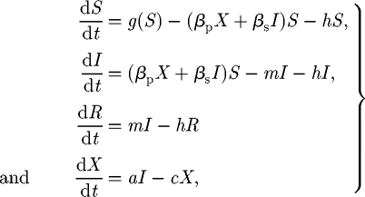 |
2.1 |
with primary infection arising from free-living inoculum (X) and secondary infection occurring by transmission from infected (I) to susceptible (S) hosts, at rates βp and βs, respectively. Rather than necessarily considering a population of individual host plants, host variables may be defined in terms of number or density of plants, roots or leaves, depending upon the natural scale at which symptoms of the epidemic are expressed (Gilligan 1985, 2008). We clarify the approach with a specific example for the ubiquitous take-all pathogen of wheat caused by G. graminis var. tritici, and in which case we would take a single main root axis (adventitious or seminal) as the basic host unit, since the pathogen is capable of incapacitating main root axes and spreads from main root axis to main root axis (Bailey & Gilligan 2004; Bailey et al. 2005, 2006). The numbers of roots of wheat plants increase from 0 to 40 or above over the course of a single season (Bailey et al. 2005), and it is this change we are considering when we refer to demography. Infected hosts remain infectious for m−1 units of time before entering the removed (R) class. New susceptible hosts are produced at rate g(S), with loss of hosts from all classes, for example by natural (non-pathogenic) death or continual harvesting, at rate h. Free-living inoculum decays exponentially at rate c. It is replenished by release from infectious hosts with efficiency a, corresponding to infected hosts either producing or becoming sources of inoculum. This phenomenon is typical of soil-borne plant pathogens (Gubbins & Gilligan 1997a), and has also been modelled in a similar fashion for viral pathogens of insects (Anderson & May 1981; Bowers & Begon 1991; Bowers et al. 1993; Begon & Bowers 1994; Liu et al. 2007). The complex interplay between primary and secondary infection has been previously studied for botanical epidemics (Brassett & Gilligan 1988; Colbach et al. 1997; Gilligan & Kleczkowski 1997; Gubbins & Gilligan 1997a; Truscott et al. 1997; Bailey & Gilligan 1999; Schoeny & Lucas 1999; Gubbins et al. 2000). The dual source of infection is therefore introduced in the epidemiological model but the analyses can easily be simplified to account for secondary infection alone. For convenience, the parameters of the model are summarized in table 1.
Table 1.
Summary of the state variables and parameters.
| symbol | meaning | dimensionless analogue |
|---|---|---|
| S | density of susceptible hosts | Ŝ = S/κ |
| I | density of infected hosts | Î = I/κ |
| R | density of removed hosts | R̂ = bR/mκ |
| X | density of soil-borne inoculum | X̂ = bX/aκ |
| t | time | t̂ = bt |
| g(S) | production of susceptible hosts | n.a. |
| h | rate of removal (all classes of host) | ĥ = h/b |
| f(S) | overall dynamics of susceptible hosts in the absence of infection, where f(S) = g(S) − hS | see below |
| Model M | f(S) = b(κ − S) | f̂(Ŝ) = 1 − Ŝ |
| Model L | f(S) = bS(1 − S/κ) | f̂(Ŝ) = Ŝ(1 − Ŝ) |
| b | birth rate | 1 |
| κ | carrying capacity | 1 |
| βp | rate of primary infection | β̂p = βpaκ/b2 |
| βs | rate of secondary infection | β̂s = βsaκ/b |
| m | rate of disease-induced mortality for infected hosts | 1 |
| a | rate of production of inoculum by infected hosts | 1 |
| c | rate of decay of inoculum | ĉ = c/b |
| μ | total rate at which individuals leave class I, with μ = m + h | μ̂ = μ/b |
2.3. Host demography
Following common practice in compartmental models for plant disease (Gilligan 2002), we compare the effects of two widely used growth functions on epidemiological dynamics. The models differ in the feedback used to limit host growth in the absence of the pathogen. For convenience we merge the production and loss of susceptible hosts into a single function, f(S), with f(S) = g(S) − hS, which controls the dynamics of the host in the absence of the pathogen. We focus upon the monomolecular and logistic models (denoted as models M and L, respectively)
| 2.2 |
| 2.3 |
where in each model b is a rate parameter controlling the rate of production of susceptible hosts, κ is the carrying capacity of the susceptible host population in the absence of the pathogen and q(S) relates the production rate to the current size of the susceptible population. For simplicity, we consider q(S) = S throughout, noting that the qualitative results hold also for forms such as q(S,I) = S + I, in which other classes of host affect the feedback. A derivation of both models is given in appendix A.
2.4. Non-dimensionalization
For convenience we introduce μ = m + h for the combined rates of loss of infected hosts (cf. equation (2.1)). Then introducing the scaled dimensionless variables
| 2.4 |
and the dimensionless parameter groupings
| 2.5 |
transforms the model to
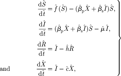 |
2.6 |
with the dimensionless host dynamics in the absence of the pathogen, f̂(Ŝ), given by
| 2.7 |
and
| 2.8 |
Four parameters, the birth rate of susceptible hosts, the carrying capacity, the rate at which inoculum is produced by infected hosts and the rate at which infected hosts transition to the removed class, do not have direct analogues in the dimensionless version of the model after the scaling. Five principal parameters β̂p, β̂s, μ̂, ĉ and ĥ remain, and as these groupings entirely determine the dynamics of the model, we concentrate on these dimensionless analogues of the key epidemiological parameters in our further analysis. The meanings and definitions of the dimensionless parameter groupings are summarized in table 1.
2.5. Methods of analysis
We first determine the reproductive number of the pathogen, R0, to characterize conditions for the pathogen to invade when it is introduced into a population of susceptible hosts at the carrying capacity (Diekmann et al. 1990; Anderson & May 1991; Gubbins et al. 2000). We also perform an explicit stability analysis of the host–pathogen coexistence equilibrium, to confirm that the pathogen and host are able to persist with the other present. Numerical simulation is used to explore the time to equilibrium for both variants (M and L) of the host model. Finally, we analyse the effectiveness of control on endemic levels of infection by characterizing the progressive effect of control through changes in epidemiological parameters.
3. Results
The basic reproductive number of the pathogen is given by (appendix B)
 |
3.1 |
with a natural partitioning (that is useful in later analyses) into independent components corresponding to primary and secondary infection,
| 3.2 |
where Rp0 = β̂p/(μ̂ĉ) and Rs0 = β̂s/(μ̂).
The M model exhibits two equilibria. There is a pathogen-free equilibrium, at which the host is present at its carrying capacity,
| 3.3 |
and a coexistence equilibrium, at which the density of susceptible hosts is depressed below the disease-free value,
 |
3.4 |
There are three equilibria for the L model: a pathogen-free and host-free equilibrium in which both species are eliminated; a pathogen-free equilibrium; and a host–pathogen coexistence equilibrium, given respectively by
| 3.5 |
| 3.6 |
and
 |
3.7 |
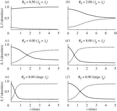
For both models, the equilibrium that is attained in the long term is controlled by the value of R0 (see appendix C for stability analysis). Unsurprisingly, if R0 < 1, the pathogen is unable to invade and is always eradicated, and the models predict that the susceptible host population will stabilize at its carrying capacity. The pathogen-free and host-free equilibrium (equation (3.5)) for model L is unstable and so is unlikely ever to be attained in practice. If R0 > 1, the pathogen is always able to invade and persist in the host population, and both models predict a non-zero density of infected tissue for all time. The models differ, however, with respect to the stability of the coexistence equilibrium. For Model M, the coexistence equilibrium is always stable for R0 > 1, and the density of infected hosts reaches the level predicted by equation (3.4). Even for relatively large values of R0, the equilibrium is attained directly with no oscillatory character to the fixed point (figure 1).
Figure 1.
The behaviour of Model M for different values of R0, showing the susceptible (solid) and infected (dotted) host densities as functions of time. Graphs (a)–(d) illustrate epidemics corresponding to different values of R0. Graphs (d)–(f) illustrate the qualitative similarity between epidemics with the same value of R0 irrespective of the combination of parameters, causing R0 to take a particular value.
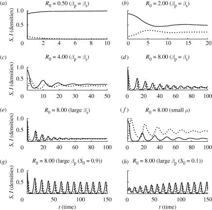
Model L exhibits a more complex behaviour (figure 2). For intermediate values of R0, the behaviour is similar to that of Model M, and the densities of susceptible and infected hosts stabilize at the levels predicted by equation (3.7). For sufficiently large values of R0, however, the coexistence equilibrium of Model L can lose its stability, and a periodic cycle can be generated, with the densities oscillating about their equilibrium values. A large value of Rp0 is required for the oscillations to appear. Moreover, this large value must be attained via increases to the dimensionless analogue of the rate of primary infection β̂p (driven by increases to parameters such as βp or a) rather than by decreases to the dimensionless analogue of the rate of decay of the inoculum ĉ. When it occurs, the amplitude of the limit cycle can be large compared with the equilibrium densities and is entirely independent of the initial conditions (so long as the initial densities of both host and pathogen are non-zero). In general, the size of the oscillations increases with the value of β̂p. We note that even if the parameters are not suitable for the limit cycle to appear, the coexistence equilibrium in Model L is approached by weakly damped oscillations, ensuring that the equilibrium is reached relatively slowly in comparison with Model M.
Figure 2.
The behaviour of Model L for different values of R0, showing the susceptible (solid) and infected (dotted) host densities as functions of time. Comparing graphs (d)–(f) with (g) illustrates the qualitatively different behaviour that is possible for epidemics with the same value of R0, and comparing (g) with (h) illustrates that the amplitude of the limit cycle is independent of the initial condition. Even when the limit cycle is not present, and the coexistence equilibrium is stable (i.e. graphs (b)–(f)), it is attained via damped oscillations and very slowly in comparison with Model M (cf. figure 1). Graph (a) shows the behaviour when the pathogen is unable to invade.
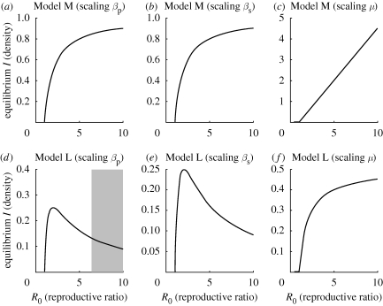
We have shown that the density of infected hosts at equilibrium depends upon R0. More insight is obtained by examining how changes to individual parameters within R0 affect the response (figure 3). The key determinant of the behaviour is whether or not μ̂ (the rate of death/removal of infected hosts) is changing. In particular, for Model M, if the parameter μ̂ is varied in order to alter R0, then the infected density at equilibrium increases indefinitely, whereas if changes to any of the other parameters are driving the change in the reproductive number, the infected density remains bounded (although the density increases with R0 as might be expected). That the infecteds can be unbounded in Model M when there is also a carrying capacity for susceptibles is a subtle point, which can be explained as follows. The behaviour of Model M as R0 increases without bound depends critically upon the parameter that is altered to effect the change. In all cases, a large value of R0 leads to a small number of susceptible hosts at equilibrium, and in Model M the dynamics of host production mean that a relatively large (but bounded) number of new susceptible hosts therefore enter the S compartment per unit time. When any increase to R0 is caused by altering the rate(s) of infection, this bounded rate of influx of new susceptible hosts puts a bound on the maximum number of newly infected hosts per unit time, no matter how large the rates of infection become, and very large increases to the endemic density are effectively constrained by this bounded influx of new hosts rather than by alterations to the rate parameters. This may be contrasted with increasing R0 by decreasing the rate at which infected hosts decay. In this case the non-zero influx of infected hosts ultimately owing to the non-zero birth term cannot be balanced by the ever-decreasing outflow corresponding to disease-induced death, and so there is an unbounded response in endemic density to decreases to μ. That the response with changes to R0 caused by alterations to μ in Model L is not unbounded is due to the low rates of birth at low susceptible density (caused by high R0) specified in the host dynamics of that model.
Figure 3.
The terminal density of infected hosts at the coexistence equilibrium as a function of R0. Graphs (a)–(c) show the behaviour of Model M, whereas graphs (d)–(f) show the behaviour of Model L. The response and stability of the endemic equilibrium depend upon which dimensionless parameter is altered in manipulating the reproductive number. The values of βp for which there is a limit cycle are shaded in (d).
The pattern for the equilibrium density of infected hosts in Model L is more striking. If R0 is increased upwards from the bifurcation at R0 = 1 by decreasing μ̂, there is a monotonic (but bounded) increase in the infected density. If, however, an increase in R0 is driven by appropriate increases in β̂p and β̂s or decreases in ĉ, the density of infected hosts first increases (R0 < 2) but then decreases (R0 > 2). This counterintuitive result has important implications for control (see below). Note that these patterns can be explained analytically by characterizing the response of the equilibrium to the dimensionless parameters: the mathematical details are given in appendix D.
3.1. Control
Control of plant disease is routinely achieved by genetical, chemical, cultural or biological means. Here we interpret the generic effects of control by analysing the effects of changes in the key epidemiological parameters (β̂p, β̂s, μ̂, ĉ) on the dynamics of infection. For example, chemical control may reduce the transmission rates or the infectious periods (Hall et al. 2004), while cultural or biological control may accelerate the decay of inoculum in soil (Cook & Baker 1983). We distinguish between eradication, in which the pathogen is entirely removed from the system and is unable to persist (table 2); and reduction, in which the density of infected hosts is reduced (table 3).
Table 2.
Eradication control (for both variants of the model).
|
R0 of pathogen |
eradication possible with changes to one parameter? |
||||
|---|---|---|---|---|---|
| Rp0 > 1 | Rs0 > 1 | decreasing β̂p | decreasing β̂s | increasing μ̂ | increasing ĉ |
| X | X | √ | √ | √ | √ |
| √ | X | √ | X | √ | √ |
| X | √ | X | √ | √ | X |
| √ | √ | X | X | √ | X |
Table 3.
Reduction control in Model L. (The symbol ↓ indicates that the parameter change in question (which always leads to a decrease in the reproductive number) also leads to a decrease in the density of infected hosts at equilibrium, ↑ indicates that it always leads to an increase and ↑↓ indicates that it leads first to an increase then to a decrease depending upon the magnitude of the change. Note that these results apply only to Model L; the simpler results of analogous changes in Model M are discussed in the main text.)
|
R0 of pathogen |
effect of control on infected host density |
|||||
|---|---|---|---|---|---|---|
| R0 > 2 | Rp0 > 2 | Rs0 > 2 | decreasing β̂p | decreasing β̂s | increasing μ̂ | increasing ĉ |
| X | X | X | ↓ | ↓ | ↓ | ↓ |
| √ | X | X | ↑↓ | ↑↓ | ↓ | ↑↓ |
| √ | √ | X | ↑↓ | ↑ | ↓ | ↑↓ |
| √ | X | √ | ↑ | ↑↓ | ↓ | ↑ |
| √ | √ | √ | ↑ | ↑ | ↓ | ↑ |
The results for eradication are common to both M and L models. Decreasing μ̂ is effective in eradicating the pathogen, irrespective of whether Rp0 > 1, Rs0 > 1, or Rp0, Rs0 > 1 (table 2). The possibility of eradication by altering one of the other parameters depends upon the partitioning of the reproductive number into components for primary and secondary infection. For example, a pathogen with Rs0 > 1 can never be eradicated by changes to the parameters associated with primary infection, even if the rate of primary infection (β̂p) is decreased to zero or if the rate of decay of primary inoculum (ĉ) is increased without bound (table 2). This is simply because R0 ≥ Rs0 > 1. Similarly, if the epidemic is driven by primary infection (and so has Rp0 > 1), then a strategy based around intercropping (which alters the rate of secondary infection β̂s), for example, will never be able to control the disease in an agricultural crop, no matter how much of the available land is turned over to the non-crop species (even in the limit β̂s → 0).
The results for the reduction in endemic levels of pathogen density differ between the two host growth models. Whereas for Model M there is a predictable monotonic response in the endemic level of infection with changes in each of β̂p, β̂s, μ̂ or ĉ, the corresponding responses for Model L are more complex (table 3). It follows that for Model M, the more effort that is put into control, measured by changes in parameter values, the greater the effect in reducing the endemic level of infection (I(t → ∞)). With the exception of changes in μ̂, this is not true for Model L (table 3) because of the non-monotonic response of the endemic level of infection to changes in R0 (figure 3; appendix C). The behaviour depends upon the balance between primary and secondary infection, the magnitude of R0 and the control strategy that is applied. Progressively ramping up the intensity of control to decrease the transmission rates β̂p and β̂s, and so to decrease the value of R0, can lead first to an increase and then to a decrease in the endemic level of infection as the relevant parameter itself and so R0 decreases through 2. A similar result applies to control that progressively increases the loss of inoculum ĉ (table 3).
4. Discussion
We have shown that the selection of commonly used functions for host growth to control the supply of susceptible tissue in epidemiological models can have profound effects on the invasion, persistence and control of plant pathogens. This means that care must be taken not only in coupling host demography with epidemic models to predict disease dynamics, but also in optimizing the effectiveness of control. We have used a combination of non-dimensionalization to simplify an SIRX model, reducing the numbers of free parameters to assist biological interpretation, together with R0 to analyse invasion, and endemic stability analysis to characterize persistence. Following Gubbins et al. (2000), we show that the form of R0 is unaffected by host demography and that for this class of model, R0 is the sum of two distinct components that correspond to primary and secondary infection (Rp0 and Rs0, respectively). This allows us to determine suitable eradication strategies for particular host–pathogen interactions, or alternatively to motivate preventative strategies to stop pathogen invasion. We note that, in particular, a pathogen with Rp0 > 1 can only be eradicated by altering rates associated with primary infection and that there is an analogous result for secondary infection. While this is unsurprising to epidemiologists, it switches the focus to mechanistic and biologically meaningful parameters that affect the dynamics. This differs from conventional assays and analyses of control that have tended to concentrate on physiological responses such as reduction in lesion growth, without translating these effects into epidemiologically meaningful parameters to gauge whether or not control will be successful in arresting epidemiological spread.
Whereas Gubbins et al. (2000) used generic functions for host demography, we have focused on two specific functions, the monomolecular and logistic. Much previous work in botanical epidemiology has included analogous forms, using monomolecular (Jeger 1987; Gilligan 1990; Gilligan & Kleczkowski 1997; Madden et al. 2000; Truscott & Gilligan 2003; Stacey et al. 2004; van den Bosch et al. 2007) or logistic growth (Gilligan & Kleczkowski 1997; Gubbins & Gilligan 1997a; Truscott et al. 1997; Webb et al. 1999, 2000; Park et al. 2001; Gilligan 2002; Bailey & Gilligan 2004; Bailey et al. 2005, 2006; Parnell et al. 2005; Hall et al. 2007). The choice of a particular function was usually arbitrarily determined by selection of a phenomenological description to satisfy the characteristics of host population growth in the absence of infection. The generality of the models in Gubbins et al. (2000) essentially restricted analyses to determining thresholds for invasion only. Here by defining functions explicitly we derive explicit expressions for the density of infected hosts at the endemic equilibrium, and analyse the stability of these equilibria. We find that the extra nonlinearity associated with logistic growth leads to a reduction in endemic stability, and indeed if the parameters are suitable, a limit cycle can appear. We note that, in a previous continuous-time model of viral pathogens of insects with free-living infective stages (Bowers et al. 1993), adding host density dependence has the opposite effect, and reduces the range of parameters for which stable cycles are possible (White et al. 1996). However, their model is a direct elaboration of Anderson & May's (1981) original model, in which both susceptible and infected hosts are able to reproduce. This is not the case in our model, in which infection and the consequent expression of disease prevents an infected unit (which may be a plant, leaf or root, depending upon the pathogen of interest) from contributing fully to the production of new plants, leaves or roots via decreases to the fecundity, the photosynthetic capacity or nutrient uptake of the associated plant, respectively. A more relevant comparison is with models of viral pathogens of insects in which births come from susceptible hosts alone (Dwyer 1994), and for which it is acknowledged that density dependence acts to stabilize cycles (Bonsall et al. 1999). There is also a more recent model of Liu et al. (2007) that investigates the influence of the particular type of density dependence upon the dynamics of these systems and which again concludes that density dependence often promotes cycling. A similar conclusion is apparent from an (arguably) more realistic model of temperate forest insects which includes a discrete-time, between-season component (Bonsall et al. 1999), in which density dependence acts to counteract the strongly destabilizing effects of the time lag (May 1974), and to stabilize the divergent oscillations predicted by the underlying model.
The efficacy of control strategies that reduce but do not eradicate disease were investigated by mapping control onto the non-dimensionalized parameters and examining changes in the endemic levels of infection. For Model M, in which there is a simple linear growth function, the responses are straightforward: the parameters are changed by control to reduce the rate(s) of transmission and/or to increase the rate(s) of decay of infectious material, and so to decrease R0, the terminal density of infected hosts is invariably reduced. However, in Model L, in which there is nonlinear growth, this is not always the case. If R0 > 2, then ramping up the intensity of control can lead to a paradoxical increase in disease, despite the smaller value of R0. The unexpected behaviour depends upon which component of R0 is altered to effect the reduction.
In summary, our results highlight the importance of using epidemiological parameters to analyse the effectiveness of treatments for control. They also emphasize that careful thought should be given to the interplay between host demography and epidemiological dynamics. Although there has been some analysis of the effect of vital dynamics on generic classes of model without reference to particular host–pathogen pairs (Mena-Lorcat & Hethcote 1992; Zhou & Hethcote 1994), there has been no investigation of diseases of plants nor of how demography affects disease control. While we acknowledge that our underlying modelling framework was rather simple, by restricting ourselves to a variant of the SIR framework, we have avoided the proliferation of state variables and parameters which would have been associated with more complex models and avoided obscuring the underlying message of this work. We have also ensured maximum transferability across the widest range of host pathogen systems by using the common currency of the field, and have illustrated our results in a class of model that has been experimentally tested for plant disease (Gubbins & Gilligan 1996, 1997a,b,c; Gilligan et al. 1997; Bailey & Gilligan 1999, 2004; Bailey et al. 2004, 2005, 2006, 2009). We note that previous investigations, including our own (Gilligan et al. 1997; Bailey & Gilligan 2004; Bailey et al. 2006), have focused on elaborations such as disease-induced host responses to infection. Our results here suggest that seemingly benign choices can have unexpected and counterintuitive results in even the simplest models. Future work in the context of plant disease will now analyse interactions induced by alternative forms for host growth and disease-induced host responses to infection.
Acknowledgements
We thank the BBSRC for funding in the form of a PhD studentship (N.J.C.) and a professorial fellowship (C.A.G.). We also thank Stephen Parnell for helpful comments upon an early draft of the paper and the two anonymous referees for their close reading and helpful feedback.
Appendix A. Motivating the growth functions
We present a motivation for the monomolecular and logistic functions used in the main text. In each case we consider the dynamics of the host in the absence of infection, which are controlled by (cf. equation (2.1))
| A 1 |
We consider three plausible scenarios:
I: constant birth rate, with g(S) = r;
II: constant per capita birth rate, with g(S) = rS; and
III: linearly decreasing per capita birth rate, with g(S) = rS(1 − pS);
and determine which lead to biologically plausible (i.e. finite) host densities. In scenario I, we can rewrite f(S) = b(κ − S), where b = h and κ = r/h, and so the model predicts a monomolecular increase in the absence of infection, with well-defined carrying capacity κ. Similarly scenario III leads to f(S) = bS(1 − S/κ) where b = r − h and κ = (r − h)/rp, and so a logistic increase is predicted. However, in scenario II, f(S) = (r − h)S, and so the model predicts an exponential increase in the number or density of susceptible hosts in the absence of infection (if r > h). This is unrealistic, and so scenario II is rejected.
Appendix B. Basic reproductive number
We calculate this key threshold using the next-generation method (Diekmann et al. 1990), which is a general procedure to determine R0 in compartmental models with multiple infectious classes (Heffernan et al. 2005). We choose a permutation of the n = 4 state variables such that the first m = 2 are infected, with x = (Î, X̂, Ŝ, R̂)T, and find (in the notation of van den Driessche & Watmough (2002)) that the disease-free equilibrium is x0 = (0, 0, 1, 0)T, that the operator F, which reflects the rate at which new infections arise, is given by
 |
B 1 |
and that the operator V, which reflects the rate at which compartments corresponding to infection are exited, is given by
 |
B 2 |
Therefore, the next-generation matrix is
 |
B 3 |
and, since R0 is the spectral radius of this matrix (which in this case is just the first element),
 |
B 4 |
Appendix C. Local stability analysis
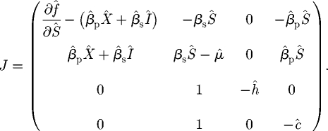
The linear stability of any equilibrium of the model system in equation (2.6) is controlled by the eigenvalues of the Jacobian matrix, which at the general point (Ŝ, Î, R̂, X̂) is given by
 |
C 1 |
It is clear by considering the third column that one eigenvalue is always −ĥ, and so stability is controlled by the ‘deflated’ Jacobian corresponding to the Ŝ, Î and X̂ component:
 |
C 2 |
We use J* to investigate the stability of each equilibrium in turn.
C.1. Pathogen-free and host-free equilibrium (Model L only)
The deflated Jacobian reduces to
 |
C 3 |
from which it is immediately apparent that the additional eigenvalues are 1, −μ̂, −ĉ and so that this equilibrium is always a saddle point (and so is unstable).
C.2. Pathogen-free equilibrium
For both models, the deflated Jacobian becomes
 |
C 4 |
as ∂f̂/∂Ŝ = −1 for both models when Ŝ = 1, and therefore the characteristic equation
| C 5 |
defines the additional eigenvalues λ. Clearly, one eigenvalue is always −1, and the Routh–Hurwitz (R–H) criterion (Britton 2003) applied to the inner quadratic equation indicates that the other eigenvalues will have negative real part if and only if
 |
C 6 |
The rearrangement of this pair of inequalities
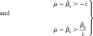 |
C 7 |
indicates that if the second condition is satisfied, then the first is definitely true, and therefore that it is sufficient to work with the second inequality. However, the second inequality may be rearranged as
 |
C 8 |
indicating that R0 < 1 is a necessary and sufficient condition for all three eigenvalues to have negative real part (or equivalently for the pathogen-free equilibrium to be stable). As the R–H criterion is a two-way implication, we also see that whenever R0 > 1 that the pathogen-free equilibrium is definitely unstable, and that the pathogen is always able to initially invade a host population at its carrying capacity.
An equivalent result is derived directly using the next-generation method in appendix B; the preceding analysis is included to motivate the more complex analysis that follows.
C.3. Coexistence equilibrium
Noting that at this equilibrium β̂pX̂ + β̂sÎ = μ̂Î/Ŝ, the deflated Jacobian may be rewritten as
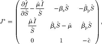 |
C 9 |
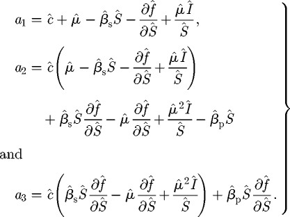
which after some algebra indicates that the characteristic equation is given by
| C 10 |
with coefficients
 |
C 11 |
The R–H criterion for cubic equations indicates that the additional eigenvalues have negative real part, and so the coexistence equilibrium is stable whenever the three conditions
 |
C 12 |
are simultaneously satisfied.
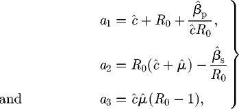
In the case of Model M, it is possible to simplify the formidable looking expressions in equation (C 11) and to prove explicitly that the R–H criterion is satisfied at the coexistence equilibrium. The coefficients of the characteristic equation may be reduced to
 |
C 13 |
from which it is clear that the first two parts of the R–H criterion in equation (C 12) are definitely satisfied whenever R0 > 1. After some rearrangement, we see that
 |
C 14 |
and as the right-hand side contains only positive terms, the sufficiency of the condition R0 > 1 for stability of the pathogen-present equilibrium in Model M is proved.
However, it is impossible to adapt this analysis for Model L. In fact, with logistic host dynamics the condition R0 > 1 does not guarantee that the pathogen-present equilibrium is stable, and for certain sets of parameters it is possible to have R0 > 1, but a1a2 − a3 < 0, and so eigenvalues with real parts of mixed sign. This indicates that the coexistence equilibrium is unstable for these sets of parameters. However, as R0 > 1, the pathogen-free equilibrium is also unstable, and as we know that the trivial equilibrium of Model L is always unstable, none of the three equilibria can be attained in the long term. In fact, as the parameters are changed through the threshold at which a1a2 − a3 = 0, there is a Hopf bifurcation, with the associated loss of stability of the coexistence equilibrium (via a pair of complex eigenvalues bifurcating to have a positive real part (Glendinning 1994)). The system exhibits a periodic limit cycle, with the densities of all three state variables forever oscillating around their respective equilibrium values. It is possible to determine a condition upon the parameters that ensures the existence of the periodic cycle, but it is difficult to interpret. However, extensive numerical work indicates that the cycle requires a large rate of primary infection, β̂p.
Appendix D. Variation of the infected density with changes to the dimensionless parameters
In Model M, the partial derivatives of the endemic infected host density are given by
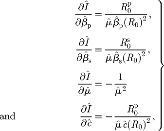 |
D 1 |
and so there is always an increase in the density of infected hosts with any increase in the transmission rates and/or a decrease in the infectious periods. However, in Model L, the corresponding expressions are
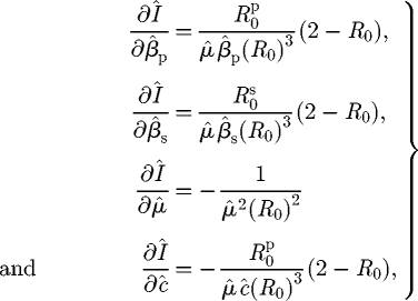 |
D 2 |
and so (for all parameters except μ̂) the behaviour depends upon whether or not R0 is greater than 2, as described in the main text.
References
- Anderson R. M., May R. M. 1981. The population dynamics of microparasites and their invertebrate hosts. Phil. Trans. R. Soc. Lond. B 291, 451–524. ( 10.1098/rstb.1981.0005) [DOI] [PMC free article] [PubMed] [Google Scholar]
- Anderson R. M., May R. M. 1991. Infectious diseases of humans. Oxford, UK: Oxford University Press. [Google Scholar]
- Bailey D. J., Gilligan C. A. 1999. Dynamics of primary and secondary infection in take-all epidemics. Phytopathology 89, 84–91. ( 10.1094/PHYTO.1999.89.1.84) [DOI] [PubMed] [Google Scholar]
- Bailey D. J., Gilligan C. A. 2004. Modeling and analysis of disease-induced host growth in the epidemiology of take-all. Phytopathology 94, 535–540. ( 10.1094/PHYTO.2004.94.5.535) [DOI] [PubMed] [Google Scholar]
- Bailey D. J., Kleczkowski A., Gilligan C. A. 2004. Epidemiological dynamics and the efficiency of biological control of soil-borne disease in consecutive crops. New Phytol. 161, 561–575. ( 10.1111/j.1469-8137.2004.00973.x) [DOI] [PubMed] [Google Scholar]
- Bailey D. J., Paveley N., Pillinger C., Foulkes J., Spink J., Gilligan C. A. 2005. Epidemiology and chemical control of take-all on seminal and adventitious roots of wheat. Phytopathology 95, 62–68. ( 10.1094/PHYTO-95-0062) [DOI] [PubMed] [Google Scholar]
- Bailey D. J., Kleczkowski A., Gilligan C. A. 2006. An epidemiological analysis of the role of disease-induced root growth in the differential response of two cultivars of winter wheat to infection by Gaeumannomyces graminis var. tritici. Phytopathology 96, 510–516. ( 10.1094/PHYTO-96-0510) [DOI] [PubMed] [Google Scholar]
- Bailey D. J., Paveley N., Spink J., Lucas P., Gilligan C. A. 2009. Epidemiological analysis of take-all decline in winter wheat. Phytopathology 99, 861–868. ( 10.1094/PHYTO-99-7-0861) [DOI] [PubMed] [Google Scholar]
- Begon M., Bowers R. G. 1994. Host–host–pathogen models and microbial pest control: the effect of host self regulation. J. Theor. Biol. 169, 275–287. ( 10.1006/jtbi.1994.1148) [DOI] [PubMed] [Google Scholar]
- Begon M., Bowers R. G., Kadianakis N., Hodgkinson D. E. 1992. Disease and community structure: the importance of host self-regulation in a host–host–pathogen model. Am. Nat. 139, 1131–1150. ( 10.1086/285379) [DOI] [Google Scholar]
- Bonsall M. B., Godfray H. C. J., Briggs C. J., Hassell M. P. 1999. Does host self-regulation increase the likelihood of insect–pathogen population cycles? Am. Nat. 153, 228–235. ( 10.1086/303161) [DOI] [PubMed] [Google Scholar]
- Bowers R. G., Begon M. 1991. A host–host–pathogen model with free-living infective stages, applicable to microbial pest control. J. Theor. Biol. 148, 305–329. ( 10.1016/S0022-5193(05)80240-1) [DOI] [PubMed] [Google Scholar]
- Bowers R. G., Begon M., Hodgkinson D. E. 1993. Host–pathogen population cycles in forest insects? Lessons from simple models reconsidered. Oikos 67, 529–538. ( 10.2307/3545365) [DOI] [Google Scholar]
- Brassett P. R., Gilligan C. A. 1988. A model for primary and secondary infection in botanical epidemics. Zeitschrift fuer Pflanzenkrankheiten und Pflanzenschutz 95, 352–360. [Google Scholar]
- Briggs C. J., Sait S. M., Begon M., Thompson D. J., Godfray H. C. J. 2000. What causes generation cycles in populations of stored-product moths? J. Anim. Ecol. 69, 352–366. ( 10.1046/j.1365-2656.2000.00398.x) [DOI] [Google Scholar]
- Britton N. F. 2003. Essential mathematical biology. London, UK: Springer. [Google Scholar]
- Busenberg S., Hadeler K. P. 1990. Demography and epidemics. Math. Biosci. 101, 63–74. ( 10.1016/0025-5564(90)90102-5) [DOI] [PubMed] [Google Scholar]
- Busenberg S., van den Driessche P. 1990. Analysis of a disease transmission model in a population with varying size. J. Math. Biol. 28, 257–270. ( 10.1007/BF00178776) [DOI] [PubMed] [Google Scholar]
- Castillo-Chavez C., Cooke K., Huang W., Levin S. A. 1989. On the role of long incubation periods in the dynamics of acquired immunodeficiency syndrome (AIDS). Part 1: single population models. J. Math. Biol. 27, 373–398. ( 10.1007/BF00290636) [DOI] [PubMed] [Google Scholar]
- Colbach N., Lucas P., Meynard J. M. 1997. Influence of crop management on take-all development and disease cycles on winter wheat. Phytopathology 87, 26–32. ( 10.1094/PHYTO.1997.87.1.26) [DOI] [PubMed] [Google Scholar]
- Cook R. J., Baker K. F. 1983. The nature and practice of biological control of plant pathogens. St Paul, MN: American Phytopathological Society. [Google Scholar]
- Diekmann O., Heesterbeek J. A. P., Metz J. A. J. 1990. On the definition and the computation of the basic reproductive ratio R0 in models for infectious diseases in heterogeneous populations. J. Math. Biol. 28, 365–382. ( 10.1007/BF00178324) [DOI] [PubMed] [Google Scholar]
- Dwyer G. 1994. Density-dependence and spatial structure in the dynamics of insect pathogens. Am. Nat. 143, 533–562. ( 10.1086/285619) [DOI] [Google Scholar]
- Gao L. Q., Hethcote H. W. 1992. Disease transmission models with density-dependent demographics. J. Math. Biol. 30, 717–731. ( 10.1007/BF00173265) [DOI] [PubMed] [Google Scholar]
- Gilligan C. A. 1985. Construction of temporal models: III. Disease progress of soil-borne pathogens. In Mathematical modelling of crop disease (ed. Gilligan C. A.). London, UK: Academic Press. [Google Scholar]
- Gilligan C. A. 1990. Mathematical modeling and analysis of soilborne pathogens. In Epidemics of plant diseases: mathematical analysis and modeling (ed. Kranz J.), pp. 96–142. Heidelberg, Germany: Springer-Verlag. [Google Scholar]
- Gilligan C. A. 2002. An epidemiological framework for disease management. In Advances in botanical research, vol. 38, pp. 1–64. London, UK: Academic Press; ( 10.1016/S0065-2296(02)38027-3) [DOI] [Google Scholar]
- Gilligan C. A. 2008. Sustainable agriculture and plant disease: an epidemiological perspective. Phil. Trans. R. Soc. B 363, 741–759. ( 10.1098/rstb.2007.2181) [DOI] [PMC free article] [PubMed] [Google Scholar]
- Gilligan C. A., Kleczkowski A. 1997. Population dynamics of botanical epidemics involving primary and secondary infection. Proc. R. Soc. Lond. B 352, 591–608. ( 10.1098/rstb.1997.0040) [DOI] [Google Scholar]
- Gilligan C. A., Gubbins S., Simons S. A. 1997. Analysis and fitting of an SIR model with host response to infection load for a plant disease. Phil. Trans. R. Soc. Lond. B 352, 353–364. ( 10.1098/rstb.1997.0026) [DOI] [Google Scholar]
- Glendinning P. 1994. Stability, instability and chaos: an introduction to the theory of nonlinear differential equations. Cambridge, UK: Cambridge University Press. [Google Scholar]
- Greenhalgh D. 1990. An epidemic model with a density-dependent death rate. IMA J. Math. Appl. Med. Biol. 7, 1–26. ( 10.1093/imammb/7.1.1) [DOI] [PubMed] [Google Scholar]
- Greenhalgh D. 1992a. Some results for an SEIR epidemic model with density dependence in the death rate. IMA J. Math. Appl. Med. Biol. 9, 67–106. ( 10.1093/imammb/9.2.67) [DOI] [PubMed] [Google Scholar]
- Greenhalgh D. 1992b. Some threshold and stability results for epidemic models with a density-dependent death rate. Theor. Popul. Biol. 42, 130–151. ( 10.1016/0040-5809(92)90009-I) [DOI] [PubMed] [Google Scholar]
- Gubbins S., Gilligan C. A. 1996. Population dynamics of a parasite and hyperparasite in a closed system: model analysis and parameter estimation. Proc. R. Soc. Lond. B 263, 1071–1078. ( 10.1098/rspb.1996.0158) [DOI] [Google Scholar]
- Gubbins S., Gilligan C. A. 1997a. Biological control in a disturbed environment. Phil. Trans. R. Soc. Lond. B 352, 1935. –1949. ( 10.1098/rstb.1997.0180) [DOI] [Google Scholar]
- Gubbins S., Gilligan C. A. 1997b. Persistence of host–parasite interactions in a disturbed environment. J. Theor. Biol. 188, 241–258. ( 10.1006/jtbi.1997.0466) [DOI] [Google Scholar]
- Gubbins S., Gilligan C. A. 1997c. A test of heterogeneous mixing as a mechanism for ecological persistence in disturbed environments. Proc. R. Soc. Lond. B 264, 227–232. ( 10.1098/rspb.1997.0032) [DOI] [Google Scholar]
- Gubbins S., Gilligan C. A., Kleczkowski A. 2000. Population dynamics of plant–parasite interactions: thresholds for invasion. Theor. Popul. Biol. 57, 219–234. ( 10.1006/tpbi.1999.1441) [DOI] [PubMed] [Google Scholar]
- Hall R. J., Gubbins S., Gilligan C. A. 2004. Invasion of drug and pesticide resistance is determined by a trade-off between biocide efficacy and relative fitness. Bull. Math. Biol. 66, 835–840. ( 10.1016/j.bulm.2003.11.006) [DOI] [PubMed] [Google Scholar]
- Hall R. J., Gubbins S., Gilligan C. A. 2007. Evaluating the performance of chemical control in the presence of resistant pathogens. Bull. Math. Biol. 69, 525–537. ( 10.1007/s11538-006-9139-z) [DOI] [PubMed] [Google Scholar]
- Heffernan J. M., Smith R. J., Wahl L. M. 2005. Perspectives on the basic reproductive ratio. J. R. Soc. Interface 2, 281–293. ( 10.1098/rsif.2005.0042) [DOI] [PMC free article] [PubMed] [Google Scholar]
- Hethcote H. W., van den Driessche P. 1995. An SIS epidemic model with variable population size and a delay. J. Math. Biol. 34, 177–194. ( 10.1007/BF00178772) [DOI] [PubMed] [Google Scholar]
- Hyman J. M., Stanley E. A. 1988. Using mathematical models to understand the AIDS epidemic. Math. Biosci. 90, 415–473. ( 10.1016/0025-5564(88)90078-8) [DOI] [Google Scholar]
- Jacquez J. A., Simon C. P., Koopman J., Sattenspiel L., Perry T. 1988. Modeling and analysing HIV transmission: the effect of contact patterns. Math. Biosci. 92, 119–199. ( 10.1016/0025-5564(88)90031-4) [DOI] [Google Scholar]
- Jeger M. J. 1987. The influence of root growth and inoculum density on the dynamics of root disease epidemics: theoretical analysis. New Phytol. 107, 459–478. ( 10.1111/j.1469-8137.1987.tb00197.x) [DOI] [PubMed] [Google Scholar]
- Jeger M. J., Holt J., van den Bosch F., Madden L. V. 2004. Epidemiology of insect-transmitted plant viruses: modelling disease dynamics and control interventions. Physiol. Entomol. 29, 291–304. ( 10.1111/j.0307-6962.2004.00394.x) [DOI] [Google Scholar]
- Kermack W. O., McKendrick A. G. 1927. A contribution to the mathematical theory of epidemics. Proc. R. Soc. Lond. A 115, 700–721. ( 10.1098/rspa.1927.0118) [DOI] [Google Scholar]
- Liu W.-C., Bonsall M. B., Godfray H. C. J. 2007. The form of host density-dependence and the likelihood of host–pathogen cycles in forest-insect systems. Theor. Popul. Biol. 72, 86–95. ( 10.1016/j.tpb.2007.01.002) [DOI] [PubMed] [Google Scholar]
- Madden L. V. 2006. Botanical epidemiology: some key advances and its continuing role in disease management. Eur. J. Plant Pathol. 115, 3–23. ( 10.1007/s10658-005-1229-5) [DOI] [Google Scholar]
- Madden L. V., Jeger M. J., van den Bosch F. 2000. A theoretical assessment of the effects of vector-virus transmission mechanism on plant virus disease epidemics. Phytopathology 90, 576–594. ( 10.1094/PHYTO.2000.90.6.576) [DOI] [PubMed] [Google Scholar]
- Madden L. V., Hughes G., van den Bosch F. 2007. The study of plant disease epidemics. St Paul, MN: American Phytopathological Society. [Google Scholar]
- May R. M. 1974. Stability and complexity in model ecosystems. Princeton, NJ: Princeton University Press. [Google Scholar]
- May R. M., Anderson R. M., McLean A. R. 1988. Possible demographic consequences of HIV/AIDS epidemics: I. Assuming HIV infection always leads to AIDS. Math. Biosci. 90, 475–505. ( 10.1016/0025-5564(88)90079-X) [DOI] [Google Scholar]
- Mena-Lorcat J., Hethcote H. W. 1992. Dynamic models of infectious diseases as regulators of population sizes. J. Math. Biol. 30, 693–716. ( 10.1007/BF00173264) [DOI] [PubMed] [Google Scholar]
- Park A. W., Gubbins S., Gilligan C. A. 2001. Invasion and persistence of plant parasites in a spatially structured host population. Oikos 94, 162–174. ( 10.1034/j.1600-0706.2001.10489.x) [DOI] [Google Scholar]
- Parnell S., Gilligan C. A., van den Bosch F. 2005. Small-scale fungicide spray heterogeneity and the coexistence of resistant and sensitive pathogen strains. Phytopathology 95, 632–639. ( 10.1094/PHYTO-95-0632) [DOI] [PubMed] [Google Scholar]
- Pugliese A. 1990. Population models for diseases with no recovery. J. Math. Biol. 28, 65–82. ( 10.1007/BF00171519) [DOI] [PubMed] [Google Scholar]
- Schoeny A., Lucas P. 1999. Modeling of take-all epidemics to evaluate the efficacy of a new seed-treatment fungicide on wheat. Phytopathology 89, 954–961. ( 10.1094/PHYTO.1999.89.10.954) [DOI] [PubMed] [Google Scholar]
- Stacey A. J., Truscott J. E., Asher M. J. C., Gilligan C. A. 2004. A model for invasion and spread of rhizomania in the UK: implications for disease control strategies. Phytopathology 94, 209–215. ( 10.1094/PHYTO.2004.94.2.209) [DOI] [PubMed] [Google Scholar]
- Truscott J. E., Gilligan C. A. 2003. Response of a deterministic epidemiological system to a stochastically varying environment. Proc. Natl Acad. Sci. USA 100, 9067–9072. ( 10.1073/pnas.1436273100) [DOI] [PMC free article] [PubMed] [Google Scholar]
- Truscott J. E., Webb C. R., Gilligan C. A. 1997. Asymptotic analysis of an epidemic model with primary and secondary infection. Bull. Math. Biol. 59, 1101–1123. ( 10.1007/BF02460103) [DOI] [PubMed] [Google Scholar]
- van den Bosch F., Jeger M. J., Gilligan C. A. 2007. Disease control and its selection for damaging plant virus strains in vegetatively propagated staple food crops; a theoretical assessment. Proc. R. Soc. B 274, 11–18. ( 10.1098/rspb.2006.3715) [DOI] [PMC free article] [PubMed] [Google Scholar]
- van den Driessche P., Watmough J. 2002. Reproduction numbers and sub-threshold endemic equilibria for compartmental models of disease transmission. Math. Biosci. 180, 29–48. ( 10.1016/S0025-5564(02)00108-6) [DOI] [PubMed] [Google Scholar]
- van der Plank J. E. 1963. Plant diseases: epidemics and control. London, UK: Academic Press. [Google Scholar]
- Webb C. R., Gilligan C. A., Asher M. J. C. 1999. A model for the temporal buildup of Polymyxa betae. Phytopathology 89, 30–38. ( 10.1094/PHYTO.1999.89.1.30) [DOI] [PubMed] [Google Scholar]
- Webb C. R., Gilligan C. A., Asher M. J. C. 2000. Modelling the effect of temperature on the dynamics of Polymyxa betae. Plant Pathol. 49, 600–607. ( 10.1046/j.1365-3059.2000.00483.x) [DOI] [Google Scholar]
- White A., Begon M., Bowers R. G. 1996. Population cycles in self-regulated insect pathogen systems: resolving conflicting predictions. Am. Nat. 148, 220–225. ( 10.1086/285921) [DOI] [Google Scholar]
- Zhou J., Hethcote H. W. 1994. Population size dependent incidence in models for diseases without immunity. J. Math. Biol. 32, 809–834. ( 10.1007/BF00168799) [DOI] [PubMed] [Google Scholar]


