Inferring cluster-based networks from differently stimulated multiple time-course gene expression data

Abstract

Motivation: Clustering and gene network inference often help to predict the biological functions of gene subsets. Recently, researchers have accumulated a large amount of time-course transcriptome data collected under different treatment conditions to understand the physiological states of cells in response to extracellular stimuli and to identify drug-responsive genes. Although a variety of statistical methods for clustering and inferring gene networks from expression profiles have been proposed, most of these are not tailored to simultaneously treat expression data collected under multiple stimulation conditions.

Results: We propose a new statistical method for analyzing temporal profiles under multiple experimental conditions. Our method simultaneously performs clustering of temporal expression profiles and inference of regulatory relationships among gene clusters. We applied this method to MCF7 human breast cancer cells treated with epidermal growth factor and heregulin which induce cellular proliferation and differentiation, respectively. The results showed that the method is useful for extracting biologically relevant information.

Availability: A MATLAB implementation of the method is available from http://csb.gsc.riken.jp/yshira/software/clusterNetwork.zip

Contact: yshira@riken.jp

Supplementary information: Supplementary data are available at Bioinformatics online.

1 INTRODUCTION

1.1 Time-course gene expression data collected under multiple stimulation conditions

In recent years, a large amount of time-course gene expression data has been collected. This data should help to unravel the mechanisms of cellular processes such as differentiation, transformation and development. To extract valuable information from these data, a variety of statistical approaches for clustering and gene network inference have been proposed. Clustering is one of the most important statistical methods for analyzing gene expression data, since genes sharing similar expression patterns tend to have common biological functions or regulatory mechanisms. Regarding time-course microarray data, several model-based clustering methods have been proposed (Luan and Li, 2003; Ramoni et al., 2002; Wu et al., 2005). On the other hand, the direct inference of gene regulatory networks using mathematical models is another important approach for predicting gene functions. Several methods have been proposed for this purpose, such as dynamic Bayesian networks (DBN) (Imoto et al., 2002; Kim et al., 2003; Perrin et al., 2003; Zou and Conzen, 2005), S-systems (Kikuchi et al., 2003; Kimura et al., 2005), Boolean networks (Martin et al., 2007), state-space models (Beal et al., 2005; Hirose et al., 2008; Rangel et al., 2004; Yamaguchi et al., 2007), discriminant approaches (Kimura et al., 2009) and so on.

Most existing methods are designed for treating data under a single condition. However, in many situations, it is important to deal with differently stimulated multiple time-course gene expression data:

1. It is widely known that distinct extracellular stimulations lead to different cell fates (Kao et al., 2001; Nagashima et al., 2007; York et al., 2000). If different growth hormones elicit distinct phenotypes of cancer cells (such as proliferation or apoptosis), specific network regulators, which are responsible for condition-specific biological outcomes, will become potential drug targets (Bromberg et al., 2008; Miller-Jensen et al., 2007). Therefore, understanding the mechanism of distinct cell decisions induced by different stimulations is one of the most important problems of cell biology.

2. Estimation of a regulatory network from single time-course data results in redundant answers because in most cases, more than one network structure can explain the expression pattern of genes. Many biologists believe that a number of gene expression patterns with some perturbations, e.g. adding some kind of inhibitor, will eliminate the redundancy of associable network structures. For protein-signaling network, it is shown that collecting multifariously perturbed data is very helpful for accurate network specification (Sachs et al., 2005).

Although a large amount of time-course gene expression data collected under stimulation conditions is now available, there is little argument on how to treat such data. Therefore, new statistical methods for clustering or gene network inference which can deal with differently stimulated multiple time-course gene expression data are necessary.

1.2 Relationship between clustering and gene network inference

Clustering and gene network inference methods are usually developed independently. However, we would argue that there are deep relationships between the two and that they potentially cover each other's shortcomings.

Clustering techniques are useful for inferring gene networks. The most difficult factor in inferring gene networks is that the number of genes is so large that the regulatory networks are too complex to elucidate from a limited amount of data. To treat a large number of genes, some types of complexity reduction of the network are inevitable. Since genes sharing similar temporal profiles are considered to be regulated by the same mechanism, exploring networks at the level of gene clusters is a reasonable approach. This is statistically advantageous as the effective dimensions of the networks over the clusters are greatly lower than those over the genes. Therefore, one possible framework is to divide genes into sets of clusters via a clustering method and then infer networks over the clusters (e.g. Martin et al., 2007; Toh and Horimoto, 2002). However, the results of clustering are often accompanied by uncertainty since they depend on the type of clustering method, the choice of distance function and the initialization of parameters. Fixing uncertain sets of clusters for exploring the network is somewhat problematic.

On the other hand, considering network structures helps the clustering methods because the probabilistic model used in clustering becomes more realistic for explaining the temporal gene expression profiles. A large proportion of clustering algorithms can be described within the framework of model-based clustering (Fraley and Raftery, 2002; Zhong and Ghosh, 2003), in which some underlying generative models for the data are assumed. Although many model-based clustering algorithms for time-course microarray data have been proposed (Luan and Li, 2003; Ramoni et al., 2002; Wu et al., 2005), they assume independence of clusters and do not model interactions or regulatory relationships among clusters. Since, regulatory relationships among genes obviously exist (Amit et al., 2007), it makes sense to incorporate the regulatory relationships among clusters into a probabilistic model.

On the basis of these observations, we believe that clustering and gene network inference should be implemented in a unified probabilistic framework. This will remove the necessity of choosing the clustering method to be used before performing gene network inference. Furthermore, generative models assumed in this framework capture the real biological systems better.

Segal et al. (2005) and Inoue et al. (2007) have performed related studies. Segal et al. (2005) proposed a Bayesian network model that explicitly partitions the variables into clusters, so that the variables in each cluster share the same parents in the network and the same conditional probability distribution. However, this approach is applicable only for static data. Inoue et al. (2007) proposed a model-based approach to unify clustering and network modeling using state-space models. Since this method is based on the Bayesian approach, uncertainty analyses of estimated networks are possible via obtained posterior distributions. However, the computational task using Markov chain Monte Carlo requires advanced techniques. Furthermore, the method of Inoue et al. (2007) cannot deal with time-course data in multiple biological conditions.

1.3 Proposal

In this article, we propose a new statistical method for cluster-based gene network inference, which can treat multiple, differently stimulated temporal profiles. Our method simultaneously predicts clusters of temporal expression profiles, relationships between clusters and those between clusters and stimuli. In summary, our goal is to infer a network such as that in Figure 1. Note that our method can also be used for single conditioned data.

Fig. 1.

An image for the network of gene clusters and stimulations.

2 METHODS

2.1 Canonical cluster restriction on state-space models

2.1.1 State-space models

Let us begin with a review of state-space models (see, e.g. Harvey, 1989). Let y_t=(y_1,t,…, y_N,t)′ denote an N-dimensional observed vector at the t-th time step where t=1,…, T. In the context of gene network analysis, y_t usually denote the amounts of gene expression and N is the number of concerned genes. A sequence of the observed vectors is assumed to be generated from the K-dimensional hidden state variable denoted by x_t=(x_1,t,…, x_{K, t})′. The basic form of state space models can be described by the following two equations:

(1)

(2)

where C is an N × K matrix, and A is a K × K matrix. w_t ∼ N(0, Q) and v_t ∼ N(0, R) are noises. Equation (1) is often called the ‘observation model’, while Equation (2) is the ‘system model’. A remarkable feature of state-space models is that they reduce the complexity of regulations from O(N²) to O(K²) by considering regulatory relationships not among genes but among state variables. Several studies (Beal et al., 2005; Hirose et al., 2008; Rangel et al., 2004; Yamaguchi et al., 2007) have proposed the use of state-space models with some modifications for inference of gene networks.

One of the problems with state-space models is that they lack identifiability. That is to say, the representation of state-space models is not uniquely determined. A transformation of state variables x_t^*=Hx_t via any non-singular matrix H yields an essentially equivalent form of the original model:

(3)

(4)

where v^*_t ∼ N(0, HQH′). Hence, by considering C^* = CH⁻¹, x_t^*=Hx_t, A^*=HAH⁻¹ and Q^*=HQH′, the state-space model can be transformed into an equivalent form. Some studies (Hirose et al., 2008; Yamaguchi et al., 2007) proposed restricting the parameter spaces of state-space models, so as to avoid the lack of identifiability. Furthermore, since the lack of identifiability leads to redundancy of state variables and its system models, it is difficult to interpret state variables or estimated parameters.

2.1.2 Canonical cluster restriction

To avoid the lack of identifiability, we propose restricting the parameter spaces as follows:

1. Q=τ²I, τ²>0,

2. each row of C is a vector with only one non-zero element whose value is 1 and

3. each column of C is a non-zero vector.

We call this restriction the canonical cluster restriction. This condition is a key ingredient of the probabilistic model for cluster-based networks. Under this condition, the matrix C={c_n,k} represents the cluster to which each gene belongs. If c_n,k=1, the n-th gene is a member of the k-th cluster. The temporal profile of the n-th gene (y_n,1,…, y_n,T) becomes the temporal profile of the state variables (x_k,1,…, x_k,T) plus noise. Therefore, each (x_k,1,…, x_k,T), k=1,…, K then has an explicit meaning as the cluster center for profiles of corresponding genes, and parameter A represents relationships among clusters. Furthermore, the canonical cluster restriction makes state-space models canonical modulo permutations.

Proposition 1. —

Suppose that the matrix H produced the equivalent form of the state-space model under the canonical cluster restriction, then H has to be a permutation matrix.

Proof. —

Since Q is an identity matrix, the matrix H has to be an orthonormal matrix multiplied by some positive number. From the second and third conditions, each column of H⁻¹ has to be a vector whose elements are all zero except a single element whose value is 1. Since H⁻¹ is orthonormal, it is restricted to a permutation matrix. Hence, H is also restricted to a permutation matrix.

2.2 Cluster-based network for multiple stimulations

On the basis of the previous discussion, we develop a statistical model for cluster-based network for temporal profiles with multiple stimuli.

2.2.1 The proposed model

Suppose we have experimental expression values of N genes for T time points under S different conditions. With a slight abuse of partially duplicated notations, let y_n,s,t, n=1,…, N, t=1,…, T, s = 1,…, S denote the amount of expression of the n-th gene at the t-th time point under the s-th stimulation and y_s,t=(y_1,s,t,…, y_N,s,t)′. Consider underlying K clusters relevant to the regulatory mechanism, and that each of the N genes belongs to any of the clusters. Each cluster intermediate represents expression patterns of genes in that cluster. Let x_k,s,t, k=1,…, K, t=1,…, T, s=1,…, S denote the activation level of the intermediate of the k-th cluster at the t-th time point under the s-th stimulation and x_s,t=(x_1,s,t,…, x_K,s,t)′. The proposed statistical model in this article is as follows:

(5)

(6)

where A, b₁,…, b_S and C are parameters, and w_s,t ∼ N(0, τ²I) and v_s,t ∼ N(0, σ²I) are noises. In addition, we adopt the canonical cluster restriction in this model. A detailed description of the above equations is given in the following sections.

When the number of stimulations S is equal to one and there is no bias term b_s, the model reduces to the one proposed in Inoue et al. (2007). However, there is no argument on the lack of identifiability in Inoue et al. (2007). A simple modification of Proposition 1 reveals that our model is canonical except for permutation.

2.2.2 Observation model

Equation (5) corresponds to observation equations in state-space models. Due to the canonical cluster restriction, (x_k,1,1, x_k,1,2,…, x_k,1,T, x_k,2,1,…, x_k,S,T), k=1,…, K represents the mean for temporal profiles of genes belonging to that cluster.

2.2.3 System model

Equation (6) corresponds to system equations in state-space models.

The matrix A={a_i,j} represents the regulatory relationships of clusters. For i≠j, a_i,j>0, a_i,j<0 and a_i,j=0 indicate that cluster j activates, inhibits and does not influence cluster i, respectively. For i=j, a_i,j>1 and a_i,j<1 mean that self-activation and inhibition exist, respectively, while a_ij=1 indicates that there is no self−regulation in cluster i. b_s={b_si} is a bias term specific to the s−th condition. Similarly, b_s>0 and b_si<0 indicate that the stimulation s activates and inhibits cluster i, respectively, and b_s,i=0 means that the stimulation s does not influence cluster i.

Note that parameter A does not depend on the stimulation indices s. Therefore, stimulations only influences the amount of expressions by the bias term b_s. Although temporal profiles among different stimuli are very different for many genes, adding the bias term b_s makes the dynamic model rich enough to explain different temporal profiles.

Here, we implicitly assume that the underlying regulatory mechanism of each gene in different stimulations does not differ. Generally, transcription factors regulate the expression of the target gene positively or negatively by binding to a short sequence of nucleotides called a transcription factor binding site (or motif) in the upstream region of their start point of transcription. Suppose DNA sequence is stable under the stimulation treatment, then the site to which a transcription factor can potentially bind is considered to be invariant. Therefore, we think that, at least, the change in the activity level of transcription factors does not change the intrinsic gene-to-gene regulatory relationship.

We think that the gene-to-gene regulatory relationship is different for different cells as the epigenetic state varies from cell to cell. Several studies have shown that epigenetic processes, such as chromatin modification and nucleosome positioning alter, the affinity between DNA sequence and transcription factors (see Bock and Lengauer, 2008, for review). Therefore, we think that different transition matrix A should be used for treating different cells.

Several studies (Beal et al., 2005; Rangel et al., 2004) have built an input-driven relationship for the state variable as:

The above model takes into account the effect of proteins translated from expressed genes on state variables. In our model, on the other hand, replacing the input determined from the expression values with the fixed term b_s dependent on the conditions, we consider the effect of the experimental condition. Since information about which cluster is affected and by how much is vague or unknown, we have to estimate each b_s.

2.3 Estimation of parameters

Here, we briefly describe how parameters of our model represented by Equations (5) and (6) can be estimated.

2.3.1 Likelihood

Let Θ=(A, {b_s}, C, σ², τ²) denote the set of parameters. The joint log-likelihood of our model is:

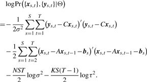Since the sequences of {x_s,t} are not observed, parameter estimation has to be done via maximizing the marginal log-likelihood logPr({y_s,t}|Θ).

It is widely believed that the biological network is not fully connected. Usual estimation via log likelihood does not lead to zero elements of network-related parameters A and {b_s}, which does not represent sparse networks. To obtain sparse solutions, we need to add some penalty terms to the marginal log-likelihood. In this article, we adopt the L₀ penalty term.

where χ is an indicator function and λ is a penalty coefficient to be determined in advance. How to decide the value of λ is an issue. We recommend 2 which corresponds to Akaike information criterion (AIC; Akaike, 1974), or log(NST) which corresponds to Bayesian information criterion (BIC; Schwarz, 1978), or a value close to them.

Another option is to add L₁ penalty term, which is computationally more tractable. However, in case of L₁ penalty, there is little suggestion on the choice of the trade-off parameter λ. Therefore, we adopt L₀ penalty at the expense of a little computational cost.

2.3.2 EM algorithm for the proposed model

Direct maximization of the marginal log-likelihood is intractable because it includes an integral term. Hence, we resort to the expectation-maximization (EM) algorithm. Although many studies (Ghahramani and Hinton, 1996; Roweis and Ghahramani, 1999) have adopted the EM algorithm for estimating parameters of state-space models, these methods are not applicable for the proposed model with the canonical cluster restriction. We newly derive a method for estimating parameters of our model. Further details are mentioned in the Supplementary Material.

2.4 Several remarks

2.4.1 Determination of the number of clusters

A major problem in cluster analysis is the estimation of the optimal number of clusters. Although a number of methods have been proposed (see, e.g. Krzanowski and Lai, 1988; Sugar and James, 2003; Tibshirani et al., 2001), none of the methods are considered decisive. Since the method of Krzanowski and Lai (1988) needs no resampling phases or hyperparameter selection, we use their approach with some modifications.

Let denote the estimated variance of noise in the observation model when the number of clusters is set to K, and then set

where,

We select K^*=arg max_KKL(K) as the optimal number of clusters. Note that, in the statistics used by Krzanowski and Lai (1988), and T × P are replaced by the sum of squares within clusters and the dimension number of data, respectively.

2.4.2 Split–merge procedure

Our approach, unfortunately, has the local minima problem, which is common to most clustering methods. One heuristic is to repeat optimizations with multiple initial values. In this article, we adopt a more sophisticated technique, a split–merge procedure, which is shown to be more effective than multiple initial values (Ueda et al., 2000).

In the split–merge procedure, two overlapping clusters are merged and one messy cluster is split at the same time, which can lead to a jump from ill-conditioned local minimas to better configurations. The detailed procedure is described in the Supplementary Material.

Thanks to this procedure, we can considerably avoid awkward local minimas without specially devised initialization strategies of model parameters. However, devising initialization may improve the procedure further especially when tackling complex problems with large number of clusters and stimuli.

2.4.3 Comparison with existing model-based clustering approaches

In many model-based clustering method for time-course gene expression data, it is assumed that the profiles of the cluster center [say, (x_k,1, x_k,2,…, x_k,T) in the setting of Section 2.1] are generated via some dynamic models such as an autoregressive (AR) model or a hidden Markov model (Ramoni et al., 2002; Wu et al., 2005). These assumptions of independence among individual profiles are not realistic since there obviously exists mutual interference among genes.

Our approach is also model-based clustering in the sense that a probabilistic model for temporal profiles is assumed. The difference is that the generative model in our method considers regulatory relationships among clusters, and Equation (6) represents those regulations. However, parameter estimation becomes slightly difficult when considering regulatory relationships.

3 NUMERICAL EXPERIMENTS ON SYNTHETIC DATA

In this section, we examine the following:

1. How the accuracy of network inference varies according to the number of stimulations?

2. The effectiveness of our method compared with those of the existing methods.

3.1 Experimental methodology

Synthetic data were generated as follows: the number of genes, clusters and time points were set as N = 200, K = 4 and T = 10, respectively. A total of 50 genes were allocated to each cluster. Changing the number of stimuli S from 1 to 5, we generated temporal profiles of genes according to the following model:

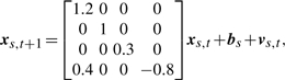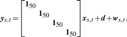where x_s,1=0, v_s,t ∼ N (0, (0.1)²I), 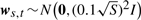and 1₅₀ is the 50-dimensional column vector whose elements are all 1. The term b_s corresponding to stimulations was set randomly at each trial as b_s ∼ N(0, (0.1)²I). The structure of this synthetic network is described in Figure 2. To secure the fairness in the number of experiments, we changed the variance of w_s,t, depending on the number of stimulations. When S reduces by half, we can have duplicate temporal profiles by carrying out the same number of experiments, which leads to a reduction of noise by .

Fig. 2.

The target cluster-based network for synthetic data.

We examined how the number of stimuli S and the penalty coefficient λ described in Section 2.3.1 influence the performance of network inference measured via sensitivity and specificity. These are defined as

where TP, TN, FP and FN are the number of true positive, true negative, false positive and false negative regulations, respectively. At the same time, we compared the clustering results with those of other popular methods, K-means with the Euclid distance and K-medoids method with the Pearson's correlation on the concatenated S T-dimensional vector {y_n,s,t}_{1≤s≤S,1≤t≤T} for each gene. For K-means and K-medoids, the best configuration of 300 repeats with respect to the corresponding loss function was chosen as the result for each trial. For measuring the accuracy of each clustering method, we used the number of genes allocated to wrong clusters. The penalty coefficient λ was changed over 1, 2, 4. The measures were averaged over 1000 randomly generated data.

3.2 Result

Tables 1–3 show the results. As S becomes larger, so does the dimension of parameters b_s that needs to be estimated. Furthermore the amount of noise increases according to S in this experimental setting. Nevertheless, both sensitivity and specificity rates improve as S becomes larger. Therefore, we can conclude that having temporal profiles with various types of stimuli is more helpful for inferring networks than having replicated temporal profiles with a single stimulation.

Table 1.

Sensitivity (%) versus the number of conditions

Method\the number of stimuli (s)	1	2	3	4	5
Proposed method (λ = 1)	78.45	91.83	96.45	98.42	99.20
Proposed method (λ = 2)	75.88	90.77	95.60	97.92	98.98
Proposed method (λ = 4)	62.22	85.32	93.47	96.03	98.18
K-means + DBN	6.58	24.42	37.35	46.80	52.75

Table 2.

Specificity (%) versus the number of conditions

Method\the number of stimuli (s)	1	2	3	4	5
Proposed method (λ = 1)	42.49	54.19	56.60	58.32	58.59
Proposed method (λ = 2)	61.75	69.83	72.94	73.45	74.56
Proposed method (λ = 4)	85.69	87.68	89.02	88.84	88.98
K-means + DBN	96.98	89.21	87.02	86.45	86.76

Table 3.

The number of misclassification for each method

Method\the number of stimuli (s)	1	2	3	4	5
K-means	24.71	3.08	2.63	0.97	0.15
K-medoids	30.87	18.00	21.01	24.33	25.53
Proposed method (λ = 1)	1.26	0.13	0.02	0.01	0
Proposed method (λ = 2)	1.26	0.12	0.02	0.01	0
Proposed method (λ = 4)	1.20	0.12	0.02	0.01	0

For a large λ, the sensitivity decreases whereas the specificity increases. Thus, λ should be adjusted according to usage: high λ leads to conservative inferences, while low λ tends to detect a large number of regulatory relationships.

With respect to clustering results, the proposed method is little affected by λ and is superior to K-means and K-medoids methods. As in the case of network inference, the clustering results become increasingly accurate as the number of stimulations increases.

Furthermore, we compared our approach with a clustering software TimeClust (Magni et al., 2008), which is designed specially for time-course gene expression data. We applied TimeClust only when S=1, since this method is not tailored to deal with multiple conditions. Using Bayesian clustering algorithm (Ferrazzi et al., 2005), which is implemented in this software, the average number of misclassification over 100 repeats is 11.04. This result shows the effectiveness of our approach compared with other advanced clustering methods for temporal gene expression profiles.

We also tested the network estimation result of the DBN with clustering using this dataset for comparison. We adopted K-means with 100 multiple initializations as a clustering method, and representative expression values on each cluster were changed into binary depending on positive or negative, to which DBN was applied. Multiple temporal profiles are treated as independent replicates. The optimal network was selected by maximizing BIC via simulated annealing. The results, which are shown in Tables 1 and 2, imply that our method is superior. When the number of stimulation conditions is large and λ=4, both sensitivity and specificity of our method are better than DBN.

4 COMPARISON TO AN EXISTING METHOD BASED ON STATE-SPACE MODELS

In this section, we compare the proposed method to the TRANS-MNET (Hirose et al., 2008), which is the software based on the state-space modeling.

Note that the purpose of our method is somewhat different from previous methods. Many previous approaches assume that each gene is associated with multiple state variables, and that each state variable is interpreted as a latent ‘module’, which represents the mechanism of gene regulation. One of the main goals of previous approaches including the TRANS-MNET is to extract such transcriptional modules that are considered to share common functions. On the other hand, our model is devised to cluster genes with similar temporal expression profiles imposing the role of a cluster on each state variable via the canonical cluster restriction.

4.1 Data

We adopted the time-course gene expression profile of Mus musculus circadian liver cells as experimental data, which is available at Gene Expression Omnibus (GEO, Accession number GSE3748). Samples were collected every 4 h for 48 h, for a total of 12 time points. We focused on 853 circadian genes, the list of which is available from Table 1 of the supporting information of Miller et al. (2007). Note that data under a single condition (S = 1) was selected because previous methods are not devised to deal with data under multiple conditions. The number of state variables K is set to 4 and 7.

4.2 Result

Figure 3 shows the profiles of state variables for both our method and the TRANS-MNET. In our method, all four profiles of cluster intermediates represent periodical processes with slightly different phases for K = 4. When K = 7, the number of profiles with periodical patterns increased to six. The heatmaps of the expression patterns of the genes are displayed in the Supplementary Figures 2 and 3. On the other hand, in the results of the TRANS-MNET, only two of four profiles of transcriptional modules showed clear cyclic patterns for both K = 4, 7. Therefore, at least for circadian rhythmic data, our method can capture periodical patterns more clearly than the TRANS-MNET can. For the clusters and modules extracted via our method and the TRANS-MNET, we performed the Gene Ontology (GO)-term enrichment analysis (see the Supplementary Table 4 for detailed results). However, there was no remarkable difference between the results of two methods.

Fig. 3.

Temporal profiles of cluster intermediates extracted via our method for K=4 (upper left) and K=7 (upper right). Temporal profiles of modules extracted via the TRANS−MNET for K=4 (lower left) and K=7 (lower right).

We do not claim that our method is superior in every way. There may be cases where several transcriptional modules governing the entire gene network exist and some genes belong to multiple modules. For such cases, the existing method may be more appropriate for extracting latent modules than our approach.

5 APPLICATION TO DIFFERENTLY STIMULATED MULTIPLE TIME-COURSE GENE EXPRESSION DATA

Epidermal growth factor (EGF) induces proliferation while heregulin (HRG) induces differentiation in MCF7 human breast cancer cells. Nagashima et al. (2007) identified 252 EGF- or HRG-regulated genes in early transcription. However, it is still unclear as to how these genes are linked to each other and function to determine cell fate. Since characterization of hundreds of genes is too large a task for detailed wet-lab experiments, capturing broad information via statistical methods is very helpful. Therefore, we applied the proposed method to this system.

5.1 Data

Cells were stimulated with 10 nM of either EGF or HRG for 0, 0.5, 1, 1.5, 2, 3, 4, 6 or 8 h. GeneChip (Affymetrix U133A version 2) experiments were performed, and the signals were processed according to robust multi-array average (RMA; Irizarry et al., 2003). We extracted 257 probe sets of the genes selected by Nagashima et al. (2007), and the expression profile of each gene was normalized so that the difference between the maximum and the minimum was 1 and the initial value was 0. (See Supplementary Table 1 for the list of probe sets used.) The penalty coefficient λ was set to 2.

5.2 Result

According to the procedure in Section 2.4.1, the number of clusters K was set to 6. The parameters A and b_s were estimated as follows:

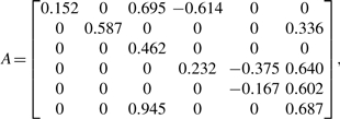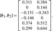where b₁ and b₂ represent the inferred regulations on clusters from EGF and HRG, respectively. Figure 4 shows the inferred network. See Supplementary Table 1 for genes in each cluster.

Fig. 4.

The inferred cluster-based network (self-regulations are omitted)

Figure 5 shows the temporal profiles of cluster intermediates. The heatmap of the expression patterns of the genes are displayed in the Supplementary Figure 1. Cluster 6 shows transient expression patterns for EGF and more prominently for HRG. The temporal profile of cluster 5 shows sustained expression patterns for both EGF and HRG. Most interestingly, the expression profile of cluster 2 moves up about an hour later after stimulation via HRG and is sustained for a while, whereas it remains static via stimulation via EGF.

Fig. 5.

Temporal profiles of cluster intermediates. Dashed lines represent temporal profiles for EGF whereas bold lines represent those for HRG. Error bars correspond to standard deviations of gene expression values on each time point

Estimated b₁ and b₂ show that regulations via EGF or HRG were inferred for most clusters, and their plus or minus (activation or inhibition) were found to be equal. However, except for cluster 4, HRG showed a stronger regulatory relationship (which can be measured via the absolute values) than EGF. These results are consistent with the argument of Nagashima et al. (2007) that EGF and HRG induce quantitative and not qualitative differences in transcriptional control, which determines the cell fate.

To evaluate the obtained network, we compared our results with the known regulatory relationships among genes. From the TRANSFAC database (Wingender et al., 2000), we extracted regulatory relationships among genes selected by Nagashima et al. (2007), which amounted to 19 regulatory relationships (see Supplementary Table 2). In 12 of them, both genes were included in the same cluster. In six of them, relationships were seen at the level of clusters. Therefore, our method successfully induced a reasonable network.

To verify our results with respect to the available biological knowledge, we performed the GO-term enrichment analysis for the set of genes in each cluster. Using the GOstat software (Beissbarth and Speed, 2004), for each cluster, we obtained the significance (P-value) of each GO term present in GO slims, which is the cut-down version of the whole GO. Significant GO terms were particularly observed in clusters 2, 3, 5 and 6. Detailed results are presented in the Supplementary Table 3.

A large number of transcription factor genes (ATF3, FOSL1, BHLHB2, JUNB, NR4A3, TSC22D2, FOS, KLF10, FOSB, DLX2, EGR2, EGR4, JUN, NR4A1, GATA6 and NR4A2) were aggregated in cluster 6 which is inferred to positively regulate clusters 2, 4 and 5. Although the functions of all the transcription factors in cluster 6 are not known, genes that encode the activator protein 1 (AP-1) transcription factor group that consist of FOS family proteins (c-FOS, FOSB, FRA-1/FOSL1 and FRA-2/FOSL2) and JUN family proteins (c-JUN, JUNB and JUND) are significantly involved in cluster 6. The AP-1 complex is activated by homo- and heterodimerization of the transcription factors, and mediates a wide range of biological effects related to cell growth, differentiation and cell death. On the other hand, regulated clusters 2 and 5 included many genes related to cell differentiation/death and development, respectively. Therefore, a given inferred network structure showing cluster six-regulated expression of clusters 2 and 5 seems to coincide with the expected function of the AP-1 complex.

However, no significant GO-term enrichment was observed in cluster 4, but MYC and RARA, which are believed to work as network hubs, were captured there. This observation is compatible with the fact that there are redundant regulatory functions related to cluster 4.

6 CONCLUSION

In this article, we propose a new statistical method for analyzing time-course gene expression data collected under multiple conditions. Although the probabilistic model assumed in our method is simple, we confirmed that our method can induce biologically important information. Furthermore, we verified using synthetic data that as the number of experimental conditions increases, the network estimation accuracy improves.

Note that many model-based methods assume some generative models considering the situation of interest. If multiple stimuli are not incorporated into the model, the method cannot deal with them. Methods which do not assume specific probabilistic models (e.g. K-means) are comparatively broadly applied in various situations such as multiple stimulation conditions. Nevertheless, we think model-based methods are beneficial because we can extract the nature of the data by investigating estimated parameters of the models. State-space model is not the only one suitable for dealing with multiple conditions. For example, we can make DBN so as to treat several different conditions by adding new nodes representing the existence of the stimuli.

To take advantage of differently stimulated multiple time-course expression data for inferring gene networks, wet-lab experimental designs must be carefully considered at the stage of collecting data. Furthermore, it is necessary to further elaborate the statistical method. Inferring gene networks is a very challenging project. We believe that collecting comparative temporal profiles collected under multiple stimulation conditions greatly facilitates this task.

REFERENCES

- Akaike H. A new look at the statistical model identification. IEEE Trans. Automat. Contr. 1974;19:716–723. [Google Scholar]
- Amit I, et al. A module of negative feedback regulators defines growth factor signaling. Nat. Genet. 2007;39:503–512. doi: 10.1038/ng1987. [DOI] [PubMed] [Google Scholar]
- Beal MJ, et al. A Bayesian approach to reconstructing genetic regulatory networks with hidden factors. Bioinformatics. 2005;21:349–356. doi: 10.1093/bioinformatics/bti014. [DOI] [PubMed] [Google Scholar]
- Beissbarth T, Speed TP. GOstat: find statistically overrepresented Gene Ontologies within a group of genes. Bioinformatics. 2004;20:1464–1465. doi: 10.1093/bioinformatics/bth088. [DOI] [PubMed] [Google Scholar]
- Bock C, Lengauer T. Computational epigenetics. Bioinformatics. 2008;24:1–10. doi: 10.1093/bioinformatics/btm546. [DOI] [PubMed] [Google Scholar]
- Bromberg KD, et al. Design logic of a cannabinoid receptor signaling network that triggers neurite outgrowth. Science. 2008;320:903–909. doi: 10.1126/science.1152662. [DOI] [PMC free article] [PubMed] [Google Scholar]
- Ferrazzi F, et al. Random walk models for Bayesian clustering of gene expression profiles. Appl. Bioinformatics. 2005;4:263–276. doi: 10.2165/00822942-200504040-00006. [DOI] [PubMed] [Google Scholar]
- Fraley C, Raftery AE. Model-based clustering, discriminant analysis, and density estimation. J. Am. Stat. Assoc. 2002;97:611–631. [Google Scholar]
- Ghahramani Z, Hinton GE. Technical report CRG-TR-96-2. Department of Computer Science, University of Toronto; 1996. Parameter estimation for linear dynamical systems. [Google Scholar]
- Harvey AC. Forecasting, structural time series models and the Kalman filter. New York: Cambridge University Press; 1989. [Google Scholar]
- Hirose O, et al. Statistical inference of transcriptional module-based gene networks from time course gene expression profiles by using state space models. Bioinformatics. 2008;24:932–942. doi: 10.1093/bioinformatics/btm639. [DOI] [PubMed] [Google Scholar]
- Imoto S, et al. Estimation of genetic networks and functional structures between genes by using Bayesian networks and nonparametric regression. Pacific Symposium on Biocomputing. 2002:175–186. [PubMed] [Google Scholar]
- Inoue LY, et al. Cluster-based network model for time-course gene expression data. Biostatistics. 2007;8:507–525. doi: 10.1093/biostatistics/kxl026. [DOI] [PubMed] [Google Scholar]
- Irizarry RA, et al. Exploration, normalization, and summaries of high density oligonucleotide array probe level data. Biostatistics. 2003;4:249–264. doi: 10.1093/biostatistics/4.2.249. [DOI] [PubMed] [Google Scholar]
- Kao S, et al. Identification of the mechanisms regulating the differential activation of the mapk cascade by epidermal growth factor and nerve growth factor in PC12 cells. J. Biol. Chem. 2001;276:18169–18177. doi: 10.1074/jbc.M008870200. [DOI] [PubMed] [Google Scholar]
- Kikuchi S, et al. Dynamic modeling of genetic networks using genetic algorithm and S-system. Bioinformatics. 2003;19:643–650. doi: 10.1093/bioinformatics/btg027. [DOI] [PubMed] [Google Scholar]
- Kim S, et al. Inferring gene networks from time series microarray data using dynamic Bayesian networks. Brief. Bioinform. 2003;4:228–235. doi: 10.1093/bib/4.3.228. [DOI] [PubMed] [Google Scholar]
- Kimura S, et al. Inference of S-system models of genetic networks using a cooperative coevolutionary algorithm. Bioinformatics. 2005;21:1154–1163. doi: 10.1093/bioinformatics/bti071. [DOI] [PubMed] [Google Scholar]
- Kimura S, et al. Genetic network inference as a series of discrimination tasks. Bioinformatics. 2009;25:918–925. doi: 10.1093/bioinformatics/btp072. [DOI] [PubMed] [Google Scholar]
- Krzanowski WJ, Lai YT. A criterion for determining the number of groups in a data set using sum-of-squares clustering. Biometrics. 1988;44:23–34. [Google Scholar]
- Luan Y, Li H. Clustering of time-course gene expression data using a mixed-effects model with B-splines. Bioinformatics. 2003;19:474–482. doi: 10.1093/bioinformatics/btg014. [DOI] [PubMed] [Google Scholar]
- Magni P, et al. TimeClust: a clustering tool for gene expression time series. Bioinformatics. 2008;24:430–432. doi: 10.1093/bioinformatics/btm605. [DOI] [PubMed] [Google Scholar]
- Martin S, et al. Boolean dynamics of genetic regulatory networks inferred from microarray time series data. Bioinformatics. 2007;23:866–874. doi: 10.1093/bioinformatics/btm021. [DOI] [PubMed] [Google Scholar]
- Miller BH, et al. Circadian and CLOCK-controlled regulation of the mouse transcriptome and cell proliferation. Proc. Natl Acad. Sci. USA. 2007;104:3342–3347. doi: 10.1073/pnas.0611724104. [DOI] [PMC free article] [PubMed] [Google Scholar]
- Miller-Jensen K, et al. Common effector processing mediates cell-specific responses to stimuli. Nature. 2007;448:604–608. doi: 10.1038/nature06001. [DOI] [PubMed] [Google Scholar]
- Nagashima T, et al. Quantitative transcriptional control of ErbB receptor signaling undergoes graded to biphasic response for cell differentiation. J. Biol. Chem. 2007;282:4045–4056. doi: 10.1074/jbc.M608653200. [DOI] [PubMed] [Google Scholar]
- Perrin BE, et al. Gene networks inference using dynamic Bayesian networks. Bioinformatics. 2003;19:138–148. doi: 10.1093/bioinformatics/btg1071. [DOI] [PubMed] [Google Scholar]
- Ramoni MF, et al. Cluster analysis of gene expression dynamics. Proc. Natl Acad. Sci. USA. 2002;99:9121–9126. doi: 10.1073/pnas.132656399. [DOI] [PMC free article] [PubMed] [Google Scholar]
- Rangel C, et al. Modeling T-cell activation using gene expression profiling and state-space models. Bioinformatics. 2004;20:1361–1372. doi: 10.1093/bioinformatics/bth093. [DOI] [PubMed] [Google Scholar]
- Roweis S, Ghahramani Z. A unifying review of linear Gaussian models. Neural Comput. 1999;11:305–345. doi: 10.1162/089976699300016674. [DOI] [PubMed] [Google Scholar]
- Sachs K, et al. Causal protein-signaling networks derived from multiparameter single-cell data. Science. 2005;308:523–529. doi: 10.1126/science.1105809. [DOI] [PubMed] [Google Scholar]
- Schwarz G. Estimating the dimension of a model. Ann. Stat. 1978;6:461–464. [Google Scholar]
- Segal E, et al. Learning module networks. J. Mach. Learn. Res. 2005;6:557–588. [Google Scholar]
- Sugar CA, James GM. Finding the number of clusters in a dataset: an information-theoretic approach. J. Am. Stat. Assoc. 2003;98:750–763. [Google Scholar]
- Tibshirani R, et al. Estimating the number of clusters in a data set via the gap statistic. J. R. Stat. Soc. Ser. B. 2001;63:411–423. [Google Scholar]
- Toh H, Horimoto K. Inference of a genetic network by a combined approach of cluster analysis and graphical Gaussian modeling. Bioinformatics. 2002;18:287–297. doi: 10.1093/bioinformatics/18.2.287. [DOI] [PubMed] [Google Scholar]
- Ueda N, et al. SMEM algorithm for mixture models. Neural Comput. 2000;12:2109–2128. doi: 10.1162/089976600300015088. [DOI] [PubMed] [Google Scholar]
- Wingender E, et al. TRANSFAC: an integrated system for gene expression regulation. Nucleic Acids Res. 2000;28:316–319. doi: 10.1093/nar/28.1.316. [DOI] [PMC free article] [PubMed] [Google Scholar]
- Wu FX, et al. Dynamic model-based clustering for time-course gene expression data. J. Bioinform. Comput. Biol. 2005;3:821–836. doi: 10.1142/s0219720005001314. [DOI] [PubMed] [Google Scholar]
- Yamaguchi R, et al. Finding module-based gene networks with state-space models - mining high-dimensional and short time-course gene expression data. IEEE Signal Process. Mag. 2007;24:37–46. [Google Scholar]
- York RD, et al. Role of phosphoinositide 3-kinase and endocytosis in nerve growth factor-induced extracellular signal-regulated kinase activation via Ras and Rap1. Mol. Cell. Biol. 2000;20:8069–8083. doi: 10.1128/mcb.20.21.8069-8083.2000. [DOI] [PMC free article] [PubMed] [Google Scholar]
- Zhong S, Ghosh J. A unified framework for model-based clustering. J. Mach. Learn. Res. 2003;4:1001–1037. [Google Scholar]
- Zou M, Conzen SD. A new dynamic Bayesian network (DBN) approach for identifying gene regulatory networks from time course microarray data. Bioinformatics. 2005;21:71–79. doi: 10.1093/bioinformatics/bth463. [DOI] [PubMed] [Google Scholar]
Associated Data
This section collects any data citations, data availability statements, or supplementary materials included in this article.