Helix-Sheet Packing in Proteins

Abstract

The three-dimensional structure of a protein is organized around the packing of its secondary structure elements. While much is known about the packing geometry observed between α-helices and between β-sheets, there has been little progress on characterizing helix-sheet interactions. We present an analysis of the conformation of αβ₂ motifs in proteins, corresponding to all occurrences of helices in contact with two strands that are hydrogen-bonded. The geometry of the αβ₂ motif is characterized by the azimuthal angle θ between the helix axis and an average vector representing the two strands, the elevation angle ψ between the helix axis and the plane containing the two strands, and the distance D between the helix and the strands. We observe that the helix tends to align to the two strands, with a preference for an antiparallel orientation if the two strands are parallel; this preference is diminished for other topologies of the β-sheet. Sidechain packing at the interface between the helix and the strands is mostly hydrophobic, with a preference for aliphatic amino acids in the strand and aromatic amino acids in the helix. From the knowledge of the geometry and amino acid propensities of αβ₂ motifs in proteins, we have derived different statistical potentials that are shown to be efficient in picking native-like conformations among a set of non-native conformations in well-known decoy datasets. The information on the geometry of αβ₂ motifs as well as the related statistical potentials has applications in the field of protein structure prediction.

1 Introduction

In 1951, Pauling and Corey published a series of theoretical papers on the structure of proteins that became famous as the ”protein papers” ^1-7. The studies that were reported established the importance of protein structures for the biologists and this understanding has since only grown. Discovering all genes in various genomes and their relationship to proteins has become a priority since the middle of the 1990s, leading to the genomics projects: currently, there are over seven million protein sequences in the UniPro-tKB/TrEMBL database⁸. In parallel and in line with the ”protein papers”, large scale studies of protein structures have been developed under the structural genomics projects. Finding the structure of a protein however is a much more demanding task than finding its sequence: currently, only about 60,000 structures solved by experimental methods are available in the PDB, the repository of protein structures ^9,10. Computer-based protein structure prediction is highly regarded as a complement to experimental studies that will help close this knowledge gap between sequence and structure. Success of existing methods for structure prediction is monitored regularly through a series of experiments, the biannual Critical Assessment of Structure Prediction (CASP) meetings ¹¹. These meetings have highlighted the importance of the knowledge extracted from the known protein structures that can serve as direct templates for homology-based prediction or as data to derive general rules on protein structures. Among the latter, packing of secondary structures has probably attracted the most attention, as it is seen as an intermediate step between the knowledge of the sequence and the structure of a protein. In this paper, we focus on one of these geometric packing, namely the packing between helices and strands.

In their ”protein papers”, Pauling and Corey described proteins as a 3D assembly of regular elements, which they refer to as the α-helix and the β-strand, with the second organized in a series of β-sheets. The first high resolution X-ray structures of proteins confirmed their prediction ^12-14; these structures also revealed the absence of predictable symmetry in the arrangement of these secondary structures, henceforth complicating the chance that the structure of a protein can be predicted ab initio. However, as early as 1976 and based on 31 protein structures only, Levitt and Chothia ¹⁵ observed that secondary structures do not pack randomly. They introduce the concept of classes which divides proteins into four different groups :all α, all β, α/β and α + β for proteins comprised of helices only, strands and sheets only, alternating helices and strands, and mixture of helices and strands, respectively. Today, the number of structures in the PDB is larger than 60,000. Levitt and Chothia's observations remain mainly valid: the geometry of secondary structure packing is biased towards a few conformations, as described in detail in the existing protein structure classification: SCOP ¹⁶, CATH ¹⁷ and FSSP ¹⁸. This gives us hope that if we can understand and even predict this bias, we will be close to solving the protein structure prediction problem.

Most protein structures contain a mixture of helices and sheets ^16,17; as these structures are tightly packed, it is therefore expected that contacts between these two types of secondary structure occur frequently. The most famous example of such a contact is found in the βαβ fold in which the helix that connects the two parallel strands is tightly packed against the β sheet. There are many other types of α helix / β sheet packing, however, in which the helix and the sheet are located in different parts of the sequence. The geometries that result from the packing of α helices on a β sheet have been studied in details about thirty years ago, by thorough analysis of the few protein structures known at the time ^15,19-21. These studies have been regularly updated ^22-25 as well as complemented with computational studies of the stability of helix-sheet motifs ²⁶. They usually agree that the most favorable arrangement of an helix packed on a β-sheet has the axis of the helix oriented along the strands of the sheet, as a result of attractive sidechain - sidechain interactions. If the two strands are parallel in the β-sheet, it is also found that the helix axis aligns anti-parallel to the sheet axis ²⁵. Another energetically favorable packing, albeit less frequently observed, sees the helix axis being perpendicular to the strands ^23,26. Based on an analysis of 141 well resolved structures, Boutonnet and colleagues ²³ have shown that in fact the helix packs on the sheet with virtually all relative orientations, with the parallel and perpendicular positions being preferred. The helix - sheet packing is usually further characterized by two other geometric measures, i.e. the elevation angle between the plane defined by the sheet and the helix axis, and the distance between the sheet and the helix. The former is usually found to be around 0, i.e. the helix is parallel to the plane, while the latter is found to be around 10 Å^15,21.

This study updates the analyses presented above. We analyze the packing between α-helices and β-sheets observed in all αβ₂ motifs with the two β strands forming a sheet in a database of 6729 non-redundant, high resolution protein structures and derive rules that are translated into statistical potentials. We show that the geometry of these motifs is not random and that the bias observed can be used to score the quality of protein models. The paper is organized as follows. In the next section, we describe the different classes of αβ₂ subunits found in proteins, as well as the geometric measures we use to characterize them. In the results section, we show the distribution of these geometric measures for the different classes. We further derive statistical potentials from these distributions and test them on well-established decoy datasets. We conclude the paper with a discussion on the application of these results to protein structure prediction.

2 Method

2.1 Database of protein structures

To analyze and evaluate the αβ₂ motifs found in protein structures, we have built a database of high resolution, non redundant proteins for which the structures are available in the PDB database. This database is constructed as follows. First, we include all proteins from the PDB that do not share more than 90 % sequence identity (this set is derived from the PDB by performing a search without keyword and setting the sequence filter at 90 % percent). Second, we remove all structures whose resolution is worse than 2 Å . Using the PDB stamped September 2008, our database contains 6729 protein chains.

2.2 The αβ₂ motif

Previous studies of helix-sheet packing have focused on the interaction between one single helix and one single strand or between a helix and a pleated sheet. However, many native structures show that one helix can interact with more than one strand within the same sheet. In this study, we focus on the αβ₂ subunit that contains one helix in contact with two strands that are hydrogen bonded to each other to form a sheet. This definition covers a wide range of configurations. For example, the helix can be before, in between or after the two strands in the protein sequence. In addition, the two strands need not be directly sequential, i.e. there can be other strands between them along the sequence. We identify the αβ₂ motifs of a protein using the following procedure. First, we use STRIDE²⁷ to detect all helices and strands in the protein structure. Second, we check for contacts between each helix and each strand, where contact means that the minimal distance between any two atoms belonging to their respective side chains is less than 4Å. When a helix is found to be in contact with two strands that form a sheet, it defines an αβ₂ subunit which is subsequently stored. Using this procedure, we extracted 31,949 αβ₂ motifs from our protein structure database. Note that two different motifs in this database may share the same helix or the same β sheet, but obviously not both.

2.3 Geometric measures for αβ₂ motifs

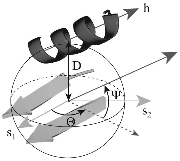
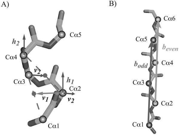
The packing between the helix and the two strands in an αβ₂ subunit is characterized by two angles, θ and ψ and one distance, D, as illustrated in Figure 1. The α-helix and β-strands are represented as vectors, referred to as the helix and strand axes (see figure 2 for a geometric definition of these two axes). We require that helices and strands contain at least four and three residues, respectively. In each αβ₂ subunit, there are one helix represented with its h vector and two strands represented with their b₁ and b₂ vectors. The indices refer to the precedence of the two strands along the protein sequence, with strand 1 and strand 2 being close to the N and C termini, respectively. The average vector s₁ representing the sheet formed by the two strands is defined as s₁ = b₁ + b₂ where addition and subtraction correspond to the strands being parallel or antiparallel, respectively.

Figure 1. Illustration of the geometric measures characterizing a αβ₂ unit.

The position of the helix is defined with respect to a co-ordinate system anchored on the β-sheet. s₁ is the mean vector representing the two strands, while s₂ is a vector perpendicular to s₁ in the plane containing the sheet. The orientation of the helix axis h is defined according to a polar co-ordinate system: the azimuthal angle θ is the angle between s₁ and the projection of h in the plane defined by s₁ and s₂, while the elevation angle ψ is the angle between this plane and h. D measures the distance between the helix and the sheet (see text for details).

Figure 2. Geometric definitions of the axes of a helix and of a strand.

A) The axis h of an helix is computed in two steps. First, a local axis is derived for each four consecutive residues that belong to the helix. For the four residues whose Cαs are Cα1, Cα2, Cα3 and Cα4, the local helix axis h₁ is given by h₁ = v₁ × v₂, where × is the cross-product, v₁ is the vector from Cα2 to the mid-point between Cα1 and Cα3, and v₂ is the vector from Cα3 to the middle of Cα2 and Cα4. Second, the axis of the helix is set to the average of all its local axes. B) The axis b of a strand is set to be the average of the two local axes b_odd and b_even corresponding to its odd and even residues, respectively. The local axis b_odd corresponds to the direction of the line of best fit over all odd C_αs in the strand (i.e. in positions 1,3,… where the index of the first residue in the strand is 1). A similar definition is used for the even axis b_odd.

We also compute the least square plane 𝒢 defined by the C_α atoms of the residues that are hydrogen-bonded in the sheet formed by the two strands. s₂ is the vector perpendicular to s⃗₁ in that plane. The angle θ is the azimuthal angle, i.e. the angle between s₁ and the projection of h in the plane 𝒢, while the angle ψ is the angle between the vector h and the plane 𝒢 (ψ is often referred to as the elevation angle). D is the average of the distances between all C_α atoms in the helix and the plane 𝒢. Using θ, ψ and D, we are able to describe the relative position of a helix to a local sheet; we investigate whether there are biases on these three geometric measures of helix-sheet packing in native proteins.

2.4 Classification of αβ₂ units

An αβ₂ unit contains three elements that can be arranged with different topologies that account for the direction of the strands in the sheet (parallel or antiparallel) as well as for the relative position of the helix with respect to the two strands. We define four different patterns for an αβ₂ unit; each pattern is identified with a label of the form PiTj, with both i and j ∈ 0,1, defined as follows:

• i relates to the relative orientation of the two strands; it is set to 0 if the two β strands are antiparallel, and 1 otherwise.

• j relates to the relative position of the helix and the strands in the protein sequence; it is set to 1 if the two strands are sequential and the helix is sandwiched between them along the sequence, and 0 otherwise, e.g. there is another strand between two paired strands or the helix is before/after the two strands in the sequence.

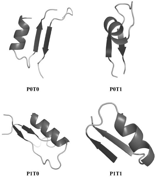
Figure 3 shows one representative for each of the four motif types (P0T0, P0T1, P1T0, P1T1) extracted from native protein structures.

Figure 3. Representatives of the four different patterns of αβ₂ units in proteins.

The P0T0, P0T1, P1T0, and P1T1 example units are extracted from proteins 1VQ1(A226-249), 2O1N(116-145), 1COZ(1-28), and 2P7H(A21-46) respectively. P indicates if the two strands are parallel or antiparallel to each other, while T relates to the relative position of the strands and the helix along the protein sequence. Figure drawn with Pymol.

2.5 Propensities of amino acid types at the helix-strand interface

We compute the propensity that a residue type i in a helix is found at the interface between this helix and one of the strands in an αβ₂ motif using:

$$P_H\left(i\right)=\frac{P^{\mathit{helix},I}\left(i\right)}{P^{\mathit{helix}}\left(i\right)}$$ (1)

where P^helix,I(i) is the probability that an amino acid of type i in a helix belongs to a helix-strand interface and P^helix(i) is the probability of finding amino acid type i in an helix. P^helix(i) is computed using:

$$P^{\mathit{helix}}\left(i\right)=\frac{N_i}{N}$$ (2)

where N is the total number of residues found in helices of the αβ₂ motifs considered, and N_i is the number of those residues that are of type i. Similarly, P^helix,I(i) is computed using:

$$P^{\mathit{helix},I}\left(i\right)=\frac{N_i^I}{N^I}$$ (3)

where N^I is the total number of residues found in helices that are part of an interface, and N_i is the number of those residues that are of type i.

A similar expression is used to compute P_S(i).

In parallel, we compute the propensity of finding a residue pair with type (i,j) at the interface between the helix and one of the two strands in an αβ₂ motif according to the following definition:

$$P(i,j)=\frac{1}{M}\frac{M_{\mathit{ij}}}{P^{\mathit{helix}}\left(i\right)P^{\mathit{strand}}\left(j\right)}$$ (4)

where i and j refers to the types of the residues in the helix and in the strand, respectively and M is the total number of residue pairs considered. M_ij is the number of residue pairs of type (i, j) at the interface, P^helix(i) and P^strand(j) are the probability of finding residue types i and j in an helix and a strand, respectively. P^helix(i) is computed using equation 2; a similar equation is used for computing P^strand(i). Note that P(i,j) is a propensity: if its value is greater than one, a contact between residue types i and j is favored, while if its value is smaller than one, this contact is less frequent than a random model would predict.

2.6 Scoring a protein based on the geometry of its αβ₂ motifs

We score a protein that contains one or more αβ₂ motifs using the regularity of their geometric measures as well as the bias in the type of amino acid contacts they contain.

Firstly, three different geometric scores are computed. Each αβ₂ motif is characterized by its azimuthal and elevation angles θ and ψ, respectively, and by its helix-strand distance D (see above). The score assigned to each parameter is the log of the frequency at which its measure is observed in our database of native αβ₂ motifs:

$$S_X\left(\mu \right)=-\log \left(\frac{P(X=\mu )}{P_U(X-\mu )}\right)$$ (5)

where X is any of the three properties θ, ψ or D, μ is the value found in the motif of interest, P is the probability distribution function derived from the database of natif motifs, and P_U is a reference uniform probability distribution function.

Secondly, we derive a score based on the propensities of amino acids at the interface between the helix and the strands of the αβ₂ motif. We start by listing all pairs of residues that participate in this interface. A pair (i,j) where i and j are the amino acid types for the residues belonging to the helix and to the strand, respectively, contributes to the total score:

$$S_{\mathit{pair}}(i,j)=-\log \left(P(i,j)\right)$$ (6)

where P(i,j) is the propensity defined in equation 4. We assume that the pairs of residues in the interface are independent of each other. Using the product rule for probabilities that converts to a sum rule for their logarithm, the score of the interface is the sum of the scores of all pairs in the interface.

Note that we use in both cases the log of the probabilities to make the scores additive: if the protein contains several αβ₂ motifs, its score is the sum of the individual scores of the motifs.

3 Results

We study the geometry of αβ₂ motifs in proteins, as well as the sequence specificity of helix-strand contacts within such motifs. From a non redundant database of high resolution protein structures (see method), we extract 31, 949 αβ₂ motifs which we divide into four groups, based on the orientation of the two strands in the sheet (P1 if the strands are parallel and P0 otherwise), and the relative position of the helix with respect to the strands (T1 if the helix is in between the two strands along the protein sequence, and T0 otherwise). The four corresponding groups, P0T0, P0T1, P1T0 and P1T1 contain 15492, 291, 11632 and 4534 motifs, respectively.

3.1 Geometry of αβ₂ motifs

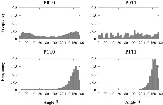
The relative position of the helix in the αβ₂ motif with respect to the sheet formed by the two strands is characterized by three geometric measures, two angles θ and ψ and one distance D. Figures 4, 5 and 6 show the distributions of these three measures over all motifs included in our database, and divided according to the four groups defined above.

Figure 4.

The distributions of angle θ defining the azimuthal angle between the axis and the plane of the β sheet in a αβ₂ motif See text and Figure 3 for a definition of the four sub-classes of the motifs.

Figure 5.

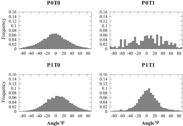
The distributions of angle ψ defining the elevation angle between the axis of the helix and the plane containg the β sheet in a αβ₂ motif. See text and Figure 3 for a definition of the four sub-classes of the motifs. All four distributions are centered on 0°, corresponding to the helix being parallel to the plane containing the two strands.

Figure 6.

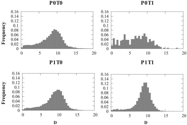
The distributions of distance D defining the mean separation between the axis of the helix and the plane containing the β sheet in a αβ₂ motif See text and Figure 3 for a definition of the four sub-classes of the motifs.

The angle θ measures the relative orientation between the axis of the β sheet and the projection of the axis of the helix on the plane containing the β sheet (equivalent to the azimuthal angle in polar coordinates). Figure 4 shows the distributions of θ for the four subgroups P0T0, P0T1, P1T0 and P1T1. If the two strands in the sheet are parallel to each other (P1), the distributions of θ values are found to be uni-modal, with a sharp peak centered at θ = 165°. Clearly, a helix in contact with two parallel strands forming a β sheet is usually found to be parallel to the two strands, with its axis running antiparallel to the direction of the strands. The distribution of θ values for helices packed on strands forming an antiparallel β-sheet differs significantly from those observed for parallel β-sheets (panels P0T0 and P0T1 versus P1T0 and P1T1 in figure 4. In the most general case in which the helix is not sandwiched between the two strands (panel P0T0), the distribution is found to be bi-modal, with optimal values for θ = 15° and θ = 165°. Note that in this case, the presence of two peaks is an artifact of our definition of θ. We define the direction of the β sheet as the difference of the two vectors representing the axes of the two strands. While these two vectors are mostly parallel and define a direction s⃗₁, the orientation of their difference along s⃗₁ is arbitrary and depend on the order in which these two strands appear in the protein sequence. If we do not account for this orientation issue, the axis of an helix in contact with two antiparallel strands is preferably 15° away from the mean axis of the two strands. The situation is different if the helix is sandwiched between the two strands along the sequence of the protein. While there are not many motifs that fall in this category, the distribution of θ for these motifs is found to be nearly uniform.

The angle ψ is the elevation angle between the β sheet plane and the helix axis. Figure 5 shows the distributions of ψ for all four types of αβ₂ motifs. In opposition to the distributions of θ angles that show significant differences when comparing these four types, the distributions of ψ are much more similar. All four are uni-modal, centered on 0°, i.e. with the axis of the helix parallel to the plane containing the β sheet.

The measure D estimates the distance between the helix and the plane 𝒢 containing the β sheet of a motif αβ₂. As the helix may be tilted with respect to the plane, D is set as the average distance between all C_α atoms in the helix and 𝒢. Figure 6 shows the distribution of D for the four subgroups of αβ₂ motifs. All four distributions are uni-modal, with a maximum around 9 Å, with more than 70 % of the motifs in the range [8,12]. Note again that the distribution for the group P0T1 (i.e. antiparallel sheet with the helix sandwiched between the two strands along the sequence) is not as regular, mostly as the sample size is much smaller.

3.2 Favored residues found at α helix - β strand interfaces

We computed the propensites P_H(i) and P_S(i) that a residue of type i in an helix and a strand, respectively, belongs to the helix-strand interface of an αβ₂ motif for all twenty types of amino acids, over all motifs in our database. Results are given in table 1. The log of the propensity is given instead of the propensity itself; as such, a value of 0 indicates that the actual propensity is 1, meaning that the amino acid i is found to be preferentially in the interface, while positive and negative values indicate positive and negative bias, respectively. We find that these propensities are very similar between helices and strands. In both types of secondary structures, hydrophobic as well as aromatic residues are found preferentially at the interface, while polar residues are usually not observed at the interface.

Table 1.

Propensities of amino acids to be in an α-β interface

Amino Acid	Helix (log(PH)) a	Strand (log(PS ))
GLY	−0.16	−0.13
ALA	−0.19	−0.17
VAL	0.36	0.16
ILE	0.53	0.44
LEU	0.49	0.31
PHE	0.87	0.60
PRO	−0.88	−0.40
MET	0.45	0.14
TRP	0.71	0.30
CYS	−0.34	−0.78
SER	−0.33	−0.61
THR	0.10	−0.50
ASN	−0.68	−0.39
GLN	−0.64	−0.77
TYR	0.45	0.38
HIS	−0.06	−0.16
ASP	−0.86	−0.43
GLU	−0.92	−0.70
LYS	−0.96	−1.04
ARG	−0.52	−0.56

^aP_H is the propensity that an amino acid of type i in a helix sits at the interface between this helix and a strand in an αβ₂ motif (see equation 1). The log of P_H is given, such that positive values indicate that this residue type is favored at he interface, while negative values indicate that this residue type is rarely seen as part of the interface.

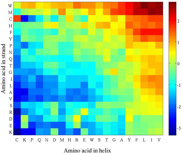
We also computed the propensities P(i,j) of finding a residue of type i in the helix of a αβ₂ motif to be in contact with a residue of type j in one of the two strands of the motif for all 400 possible type pairs, over all motifs in our database. Results are shown in figure 7. Clearly, there are preferred types of contacts, involving mostly hydrophobic residues. Valine, Leucine, Isoleucine, Phenylalanine in helices are often found at the interface, with a preference to be in contact with an aromatic residue (Tryptophan, Phenylalanine, Tyrosine or Histidine) or with a Methionine or a Cysteine. A cysteine in a helix makes little contact with residues in a strand, except if this residue is a cysteine in which case they form a disulphide bridge. Note that the contact matrix is not symmetric: it is interesting for example that a cysteine, a methionine or a tryptophan in a strand has more contacts with different residue types in helices than a cysteine, a methionine or a tryptophan in a helix has contacts with residues in strands.

Figure 7.

Log of the propensities of finding a contact of type (i, j) at the interface between a helix and a strand in an αβ₂ motif. For clarity of presentation, amino acids on the rows and columns of this matrix are ordered based on contact similarity as follows. Each amino acid type is characterized by a twenty dimensional vector (for example a column in the contact matrix). These vectors are used to compute a similarity matrix that is given as input to a metric multi dimensional scaling (MDS) algorithm ⁴³. The latter assigns a position to each amino acid type in a 1D space and these positions define the ordering of the columns of the contact matrix. The same procedure is used to order the rows.

3.3 Statistical potentials based on αβ₂ motifs

We have shown that αβ₂ motifs in proteins adopt specific conformations that can be described by three geometric measures, i.e. the azimuthal (θ) and elevation (ψ) angles that specify the position of the helix with respect to the β sheet plane, and the distance D between the helix and the sheet. In addition, we have shown that the residues at the interface have non-random types. Here we assess how it is possible to use these properties to distinguish native-like models of proteins from non-native conformations. We use three geometric scores, S_θ, S_ψ, and S_D and one propensity score S_P on twenty decoy sets (see table 2 for a list of the proteins). Complete results for the decoy set 4ubpA are shown in figure 9 while summary results for the twenty decoy sets are provided in table 2.

Table 2.

Correlation coefficients between score S and RMSD for twenty standard decoy sets

Decoy set	PDB id	S θ	S ψ	S D	S pair
Rosetta a	4ubpA	0.55	0.65	0.38	0.46
Rosetta	2acy	0.45	0.74	0.48	0.57
Rosetta	1aiu	0.60	0.46	0.69	0.57
Rosetta	1ew4	0.60	0.71	0.65	0.72
Rosetta	1ughI	0.26	0.41	0.57	0.51
Rosetta	1kpeA	0.12	0.45	0.37	0.54
Rosetta	1fkb	−0.11	0.48	0.66	0.04
Rosetta	1bm8	0.24	0.10	0.10	0.30
Rosetta	2chf	0.55	0.07	0.45	0.45
Rosetta	1dhn	0.18	0.50	0.51	0.39
Rosetta	1ptq	0.78	0.54	−0.45	0.01
Rosetta	1scjB	−0.09	0.46	0.57	0.50
Rosetta	1a19A	0.45	−0.68	0.68	0.29
Rosetta	1cc8A	−0.18	0.52	0.34	0.58
lmds b	2ovo	0.08	0.16	0.36	0.65
lmds	1igd	0.28	0.23	0.08	0.11
4state c	1sn3	0.38	0.18	0.29	−0.03
4state	4pti	0.22	−0.08	−0.20	−0.07
lattice ssfit d	1pgb	0.73	0.12	0.61	−0.02
semfold e	1khmA	0.01	−0.42	−0.14	−0.07

^aAll atom decoy sets from Rosetta@home, available at http://depts.washington.edu/bakerpg/decoys/

^bAll atom decoy sets from Keasar and Levitt ⁴⁴

^cAll atom decoy sets from Park and Levitt ⁴⁵

^dAll atom decoy sets from Xia et al ⁴⁶

^eAll atom decoy set from Samudrala and Levitt ⁴⁷

The four decoy sets lmds, 4 state. lattice ssfit and semfold are available from the Decoys ‘R’ us repository ²⁹.

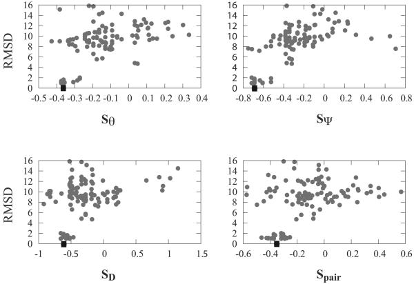
Figure 9. Score-RMSD scattered plots for the 4ubpA decoy set analysed with four statistical potentials specific to their αβ₂ motifs.

These four potentials capture the azimuthal angle between the helix and strands (θ), the elevation angle between the plane containing the sheet and the helix (ψ), the distance D between the helix and the sheet, and the propensity of the aminoacid pairs in the interface between the helix and the strands (PR). In all four panels, the native protein is shown as a square.

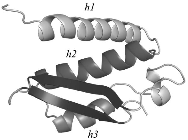
4ubp is the name of the PDB file containing the high resolution X-ray structure (R = 1.55 Å) of an urease from Bacillus Pasteurii. Chain A of 4ubp is a small globular domain of 100 residues, whose structure belongs to the α + β class, with one antiparallel β-sheet and three helices. Two of these helices are packed on the β-sheet, forming two αβ₂ motifs, both in the P0T0 class (see figure 8 for details). The structure of 4ubpA was predicted using Rosetta²⁸ and a set of 130 models with low Rosetta scores is available in the Rosetta decoy set. We have scored these 130 models using all four statistical potentials mentioned above; results are shown in figure 9. The two geometric scores based on θ and ψ angles, as well as the pairwise potential that scores the interface between the helix and the strands perform best. Note that for all four potentials, the native structure does not have the lowest (most favorable) score.

Figure 8. Cartoon representation of the native structure of chain A of the urease 4ubp.

The central antiparallel β sheet (in blue) defines two αβ₂ motifs, the first one involving the helix h2 (residues 31-49), the second one involving the helix h3 (residues 52-61). Figure drawn with Pymol.

An ideal statistical potential would identify the native conformation with the lowest (more favorable) score and rank all the other conformations according to their RMS distance to the native structures. In practice, the quality of a potential is often defined according to the correlation between scores and RMS distances. If the potential is designed such that favorable scores have low values, positive correlations above 0.7 are considered good, while small correlation values or even negative values indicate that it is not detecting differences between native-like and wrong models. Table 2 gives the correlation coefficients between the four scores that are specific to αβ₂ motifs and RMS for twenty different decoys. These decoys come from two main sources: the Rosetta decoys from the David Baker's laboratory and the repository of protein decoys Decoys ‘R’ us ²⁹. They were chosen for their contents in αβ₂ motifs. Note that a decoy structure is scored only if it contains at least one motif that satisfies our definition of the αβ₂ motif. Clearly, none of the four potentials can be considered as being consistently good. For all four potentials, the near-native decoys have low (favorable) scores. Results differ however for the decoy structures that deviate significantly from the native conformation. In some of the test cases (such as 4ubpA and 1ptq using the potential S_θ, 4ubpA, 2acy and 1ew4 using the potential S_ψ or 1aiu and 1a19A using S_D), the RMSD distance between the decoy and the native protein correlates well with the score; in other cases (see for example the panel corresponding to S_D in figure 9), the scores appear unrelated to the RMSD values. While these levels of performance are at best similar and often lower than those observed with other statistical potentials ³⁰, these results remain encouraging. The four potentials tested here only ascertain the quality of the geometry of the αβ₂ motifs in the protein as well as the nature of the interface between the helix and the strands; the fact that potentials specific to these motifs perform well on decoy sets indicate that these motifs are central to the overall geometry of the protein structure.

4 Discussion

4.1 Conserved structure features in αβ₂ motifs

Our structural analysis of 31,949 αβ₂ motifs in proteins reveals that while nearly all geometries are possible, some arrangements of the secondary structures are more frequently observed than others, in agreement with previous observations ^{15,23,25,26,31} We characterize the geometry of a αβ₂ motif with three geometric measures, the azimuthal angle θ between the axis of the sheet formed by the two strands and the projection of the helix axis on the plane containing the sheet, the elevation angle ψ between this plane and the helix axis, and the distance D between the plane and the axis.

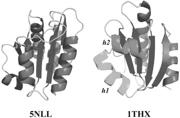
The most common arrangement sees the helix mostly aligned to the two strands, with a strong preference to be anti-parallel if the two strands are parallel (θ close to 180°); this preference is diminished if the two strands are anti-parallel (see figure 4). The same feature has been observed previously on much smaller datasets. Chothia and colleagues had proposed already in 1977 that a helix is packed onto a sheet with its axis parallel to the strands ¹⁵. This arrangement was explained based on favorable geometry for the side-chain packing. It was later confirmed on a much larger set of motifs ²³ as well as by computational experiments ²⁶. In addition, Hespenheide and Kuhn observed that helices tend to be aligned antiparallel to parallel β-sheets, and that this tendency is diminished for helices that are packed on antiparallel β-sheets ²⁵. However, the aligned arrangement of the helix and the strands is not unique. Using energy computations, Chou et al ²⁶ observed that a class with a nearly perpendicular orientation of the helix axis to the strands is also of low energy. Boutonnet et al ²³ confirmed that such perpendicular arrangements are found in αββ and ββα motifs in which the helix is located either before or after two consecutive strands in the sequence of the proteins, albeit not as frequent as the parallel arrangement. On a much larger set of motifs, we observe that perpendicular packing of the helix on the strands is quite rare on parallel strands, more frequent if the two strands are antiparallel and as favorable as any other orientation if in addition the helix is sandwiched between the two strands. More generally, the difference between motifs containing parallel and anti-parallel strands is observed for many possible orientations of the helix: while the presence of parallel strands usually implies that the helix is antiparallel to the strands, anti-parallel strands are more permissive. Figure 10 illustrates this difference in two native proteins.

Figure 10. Different packing styles observed in αβ₂ motifs in proteins.

5NLL (left panel), abacterial flavodoxin is a small protein of 138 residues formed of a parallel β-sheet with 5 strands surrounded by 5 helices. 5NLL contains 9 αβ₂ motifs (8 within the P1 T0 category, and 1 in the P1T1 category), all with parallel strands. In all these motifs, the angle θ is close to 170°. 1THX (right panel), a theoredoxin is another small αβ protein whose structure includes an anti-parallel β-sheet covered with 3 helices, forming 6 αβ₂ motifs, two with parallel strands and 4 with antiparallel strands. Note that 1THX contains a fourth helix (shown in green) that does not participate in any of the αβ₂ motifs. The three helices present different orientation with respect to the sheet: helix 2 for example (shown in magenta) is perpendicular to the two strands it is packed on. Figure drawn with Pymol.

The two other geometric measures that describe a αβ₂ motif are much less informative. The helix in αβ₂ motifs is found to be on average parallel to the plane containing the β-sheet (ψ = 0) and 10 Å away from that plane, independent of the motif type (see figures 5 and 6). These values are quite intuitive and express a compromise between the definition of a motif that imposes contacts between the helix and the strands and the steric constraints that prevent side-chains to overlap. It is well known for example that the average distance between the axes of two packed helices as well as the distance between β-sheets and between a β-sheet and a helix is typically 10 Å. Taylor has applied this general property to represent proteins on a ideal lattice and to use these ideal forms to predict the structures of proteins ^32,33.

Finally, note that we have considered here ideal conformations for the helix and the strands: we do not take into account the fact that the helix may be bent and that the strands are twisted. While these are important properties of the individual secondary structures, we do not believe that they affect our understanding of the geometry of αβ₂ motifs in proteins.

4.2 Amino acid propensity at the helix-strand interface

The concept of amino acid propensities for secondary structures was introduced and put into use for prediction in the 1970s by Chou and Fassman ³⁴. These early studies based on the small set of proteins available at the time have been continuously updated and improved as the size of the PDB was increasing. The accuracy of secondary structure prediction based on these propensities has reached however a limit that is usually assigned to the inability of this model to account for long range effects. The importance of the environment was recently emphasized by Costantini et al who showed that amino acid propensities for secondary structures differ in different structural classes ³⁵. We have shown here that helix-strand packing in αβ₂ motifs results in preferred sidechain interactions that may explain these differences. To further investigate this effect, we plan to study the difference in the propensities of amino acids in helix-strand and helix-helix packing.

Not surprisingly, the contacts between helices and strands are mostly hydrophobic, with cysteine-cysteine disulphide bridges being the only notable exception. Interestingly however, the amino acid preferences in helix and strands are not symmetric: aliphatic, hydrophobic amino acids dominate on the helix side, while aromatic amino acids dominate on the strand side. The reason for this difference is unclear at this time.

4.3 Scoring protein models based on their αβ₂ motifs

Statistical potentials, also referred to as mean field potentials or knowledge-based potentials, are “energies” that are widely used for protein structure prediction. While physics-based potentials rely on first principles, these potentials are derived from observed properties in databases of protein structures. The most common statistical potential measures the “normality” of the amino acid pairwise contacts occuring in a protein structure, where normality refers to the expectancy derived from known native structures. Other properties however have been translated into statistical potentials, such as angle measures, solvent accessibility and hydrogen bond characteristics (for review, see 36). In this paper, we have derived three geometry-based and one frequency-based statistical potentials specific to αβ₂ motifs and applied these potentials to score different decoy sets. Our results are surprisingly good: in most decoy tests and for all four potentials native-like structural models have low, favorable scores while decoys whose structures significantly differ from the native structure have high scores. In addition, there is a good correlation between the score and the RMS distance over the whole range of decoy structures. While these results are not perfect (they are many statistical potentials that perform better on these decoys, see for example Summa et al. ³⁰), they are very encouraging as the statistical potentials we have introduced analyze only the αβ₂ motifs present in the structure.

Questions on the validity of statistical potentials have been raised several times (see for example Thomas and Dill ³⁷). Their derivation is based on many assumptions and approximations, such as statistical independence that are not always satisfied. Our derivation is pragmatic and ignores these hidden problems. In some sense, we have developed statistical potentials on a highly biased database that only contains αβ₂ motifs. The database dependence of statistical potentials has been studied before ^38,39. These studies have shown that potentials derived from specialized databases perform better than those derived from generic databases, when applied on proteins that relate to the former. The results presented here are akin to those.

4.4 Applications to protein structure prediction

The most common approach for protein structure prediction proceeds in two steps. A large set of models is constructed for the protein of interest; these models are then assessed using a scoring function, and the conformations with the most favorable scores are assumed to be native like. The results presented in this work suggest two applications, one for each of these steps. Firstly, we have established consensus conformations for different classes of αβ₂ motifs, depending on the relative orientation of the two strands (parallel or anti-parallel) as well as on the relative position of the helix with respect to the two strands in the protein sequence. These consensus conformations can serve as scaffold for generating models of the protein of interest, with correct local geometry. This approach parallels the approach of Taylor and co-workers who defined a “periodic table” for protein structures ³² containing a set of ideal conformation for proteins that are subsequently used to generate thousands of models for the protein of interest ³³. A similar approach was used by Baker and co-workers for strand-loop-strand motifs ^40,41. Secondly, the statistical potentials presented here may be used to score the different models generated for a given protein. Note that we suggest these scores as compreplements and not alternatives to existing scores. Note also that the statistical scores based on the geometry of the αβ₂ motif become redundant if the consensus motifs were used to generate the models; the pairwise potential that scores the interface between the helix and the strand remains however useful. We are currently working on implementing both approaches in ProteinShop, a general platform for protein structure analysis and prediction ⁴².

References

- 1.Pauling L, Corey R. Atomic coordinates and structure factors for two helical configurations of polypeptide chains. Proc. Natl. Acad. Sci. (USA) 1951;37:235–240. doi: 10.1073/pnas.37.5.235. [DOI] [PMC free article] [PubMed] [Google Scholar]
- 2.Pauling L, Corey R. The structure of synthetic polypeptides. Proc. Natl. Acad. Sci. (USA) 1951;37:241–250. doi: 10.1073/pnas.37.5.241. [DOI] [PMC free article] [PubMed] [Google Scholar]
- 3.Pauling L, Corey R. The pleated sheet, a new layer configuration of polypeptide chains. Proc. Natl. Acad. Sci. (USA) 1951;37:251–256. doi: 10.1073/pnas.37.5.251. [DOI] [PMC free article] [PubMed] [Google Scholar]
- 4.Pauling L, Corey R. The structure of feather rachis keratin. Proc. Natl. Acad. Sci. (USA) 1951;37:256–261. doi: 10.1073/pnas.37.5.256. [DOI] [PMC free article] [PubMed] [Google Scholar]
- 5.Pauling L, Corey R. The structure of hair, muscle, and related proteins. Proc. Natl. Acad. Sci. (USA) 1951;37:261–271. doi: 10.1073/pnas.37.5.261. [DOI] [PMC free article] [PubMed] [Google Scholar]
- 6.Pauling L, Corey R. The structure of fibrous proteins of the collagen-gelatin group. Proc. Natl. Acad. Sci. (USA) 1951;37:272–281. doi: 10.1073/pnas.37.5.272. [DOI] [PMC free article] [PubMed] [Google Scholar]
- 7.Pauling L, Corey R. The polypeptidechain configuration in hemoglobin and other globular proteins. Proc. Natl. Acad. Sci. (USA) 1951;37:282–285. doi: 10.1073/pnas.37.5.282. [DOI] [PMC free article] [PubMed] [Google Scholar]
- 8.Bairoch A, Bougueleret L, Altairac S, Amendolia V, Auchincloss A, Puy G, Axelsen K, Baratin D, Blatter M, Boeckmann B, et al. The universal protein resource (UniProt) 2009. Nucleic Acids Res. 2009;37:D169–D174. doi: 10.1093/nar/gkn664. [DOI] [PMC free article] [PubMed] [Google Scholar]
- 9.Bernstein F, Koetzle T, Williams G, Jr EM, Brice M, Rodgers J, Kennard O, Shimanouchi T, Tasumi M. The Protein Data Bank: a computer-based archival file for macromolecular structures. J. Mol. Biol. 1977;112:535–542. doi: 10.1016/s0022-2836(77)80200-3. [DOI] [PubMed] [Google Scholar]
- 10.Berman H, Westbrook J, Feng Z, Gilliland G, Bhat T, Weissig H, Shindyalov I, Bourne P. The Protein Data Bank. Nucleic Acids Res. 2000;28:235–242. doi: 10.1093/nar/28.1.235. [DOI] [PMC free article] [PubMed] [Google Scholar]
- 11.Moult J. A decade of CASP: progress, bottlenecks and prognosis in protein structure prediction. Curr. Opin. Struct. Biol. 2005;3:285–289. doi: 10.1016/j.sbi.2005.05.011. [DOI] [PubMed] [Google Scholar]
- 12.Kendrew J, Bodo G, Dintzis H, Parrish R, Wyckoff H, Phillips D. A three-dimensional model of the myoglobin molecule obtained by x-ray analysis. Nature. 1958;181:662. doi: 10.1038/181662a0. [DOI] [PubMed] [Google Scholar]
- 13.Kendrew J, Dickerson R, Strandberg B, Hart R, Davies D. The structure of myoglobin: a three-dimensional fourier synthesis and 2å resolution. Nature. 1960;185:422–427. doi: 10.1038/185422a0. [DOI] [PubMed] [Google Scholar]
- 14.Blake C, Koenig D, Mair G, North A, Phillips D, Sarma V. Structure of hen egg-white lysozyme. a three-dimensional fourier synthesis at 2 angstroms resolution. Nature. 1965;206:757–61. doi: 10.1038/206757a0. [DOI] [PubMed] [Google Scholar]
- 15.Chothia C, Levitt M, Richardson D. Structure of proteins: packing of α-helices and pleated sheets. Proc. Nat. Acad. Sci. (USA) 1977;74:4130–4134. doi: 10.1073/pnas.74.10.4130. [DOI] [PMC free article] [PubMed] [Google Scholar]
- 16.Murzin AG, Brenner SE, Hubbard T, Chothia C. Scop: a structural classification of proteins database for the investigation of sequences and structures. J. Mol. Biol. 1995;247:536–540. doi: 10.1006/jmbi.1995.0159. [DOI] [PubMed] [Google Scholar]
- 17.Orengo C, Michie A, Jones D, Swindells M, Thornton J. CATH: A hierarchic classification of protein domain structures. Structure. 1997;5:1093–1108. doi: 10.1016/s0969-2126(97)00260-8. [DOI] [PubMed] [Google Scholar]
- 18.Holm L, Ouzounis C, Sander C, Tuparev G, Vriend G. A database of protein structure families with common folding motifs. Protein Sci. 1992;1:1691–1698. doi: 10.1002/pro.5560011217. [DOI] [PMC free article] [PubMed] [Google Scholar]
- 19.Sternberg M, Thornton J. On the conformation of proteins: the handedness of the beta-strand alpha-helix beta-strand helix. J. Mol. Biol. 1976;105:367–382. doi: 10.1016/0022-2836(76)90099-1. [DOI] [PubMed] [Google Scholar]
- 20.Richardson J. Handedness of crossover connections in beta sheets. Proc. Nat. Acad. Sci. (USA) 1976;73(8):2619–2623. doi: 10.1073/pnas.73.8.2619. [DOI] [PMC free article] [PubMed] [Google Scholar]
- 21.Cohen F, Sternberg M, Taylor W. Analysis and prediction of the packing of alpha-helices against a beta-sheet in the tertiary structure of globular proteins. J. Mol. Biol. 1982;156:821–862. doi: 10.1016/0022-2836(82)90144-9. [DOI] [PubMed] [Google Scholar]
- 22.Reddy BVB, Blundell TL. Packing of secondary structural elements in proteins: Analysis and prediction of inter-helix distance. J. Mol. Biol. 1993;233:464–479. doi: 10.1006/jmbi.1993.1524. [DOI] [PubMed] [Google Scholar]
- 23.Boutonnet N, Kajava A, Rooman M. Structural classification of αββ and ββα supersecondary structure units in proteins. Proteins: Struct. Func. Genet. 1998;30:193–212. [PubMed] [Google Scholar]
- 24.Reddy B, Nagarajaram HA, Blundell T. Analysis of interactive packing of secondary structural elements in α/β units in proteins. Protein Sci. 1999;8:573–586. doi: 10.1110/ps.8.3.573. [DOI] [PMC free article] [PubMed] [Google Scholar]
- 25.Hespenheide B, Kuhn L. Discovery of a significant, nontopological preference for antiparallel alignment of helices with parallel regions in sheets. Protein Sci. 2003;5:1119–1125. doi: 10.1110/ps.0238803. [DOI] [PMC free article] [PubMed] [Google Scholar]
- 26.Chou K, Nemethy G, Rumsey S, Tuttle RW, Scheraga H. Interactions between an alpha-helix and a beta-sheet. energetics of alpha/beta packing in proteins. J. Mol. Biol. 1985;186:591–609. doi: 10.1016/0022-2836(85)90133-0. [DOI] [PubMed] [Google Scholar]
- 27.Frishman D, Argos P. Knowledge-based secondary structure assignment. Proteins: Struct. Func. Genet. 1995;23:566–579. doi: 10.1002/prot.340230412. [DOI] [PubMed] [Google Scholar]
- 28.Simons K, Bonneau R, Ruczinski I, Baker D. Ab initio protein structure prediction of CASP III targets using ROSETTA. Proteins. 1999;3(Suppl. 3):171–176. doi: 10.1002/(sici)1097-0134(1999)37:3+<171::aid-prot21>3.3.co;2-q. [DOI] [PubMed] [Google Scholar]
- 29.Samudrala R, Levitt M. Decoys ‘R’ us: A database of incorrect protein conformations to improve protein structure prediction. Protein Sci. 2000;9:1399–1401. doi: 10.1110/ps.9.7.1399. [DOI] [PMC free article] [PubMed] [Google Scholar]
- 30.Summa C, Levitt M, DeGrado WF. An atomic environment potential for use in protein structure prediction. J. Mol. Biol. 2005;352:986–1001. doi: 10.1016/j.jmb.2005.07.054. [DOI] [PubMed] [Google Scholar]
- 31.Platt D, Guerra C, Zanotti G, Rigoutsos I. Global secondary structure packing angle bias in proteins. Proteins Struct. Funct. Genet. 2003;53:252–261. doi: 10.1002/prot.10448. [DOI] [PubMed] [Google Scholar]
- 32.Taylor W. A periodic table for protein structures. Nature. 2000;416:457–460. doi: 10.1038/416657a. [DOI] [PubMed] [Google Scholar]
- 33.Taylor WR, Bartlett G, Chelliah V, Klose D, Lin K, Sheldon T, Jonassen I. Prediction of protein structure from ideal forms. Proteins Struct. Funct. Genet. 2008;70:1610–1619. doi: 10.1002/prot.21913. [DOI] [PubMed] [Google Scholar]
- 34.Chou P, Fasman G. Prediction of protein conformation. Biochemistry. 1974;13:222–245. doi: 10.1021/bi00699a002. [DOI] [PubMed] [Google Scholar]
- 35.Costantini S, Colonna G, Facchiano A. Amino acid propensities for secondary structures are influenced by the protein structural class. Biochem. Biophys. Research Comm. 2006;342:441–451. doi: 10.1016/j.bbrc.2006.01.159. [DOI] [PubMed] [Google Scholar]
- 36.Shen M-Y, Sali A. Statistical potential for assessment and prediction of protein structures. Protein Sci. 2006;15:2507–2524. doi: 10.1110/ps.062416606. [DOI] [PMC free article] [PubMed] [Google Scholar]
- 37.Thomas P, Dill K. Statistical potentials extracted from protein structures: how accurate are they? J. Mol. Biol. 1996;257:457–469. doi: 10.1006/jmbi.1996.0175. [DOI] [PubMed] [Google Scholar]
- 38.Furuichi E, Koehl P. Influence of protein structure databases on the predictive power of statistical pair potentials. Proteins: Struct. Func. Genet. 1998;31:139–149. doi: 10.1002/(sici)1097-0134(19980501)31:2<139::aid-prot4>3.0.co;2-h. [DOI] [PubMed] [Google Scholar]
- 39.Zhang C, Liu S, Zhou H, Zhou Y. The dependence of all-atom statistical potentials on structural training database. Biophys. J. 2004;86:3349–3358. doi: 10.1529/biophysj.103.035998. [DOI] [PMC free article] [PubMed] [Google Scholar]
- 40.Ruczinski I, Kooperberg C, Bonneau R, aker D. Distributions of beta sheets in proteins with application to structure prediction. Proteins. 2002;48:85–97. doi: 10.1002/prot.10123. [DOI] [PubMed] [Google Scholar]
- 41.Kuhn M, Meiler J, Baker D. Strand-loop-strand motifs: prediction of hairpins and diverging turns in proteins. Proteins. 2004;54:282–288. doi: 10.1002/prot.10589. [DOI] [PubMed] [Google Scholar]
- 42.Crivelli S, Kreylos O, Hamann B, Max N, Bethel W. ProteinShop: a tool for interactive protein manipulation. J. Comput. Aided Molec. Des. 2004;18:271–285. doi: 10.1023/b:jcam.0000046822.54719.4f. [DOI] [PubMed] [Google Scholar]
- 43.Cox T, Cox M. Multidimensional Scaling. Chapman and Hall/CRC; Baton Roca,FL: 2001. [Google Scholar]
- 44.Keasar C, Levitt M. A novel approach to decoy set generation: Designing a physical energy function having local minima with native structure characteristics. J. Mol. Biol. 2003;329:159–174. doi: 10.1016/S0022-2836(03)00323-1. [DOI] [PMC free article] [PubMed] [Google Scholar]
- 45.Park B, Levitt M. Energy functions that discriminate x-ray and near native folds from well-constructed decoys. J. Mol. Biol. 1996;258:367–392. doi: 10.1006/jmbi.1996.0256. [DOI] [PubMed] [Google Scholar]
- 46.Xia Y, Huang E, Levitt M, Samudrala R. Ab initio construction of protein tertiary structures using a hierarchical approach. J. Mol. Biol. 2000;300:171–185. doi: 10.1006/jmbi.2000.3835. [DOI] [PubMed] [Google Scholar]
- 47.Samudrala R, Levitt M. A comprehensive analysis of 40 blind protein structure predictions. BMC Struct. Biol. 2002;2:3–18. doi: 10.1186/1472-6807-2-3. [DOI] [PMC free article] [PubMed] [Google Scholar]