A Novel Wavelet-based Thresholding Method for the Pre-processing of Mass Spectrometry Data that Accounts for Heterogeneous Noise

Abstract

In recent years there has been an increased interest in using protein mass spectroscopy to discriminate diseased from healthy individuals with the aim of discovering molecular markers for disease. A crucial step before any statistical analysis is the pre-processing of the mass spectrometry data. Statistical results are typically strongly affected by the specific pre-processing techniques used. One important pre-processing step is the removal of chemical and instrumental noise from the mass spectra. Wavelet denoising techniques are a standard method for denoising. Existing techniques, however, do not accommodate errors that vary across the mass spectrum, but instead assume a homogeneous error structure. In this paper we propose a novel wavelet denoising approach that deals with heterogeneous errors by incorporating a variance change point detection method in the thresholding procedure. We study our method on real and simulated mass spectrometry data and show that it improves on performances of peak detection methods.

1 Introduction

In recent years applications of protein mass spectrometry (MS) technologies in biomedical research have flourished. Popular technologies to produce MS data include surface-enhanced laser desorption/ionization time-of flight mass spectrometry (SELDI-TOF MS) and matrix-assisted laser desorption/ionization time-of-flight mass spectrometry (MALDI-TOF MS). Broadly speaking, a mass spectrum plots the time-of-flight on the x-axis and ion counts on the y-axis. Alternatively, time-of-flight can be transformed to molecular weight over charge (m/z) and ion counts into a signal intensity. Peaks constitute the most important features of a single spectrum. In proteomic studies the goal is often to identify peaks related to specific outcomes, such as different malignancies or clinical responses. Proteins corresponding to the selected peaks can then be identified via additional experimental work.

Mass spectrometry data consist of tens of thousand measurements and are inherently noisy. Major sources of noise stem from interference from the matrix material and sample contaminations (chemical noise) and the physical characteristics of the machine (electrical noise), [1, 2, 3]. Typically, pre-processing is done before any statistical analysis and includes baseline subtraction, denoising, normalization, peak detection, and peak alignment. The quality of the results of any subsequent statistical analysis heavily depends on these pre-processing steps, and especially on the denoising. Several denoising algorithms employing wavelet techniques have been developed, see for example Coombes et al. [4], Qu et al. [5] and Randolph and Yasui [6].

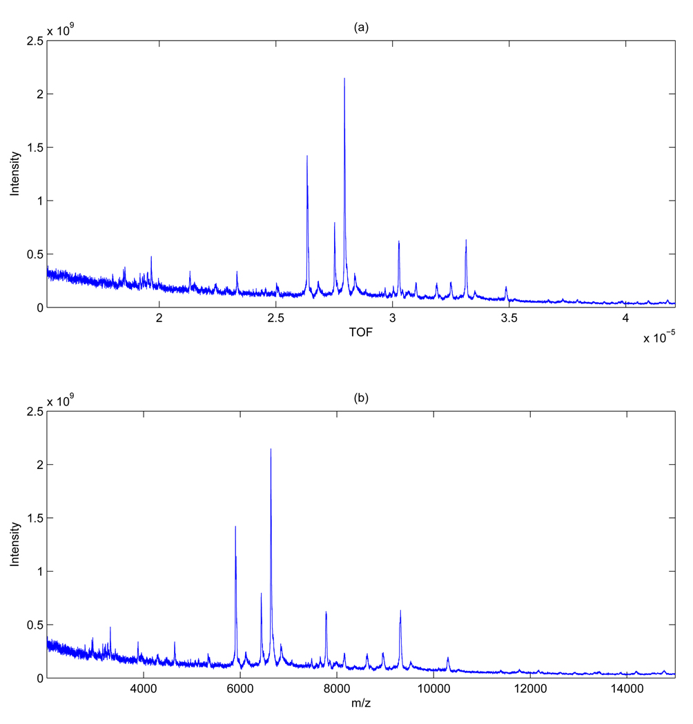
Our work is motivated by the observation that noise in MS data is mainly generated by chemical and electrical influences that tend to affect different m/z ranges differently. Experimental factors that contribute to this noise variation include laser inefficiency and spatial differences in total protein and matrix material content, i.e. inhomogeneity of the sample. Figure 1 displays the SELDI-TOF spectrum of a cancer patient collected for a biomarker discovery study on ovarian cancer (see Section 3.1 for details) and clearly shows that the noise component affects the lower m/z range more strongly. Heterogeneous noise can also be observed in Figure 1 of Coombes et al. [4]. These plots support our motivation for a denoising procedure that takes into account the heteroscedasticity of the noise. Most of the existing procedures for MS data, however, assume homoschedastic noise accross the m/z range. One exception is the work of Chen et al. [7] who accommodates heteroscedastic noise by applying a global thresholding procedure to segments of the data, with the number of segments determined by the user.

Figure 1.

Ovarian cancer data: Plots of one MS spectrum in the time domain (a) and m/z domain (b).

Here we propose a novel wavelet denoising method that makes use of a variance change point detection algorithm to accommodate the heteroscedasticity of noise in the MS data. Our method is a block-thresholding procedure that first identifies change points in the variance of the data and then applies wavelet thresholding locally by computing the threshold values based on segments identified by the change points. For the location of the variance change points we use an iterated cumulative sums of squares (ICSS) algorithm adapted to wavelet packets, as recently proposed by Gabbanini et al. [8]. We then divide the wavelet coefficients into subintervals identified by the change points and compute local thresholds. We show that, when applied to SELDI-TOF MS data from an ovarian cancer discovery study, our local denoising procedure leads to improved subsequent performances of peak detection algorithms. We also assess performance of our procedure on simulated data.

The rest of the paper is organized as follows. Section 2 briefly discusses the proposed procedure that achieves local wavelet thresholding by employing methods for variance change point detection. In Section 3 we demonstrate our approach on ovarian cancer MS data and we explore its performance on simulated data. We close the paper with a discussion in Section 4. The technical details about the wavelet transforms and the variance change detection algorithm are described in the supplementary material and the Appendix at the end of the paper.

2 Methods

We first describe our procedure for local wavelet thresholding of MS data. Details of the methods are left to the Appendix and supplementary material.

2.1 Wavelet Denosing

Wavelets are families of orthonormal bases that can be used to parsimoniously represent functions. Following the seminal work of Donoho and Johnstone [9, 10], wavelet thresholding has successfully been used in various applications to remove noise and recover the true signal. This is accomplished by applying a wavelet transform to the data and then mapping wavelet coefficients that fall below a threshold to 0 (hard thresholding) or shrinking all coefficients toward 0 (soft thresholding). One can also opt between a global or an adaptive thresholding rule. The former applies the same threshold, i.e. identical cut-off value, to all wavelet coefficients, whereas the latter uses a threshold that depends on the resolution level of the wavelet transform. An inverse wavelet transform is then applied to the thresholded coefficients, leading to a smoothed estimate of the signal.

For mass spectrometry data, both traditional discrete wavelet transforms (DWT), see Mallat [11], and undecimated tranforms, such as the maximal overlap discrete wavelet transform (MODWT) of Percival and Walden [12], have been used, see Coombes et al. [4] and Kwon et al. [13]. When using undecimated coefficients, hard thresholding has better denoising performance. A commonly used thresholding rule is the universal global threshold of Donoho and Johnstone, defined as

$$\mathrm{\lambda }=\widehat{\sigma }\sqrt{2\text{log}n},$$ (1)

where the estimate σ̂ of the noise standard deviation is computed based on the median absolute deviation (MAD) of the coefficients at the finest level of the wavelet transform

$$\widehat{\sigma }=\sqrt{2}\text{MAD}/.6745,$$ (2)

where MAD = median(|w−median(w)|) and w the vector of wavelet coefficients at the finest level. Coombes et al. [4] investigated performances of global thresholds of the type λ = C × σ̂ with C a user-defined constant that depends on the data to be analyzed. Here we also investigate the modification proposed by [14] to accomodate data contaminated by correlated noise, which amounts to use level-dependent thresholds of the type

$${\mathrm{\lambda }}_j={\widehat{\sigma }}_j\sqrt{2\text{log}n}$$ (3)

where ${\widehat{\sigma }}_j=\sqrt{2}\text{median}(|{\mathbf{w}}_j-\text{median}({\mathbf{w}}_j)|)/.6745$ with w_j the vector of wavelet coefficients at level j.

2.2 Local Thresholding Algorithm

We work with raw, un-processed, MS data. The first step of our local thresholding procedure identifies the location of change points in the variance of the data. The procedure is based on the iterated cumulative sums of squares algorithm of Inclan and Tiao [15] for the location of variance changes in a set of uncorrelated observations. This procedure was adapted to wavelet decompositions of long memory data by Whitcher et. al. [16] and generalized to short-memory data and to wavelet packets by Gabbanini et al. [8]. A binary segmentation of the data allows the procedure to detect multiple change points. The procedure can be applied to any pattern of variance changes. The details of the procedure are given in the Appendix.

Having found the locations of the variance change points, we then proceed by applying wavelet thresholding locally, by estimating the noise variance in the different segments identified by the variance changes. We use universal thresholds of type (1), i.e.,

$${\mathrm{\lambda }}_s={\widehat{\sigma }}_s\sqrt{2\text{log}{n}_s}$$ (4)

where n_s is the number of wavelet coefficients that belong to segment s and σ̂_s the estimate of the noise standard deviation in the same segment. We also investigate level-dependent thresholds of type (2), i.e.,

$${\mathrm{\lambda }}_j^s={\widehat{\sigma }}_{j,s}\sqrt{2\text{log}{n}_s}$$ (5)

with σ̂_j,s the estimate of the noise standard deviation at level j in segment s.

We now summarize the proposed local wavelet thresholding procedure step by step.

1. Compute the wavelet transforms of the data. In this paper we got better qualitative denoising with undecimated transforms over standard decimated discrete wavelet transforms. These transforms do not impose restrictions on the length of the data points and are shift-invariant, i.e., they are not affected by the starting position of the signal. We therefore used maximum overlap discrete wavelet transforms (MODWT). We also recommend Daubechies’ wavelets with 3 to 4 vanishing moments. See Section 3.3. for additional discussion.

2. Test for presence of variance change points by applying the ICSS algorithm (see Appendix) based on the discrete wavelet packet transforms (DWPT) coefficients. For the results here reported we used the Ljung-Box test with lag 10 in order to identify the wavelet packet to which apply the ICSS test. The procedure does not require any other user-defined parameter. For the variance change test we recommend to choose a fixed significance level of α = 0.01. If the null hypothesis (no variance change) is rejected, the locations of the variance change points can then be found using the maximal overlap discrete wavelet packet transforms (MODWPT) coefficients.

3. Divide the maximal overlap discrete wavelet transforms (MODWT) coefficients in segments according to the locations at which variance changes have been detected.

4. Compute a local threshold value for each segment using either equation (4) or equation (5).

5. Threshold the wavelet coefficients by hard or soft thresholding rule. For the data analysed in this paper we obtained satisfactory results by thresholding the finest four levels.

6. Reconstruct the denoised signal by inverse wavelet transform.

3 Data Examples

We briefly describe the SELDI-TOF MS data from an ovarian cancer biomarker discovery study and compare the performances of the proposed wavelet denoising method with the standard algorithm of Coombes et al. [4] that uses a global threshold. We then present results on simulated MS data.

3.1 Ovarian Cancer Data

Serum samples from women diagnosed with ovarian cancer and women hospitalized for other conditions, collected at the Mayo Clinic between 1980 and 1989, were analyzed by surface-enhanced laser desorption and ionization time-of-flight (SELDI-TOF) mass spectrometry using the CM10 chip type [17]. The ProteinChip Biomarker System (Ciphergen Biosystems) was used for protein expression profiling. Serum samples were analyzed by scientists blinded to disease status at Ciphergen Biosystems. A detailed description of the samples and exclusion criteria can be found in Moore et al. [18].

Similarly to an earlier analysis, Kwon et al. [13], we used the 50 samples obtained after 1986, whose serum was freeze-thawed a single time. For this paper we used the raw data, i.e, the actual ion counts measured on the time-of-flight (TOF) scale. We discarded m/z values lower than 2,000, due to very large noise, and m/z values greater than 15,000, because all the intensities in this range were very low. We applied wavelet thresholding to the data in the time-of-flight (TOF) domain, since the raw intensities obtained from the detector are taken at evenly spaced time intervals (in micro-seconds) in such domain.

In Figure 1, we plot one raw mass spectrum in both time and m/z domain. The conversion between TOF and m/z is based on the equation $\frac{m/z}{U}=\mathit{\text{sign}}(t-t_0)·a·{(t-t_0)}^2+b$, where t denotes time of flight, U = 25, 000, a = 3.36E8 , b = 0.00235, and t₀ = 3.7071E − 7. A single spectrum has 21, 551 data points.

3.2 Wavelet Denoising for ovarian cancer data

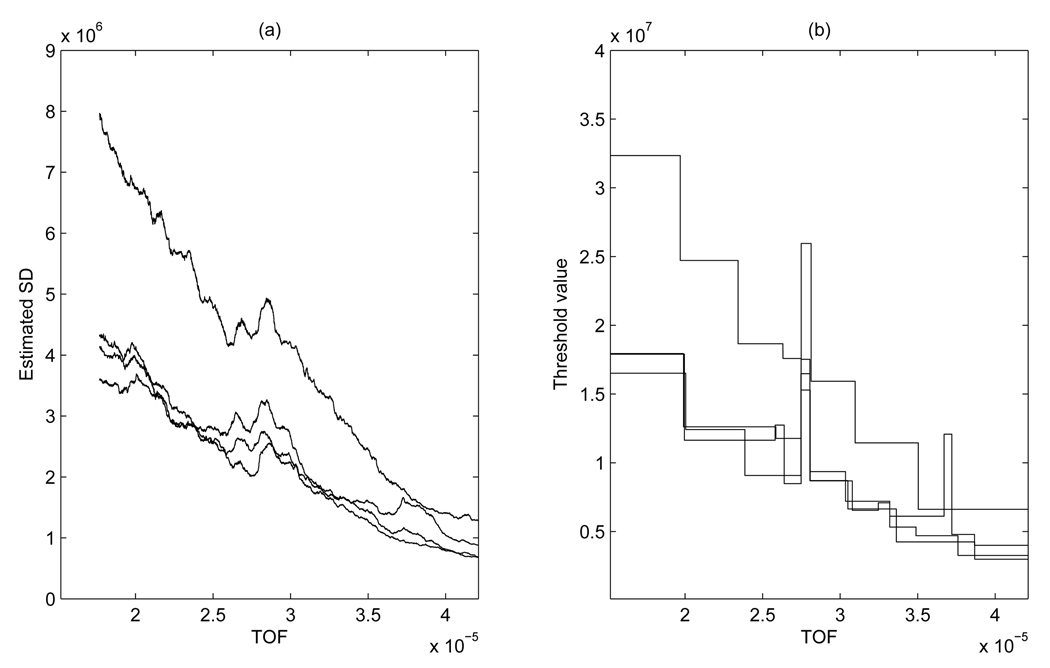
A closer look reveals the heterogeneous nature of the data collected in this study. This is clearly visible in Figure 1, as already highlighted in Section 1, and supported by Figure 2 (a), which displays estimated standard deviations of the noise for four randomly chosen spectra. These estimates were obtained by running an MAD smoother with window size 1,500 on the finest MODWT coefficients and show a clear decreasing trend as the TOF values increase. Figure 1 and Figure 2 indicate, in particular, that the high frequency components of the spectrum reduce in variance as the TOF values increase. With such noise pattern, standard schemes for wavelet thresholding result either in under-smoothness in the small TOF range or in over-smoothness in the large TOF range. For illustrative purposes, Figure 2 (a), shows the corresponding threshold values λ_s of type (4) calculated on segments of the data corresponding to the locations of the variance change points identified by our procedure. Similar plots can be obtained with the level-dependent thresholds of type (5). It appears that the threshold values approximate the estimated SD’s with a piecewise constant curve. The observed percent change in the threshold value over the 2,000–15, 000 m/z range varies between 78% and 82% for the four spectra.

Figure 2.

Ovarian cancer data: Estimated standard deviations for 4 MS spectra obtained by running a MAD smoother with window size 1,500 on the finest MODWT coefficients (a) and corresponding threshold values λ_s (b).

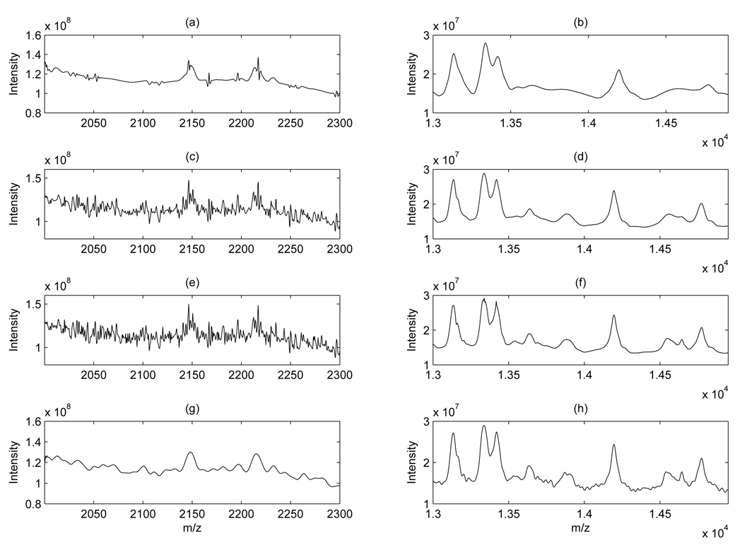
Figure 3 shows a comparison between global wavelet thresholding, with three different threshold values, and our local wavelet thresholding, all applied to the same spectrum shown in Figure 1. Plots in the left column show the 2,000 – 2,300 m/z range and plots in the right column the 13,000 – 15,000 m/z range. Plots (a) and (b) refer to denoising with global wavelet thresholding and threshold given by 30 × σ̂ with σ̂ computed as in (2). Plots (c),(d) and (e),(f) show the same thresholding with a threshold of 10 × σ̂ and 6 × σ̂, respectively. This is the recommended range for C suggested by Coombes et al. [4] for SELDI data. In plots (c) and (e) most of the noise in the lower m/z region has not been removed, while in plots plot (b) and (d) peaks have been reduced in intensity. For comparison, plots (g) and (h) show the same portion of the spectrum denoised with our local thresholding scheme and threshold computed as in (5). The procedure clearly achieves a better removal of the noise while preserving the peaks.

Figure 3.

Ovarian cancer data: Sample spectrum denoised with global thresholding and three different thresholds (30×σ̂, 10×σ̂, and 6×σ̂), plots (a) – (f), and with our local thresholding, plots (g)(h). Left column shows the 2,000 – 2,300 m/z range, right column the 13,000 – 15,000 m/z range.

3.3 Peak Detection

We applied the local thresholding procedure to each of the 50 raw mass spectra. For each spectrum, the variance change point detection method detected a number of change points ranging from 3 to 26. The average number of variance changes was 8. We then applied the local wavelet thresholding to each raw mass spectrum based on the identified segments. We obtained best performances by using thresholds computed as in (5). Using PROcess package in Bioconductor we subtracted the baseline from the denoised mass spectra by fitting a monotone local minimum curve to the data. We finally applied a peak detection procedure to the baseline-subtracted spectra. Peak detection is a crucial step in the identification and quantification of proteins in mass spectra. It is to be expected that a more careful preprocessing of the spectra would result in improved performances of peak detection methods.

We used the peak detection method implemented in the SpecAlign software of Wong et al. [19] and available at physchem.ox.ac.uk/~jwong/specalign. This method has three user-defined inputs: baseline cutoff value, window size, and height ratio. The baseline cutoff value is the fraction of baseline under the cutoff that should be ignored for peak detection. We used the cutoff value 2. The method finds local maxima within a window. We chose a default window size of 31. The height ratio is the ratio between the intensity of a peak maximum and its minimum, i.e., the base of the peak and it is a measure of the signal-to-noise ratio (SNR). We used the value 2. Smaller window sizes and/or height ratios would result in more detected peaks. Our setting is somewhat more conservative that the default setting in SpecAlign.

Following the approach suggested by Morris et al. [20], we looked at peaks detection based on the mean spectrum. In addition, we removed peaks with less than 9,000,000 actual ion count. This value corresponds to an intensity value of 1, which is the recommended threshold in peak detection in order to reduce the inclusion of noisy peaks.

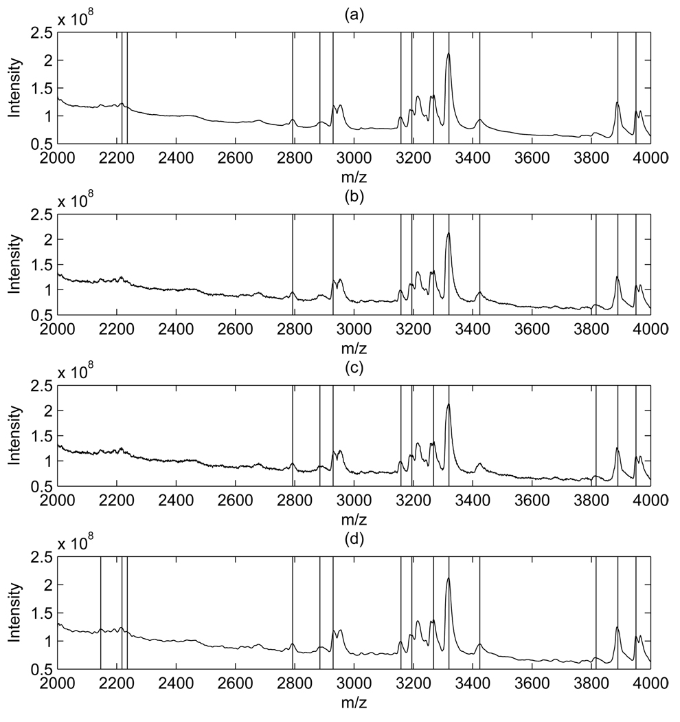
When applied to spectra denoised with our local thresholding, the peak detection method detected 59 peaks over the entire m/z range. When spectra were denoised with the global thresholding of Coombes et al. [4], and C = 30, 10, 6, instead, the detection method identified 48, 51 and 53 peaks, respectively. Figure 4 shows the detected peaks, on the mean spectra, for the low range of m/z values from 2,000 to 4,000. In Figure 4, plots (a), (b) and (c) show results obtained on spectra smoothed with the approach of Coombes et al. [4] and the three chosen thresholds, while plot (d) refers to our approach. The vertical bars indicate the detected peaks. There are 12, 10, 10 and 14 detected peaks in plots (a), (b), (c), and (d) respectively. As expected, our thresholding procedure, which takes into account the heterogeneity of the noise, leads to improved detection performances in the lower m/z part of the spectrum, where the noise has a larger variance. Between 10,000 and 15,000 m/z range we detected 8 peaks, while when using the Coombes et al. approach we found 5, 7, and 7 peaks from different C values, respectively. In Figure 4 three noticeable peaks were missed by both Coombes et al. method and our method. This is due to the relatively conservative setting we chose for SpecAlign.

Figure 4.

Ovarian cancer data: Comparison of global (plots (a), (b), and (d)) and local (plot (d)) thresholding schemes. Vertical lines represent the locations of the detected peaks.

Results here presented did not show much sensitivity to the choice of the wavelet family. Wavelets with higher numbers of vanishing moments are more regular and lead to smoother approximations. On the other hand the support of the wavelets increases with the regularity and boundary effects may arise in the DWT, so that a trade-off is often necessary. We reanalyze the data with our method using Haar wavelets, Daubechies with 3 and 4 vanishing moments, and least asymmetric wavelets with 8 vanishing moments. Except for Haar wavelets all families show very similar denoising and detection performances (results not shown). Haar wavelets resulted in the detection of 55 peaks.

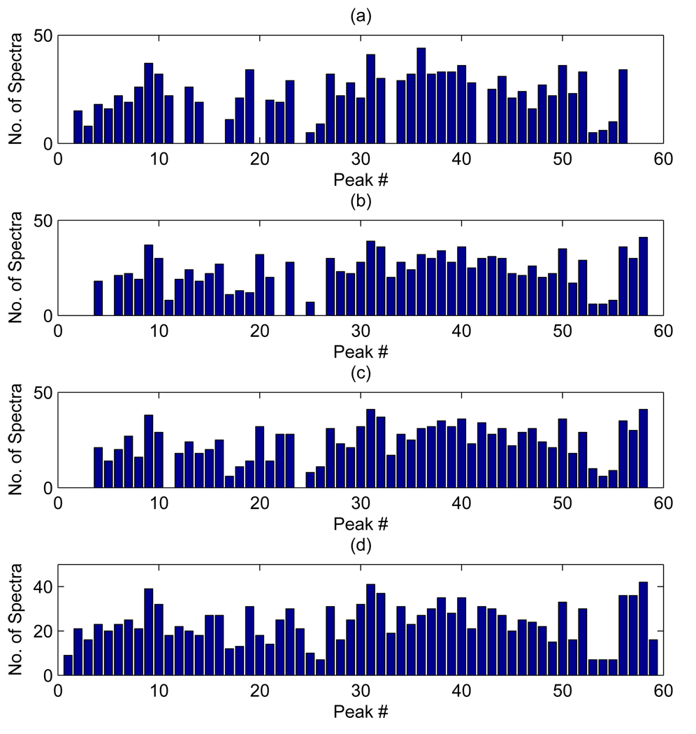
To assess an effect of our denoising procedure on the reproducibility of peak detection algorithms we computed frequencies of detection of single peaks in individual spectra. Mass spectra exhibit shifts along the horizontal axis between replicate spectra. The instruments typically have an accuracy of 0.1 to 0.3% on the m/z scale. Thus, detected peaks that have masses within the percentage accuracy are considered identical. When counting frequencies of detection on the aligned spectra we therefore considered identical peaks that had m/z measurements within 0.2% of each other. For each of the 59 peaks identified by our method Figure 5 reports histograms showing the number of spectra on which the peak is detected. As in the previous figures, plots (a), (b) and (c) refer to results obtained on spectra smoothed with the approach of Coombes et al. [4] and three different thresholds (30 × σ̂, 10 × σ̂, and 6 × σ̂, respectively), while plot (d) refers to our approach. The 59 peaks on the x-axis are ordered according to their m/z value. In general, we notice higher frequencies in plot (d) for almost all peaks, and in particular for those in the lower m/z range.

Figure 5.

Ovarian cancer data: Comparison of global, plots (a), (b), and (c), and local, plot (d), thresholding schemes. Histograms show the number of peaks found in multiple spectra.

3.4 Simulation study

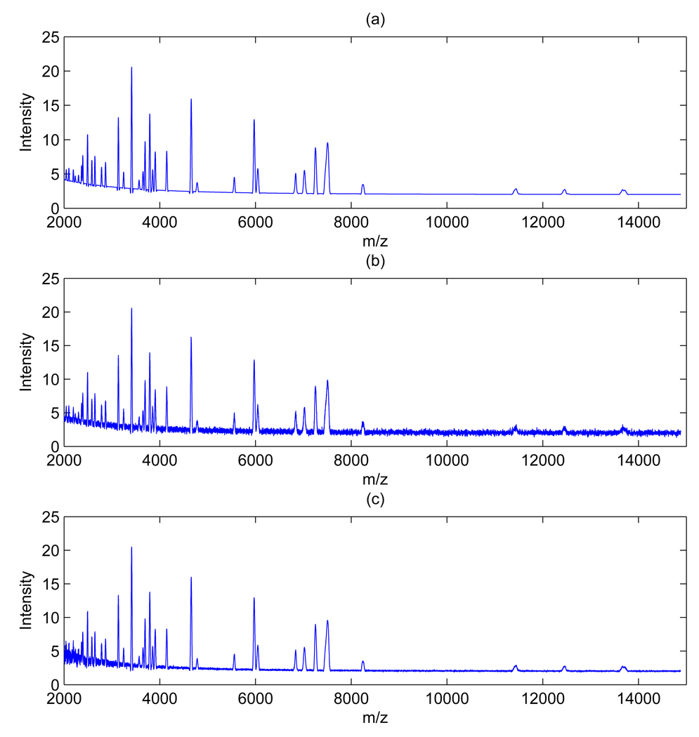
We conclude the paper with a small simulation study to investigate the performances of our local wavelet thresholding procedure. We consider two different scenarios, one where the noise variance is constant, and one where the variance decreases monotonically with the m/z value. The second scenario resembles the ovarian cancer MS spectra analysed in the previous section. We used the SPlus software of Coombes et al. [21] to simulate 50 MS spectra spread over the m/z range from 2,000 to 15,000Da. We considered 50 peaks. The number of peaks in a spectrum varied from 23 to 38. On average a spectrum had 31 peaks. Figure 6 shows one of 50 simulated spectra. The top plot displays a simulated spectrum with baseline, the middle plot shows the spectrum with additive noise and constant variance, and the bottom plot represents the spectrum with additive noise and heteroscedastic variance.

Figure 6.

Simulated MS data: (a) true spectrum, (b) spectrum with additive noise with constant variance, and (c) spectrum with additive noise with a monotonic decreasing variance.

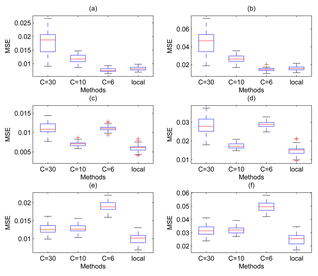
Performances after denoising were computed in terms of mean squared error (MSE)

$${\text{MSE}}_i=\frac{1}{M}{\displaystyle \sum _{j=1}^M{({\widehat{f}}_j^i-f_j^i)}^2,i=1,\dots ,50,}$$

where f̂ⁱ and fⁱ are the i-th denoised and true spectrum, respectively, and M is the number of data points in the i-th spectrum. Figure 7 shows mean squared errors (MSEs) for two thresholding approaches, a global thresholding with threshold λ = 30 × σ̂, 10 × σ̂, and 6 × σ̂ and our local threshold approach with thresholds of type (4). Results are given for the hard thresholding rule, which showed the best performance. The plots in the upper row, (a) and (b), are for constant variance scenario and the plots in the middle row, (c) and (d), for monotonic decreasing variance. Plots (a) and (c) show MSE’s over the whole m/z range, and (b) and (d) for the 2,000 – 5,000 m/z range. In the constant variance setting the two methods gave quite similar results (with C = 6). In the monotonic decreasing variance setting our local wavelet thresholding method performed better than the global method. In addition, since the analysis of real data has suggested possibly correlated errors, we also repeated the simulation study by using autoregressive errors and monotonic decreasing variance. Results are shown in plots (e) and (f) of Figure 7 and have been obtained using the level-dependent thresholds proposed by Johnstone and Silverman for correlated errors. Again, our method shows quite good performances.

Figure 7.

Simulated MS data: Comparison of global and local thresholding schemes over the 2,000 – 15,000 m/z range ((a), (c) and (e)) and the 2,000 – 5,000 m/z range ((b), (d) and (f)). In each plot, the first three boxplots refer to Coombes et al. method with C = 30, C = 10, and C = 6, respectively, and the last boxplot refers to our method. Plots in the upper row, (a) and (b), are for the case of a white noise error with constant variance, plots in the middle row, (c) and (d), for the case of a white noise error and monotonic decreasing variance. Plots in the bottom row, (e) and (f), refer to the case of an autoregressive error with monotonic decreasing variance. Results have been obtained using universal thresholds for the white noise error cases and the level-dependent threshold of Johnstone and Silverman for the case of correlated errors.

In order to assess the effect of the denoising procedure on peak detection performances, we first removed the baseline by using the algorithm implemented in SpecAlign with window size 10. Then we selected peaks from the mean baseline-corrected spectrum. We counted the number of falsely declared peaks and missed true peaks. We report here results for the case of white noise errors. In the constant variance scenario, all methods missed 2 true peaks (one of them under 6,000 m/z) with no false positives. In the monotonic decreasing variance scenario, our method missed 2 peaks (one under 6,000 m/z), while the method of Coombes et al. missed 2, 5, 4 peaks with C = 30, C = 10 and C = 6, respectively. We found no falsely declared peaks for either methods in the two scenarios.

4 Discussion

In mass spectrometry data, intensities in the low m/z range are typically associated to noise with a larger variance than intensities in the higher m/z range. Here we have proposed a wavelet denoising procedure that accounts for the heterogeneous nature of the error term by incorporating a variance change point detection algorithm. Our method is data adaptive and gives better denoising performance. We have shown in simulation and on real data that our denosing procedure leads to improved performances of peaks detection algorithms. In particular, it results in a higher number of detected peaks in the low m/z range and in a higher reproducibility of the results. Both Gaussian white noise and correlated errors have been investigated. In the simulation study we have assumed monotonic decreasing error variance. This assumption, however, is not critical and was used only to obtain simulated data that would resemble the real data analysed in this paper. Another approach, a rescale scheme with global thresholding (similar to Malyarenko, et al. [22]), would be computationally more efficient than our procedure. When the noise variance in the MS data is monotonically decreasing, the rescaling produces a nearly constant variance across the spectrum, and it performs similarly to our procedure for C = 6, while it had inferior performance for C = 30 and C = 10 (data not shown) . However, for any other pattern of variance heterogeneity our method resulted in improved performance, as measured by the MSE, for all choices of C in the global thresholding.

When applying the variance change test we have employed a binary segmentation procedure in order to use the test in a sequential manner. Although different from a simultaneous multiple tests setting, this procedure may result in an inflation of the overall α. In particular, due to the sequential nature of the variance change detection, the overall significance level of each individual change point may be substantially larger than the originally chosen α [23]. However, when applying our local denoising procedure, a falsely detected variance change point implies that there will be two consecutive segments with approximately the same threshold value. While this increases the computational cost of the procedure, it does not affect its performance.

Data file containing the unprocessed raw spectra used in this paper and the Matlab codes to recreate the results can be obtained from our web site at the address http://dceg.cancer.gov/reb.

Abbreviations

DWT

discrete wavelet transform

DWPT

discrete wavelet packet transform

MODWT

maximal overlap discrete wavelet transform

ICSS

iterated cumulative sums of squares

MAD

median absolute deviation

MSE

mean squared error

APPENDIX

A Variance Change Point Detection

We now summarize the variance change point detection algorithm. The procedure is based on the iterated cumulative sums of squares (ICSS) algorithm of Inclán and Tiao [15] that aims at testing and identifying variance changes in a sequence of independent observations from uncorrelated random variables {x_t} with mean 0 and variances ${\sigma }_t^2,t=1,\dots ,T$. Null and alternative hypotheses are specified as

$$H_0:{\sigma }_1^2={\sigma }_2^2=\dots ={\sigma }_T^2\text{ versus }{H}_a:{\sigma }_1^2=\cdots ={\sigma }_k^2\ne {\sigma }_{k+1}^2=\cdots ={\sigma }_T^2.$$

We denote with $C_k={\displaystyle {\sum }_{t=1}^k{x}_t^2}$ the cumulative sum of squares. The test statistic is defined as D = max(D⁺,D⁻) where

$$\begin{array}{c}{D}^{+}=\underset{1\le k\le T-1}{\text{max}}\left(\frac{k+1}{T}-P_k\right),\hfill \\ D^{-}=\underset{1\le k\le T-1}{\text{max}}\left(P_k-\frac{k}{T}\right),\hfill \\ P_k=\frac{C_k}{C_T},k=1,\dots ,T.\hfill \end{array}$$

When the maximum absolute value of D exceeds a certain predetermined value, then we estimate a change at point k* = argmax_kD. Inclán and Tiao [15] showed that when the random variables {x_t} are independent, the asymptotic distribution of D is that one of a Brownian bridge. Whitcher et al. [16] adapted the ICSS algorithm to coefficients from discrete wavelet transforms of long memory data, for which the assumption of uncorrelated data is still reasonable. They suggested to use at least T = 128 sample size to conform with the asymptotic distribution of D. They also obtained predetermined values for D under the null hypothesis by using Monte Carlo simulation. Gabbanini et al. [8] extended the ICSS procedure to discrete wavelet packet transforms (DWPT) and maximal overlap discrete wavelet packet transforms (MODWPT). This allowed them to analyze a broader class of data than just long memory.

A.1 The Binary Segmentation Procedure

The method described above, originally designed for the location of single change points, can be extended to multiple change points via the binary segmentation procedure [15]. At the first stage of the procedure we test the null hypothesis for the whole data. If we do not reject H₀ we declare that there is no change point in the whole sequence, otherwise we divide the data into two sub-sequences as determined by the change point located. At the second stage we test the two sub-sequences and repeat the above procedure until we do not find any further change point. Several candidate change points may result from this procedure. At the third stage we check these points as follows. For a given possible change point we determine the sub-sequence between the previous possible change point and the next change point and repeat the test. If we still reject H₀ we keep this point as a change point, otherwise we remove it from the list of candidates. This confirmatory step helps to reduce masking effect and to get more reliable change point estimates.

In order to take into account the sequential testing of variance change points in the choice of the α-level, we recommend to use a result by Chong (Theorem 3, [23]). Under the null hypothesis of no change point, and with m denoting the number of change points, Chong showed that P_H0(m=0) (m̂ = k) = Φ₀(k)α^k(1 − α)^k+1 for a known constant Φ₀(k) and for a fixed level α that is the same for each test. We therefore choose α such that

$${\displaystyle \sum _{k=1}^M{P}_{H_0}(\widehat{m}=k)={\displaystyle \sum _{k=1}^M{\mathrm{\Phi }}_0(k){\alpha }^k{(1-\alpha )}^{k+1}\le 0.05,}}$$

where M is the upper bound of the number of change points and ${\mathrm{\Phi }}_0(k)=\frac{1}{2k+1}{C}_k^{2k+1}$ with $C_r^n=\frac{n!}{r!(n-r)!}$. We used M = 50.

A.2 Algorithm

The variance change point detection procedure we adopt works as follows.

• Step I: Apply the DWPT and MODWPT. The maximum level of the transforms depends on the length of the data. It is advisable to work with no less than 128 data points when implementing the variance change test.

• Step II: Choose a wavelet packet. The ICSS test for variance changes requires uncorrelated data. As suggested by Gabbanini et al. [8], we use the Ljung-Box test [24] for autocorrelation and select the DWPT packet with highest P-value among those for which the null hypothesis of the test is not rejected. The statistic for this test is defined as

  $$Q=n(n+2){\displaystyle \sum _{k=1}^l\frac{{\widehat{\rho }}^2(k)}{n-k},}$$

  where ρ̂²(k) is a squared correlation coefficient at lag k, l is arbitrary chosen, and n is the length of data. Here we use a lag of 10.

• Step III: Apply the ICSS algorithm. We test for variance changes with the ICSS algorithm using the coefficients of the DWPT packet selected from Step II. If the null hypothesis that no variance change occurs is rejected then we identify the location of the change point using the non-decimated wavelet packet coefficients of the same packet.

• Step IV: Test for multiple changes: Using the binary segmentation procedure we repeat Steps I–III with subsequent subseries until no further variance change point is found. We also perform the additional confirmatory step on all identified potential change points by using subseries of data between adjacent points, as suggested by Inclán and Tiao [15].

References

- 1.Hilario M, Kalousis A, Pellegrini C, Müller M. Processing and classification of protein mass spectra. Mass Spectrometry Reviews. 2006;25:409–449. doi: 10.1002/mas.20072. [DOI] [PubMed] [Google Scholar]
- 2.Shin H, Mutlu M, Koomen JM, Markey MK. Parametric power spectral density analysis of noise from instrumentation in MALDI TOF mass spectrometry. Cancer Informatics. 2006;3:317–328. [PMC free article] [PubMed] [Google Scholar]
- 3.Krutchinsky AN, Chait BT. On the nature of the chemical noise in MALDI mass spectra. Journal of the American Society of Mass Spectrometry. 2002;13:129–134. doi: 10.1016/s1044-0305(01)00336-1. [DOI] [PubMed] [Google Scholar]
- 4.Coombes KR, Tsavachidis S, Morris JS, Baggerly KA, Hung M, Kuerer HM. Improved peak detection and quantification of mass spectrometry data acquired from surface-enhanced laser desorption and ionization by denoising spectra with the undecimated discrete wavelet transform. Proteomics. 2005;5:4107–4117. doi: 10.1002/pmic.200401261. [DOI] [PubMed] [Google Scholar]
- 5.Qu Y, Adam B-L, Thornquist M, Potter JD, Thompson ML, Yasui Y, Davis J, Schellhammer PF, Cazares L, Clements MA. Data reduction using a discrete wavelet transform in discriminant analysis of very high dimensionality data. Biometrics. 2003;59:143–151. doi: 10.1111/1541-0420.00017. [DOI] [PubMed] [Google Scholar]
- 6.Randolph TW, Yasui Y. Multiscale processing of mass spectrometry data. Biometrics. 2006;62:589–597. doi: 10.1111/j.1541-0420.2005.00504.x. [DOI] [PubMed] [Google Scholar]
- 7.Chen S, Hong D, Shyr Y. Wavelet-based procedures for proteomic mass spectrometry data processing. Computational Statistics and Data Analysis. 2007;52:211–220. [Google Scholar]
- 8.Gabbanini F, Vannucci M, Bartoli G, Moro A. Wavelet packet methods for the analysis of variance of time-series with application to crack widths on the Brunelleschi dome. Journal of Computational and Graphical Statistics. 2004;13:639–658. [Google Scholar]
- 9.Donoho DL, Johnstone IM. Ideal spatial adaption by wavelet shrinkage. Biometrika. 1994;81:425–455. [Google Scholar]
- 10.Donoho DL, Johnstone IM. Adapting to unknown smoothness via wavelet shrinkage. Journal of the American Statistical Association. 1995;90:1200–1224. [Google Scholar]
- 11.Mallat SG. A theory of multiresolution signal decomposition: the wavelet representation. IEEE Transactions on Pattern Analysis and Machine Intelligence. 1989;11:674–693. [Google Scholar]
- 12.Percival DB, Walden AT. Wavelet Methods for Time Series Analysis. Cambridge, UK: Cambridge University Press; 2000. [Google Scholar]
- 13.Kwon DW, Tadesse MG, Sha N, Pfeiffer RM, Vannucci M. Identifying biomarkers from mass spectrometry data with ordinal outcome. Cancer Informatics. 2007;3:19–28. [PMC free article] [PubMed] [Google Scholar]
- 14.Johnstone IM, Silverman BW. Wavelet threshold estimators for data with correlated noise. Journal of the Royal Statistical Society, Series B. 1997;59:319–351. [Google Scholar]
- 15.Incláln C, Tiao GC. Use of cumulative sums of squares for retrospective detection of changes of variance. Journal of the American Statistical Association. 1994;89:913–923. [Google Scholar]
- 16.Whitcher B, Guttorp P, Percival DB. Multiscale detection and location of multiple variance changes in the presence of long memory. Journal of Statistical Computation and Simulation. 2000;68:65–88. [Google Scholar]
- 17.DiMagno EP, Corle D, O’Brien JF, Masnyk IJ, Go VLW, Aamodt R. Effect of long-term freezer storage, thawing, and refreezing on selected constituents of serum. Mayo Clin Proc. 1989;64:1226–1234. doi: 10.1016/s0025-6196(12)61285-3. [DOI] [PubMed] [Google Scholar]
- 18.Moore LE, Fung ET, McGuire M, Rabkin CC, Molinaro A, Wang Z, Zhang F, Wang J, Yip C, Meng XY, Pfeiffer RM. Evaluation of apolipoprotein a1 and post-translationally modified forms of transthyretin as biomarkers for ovarian cancer detection in an independent study population. Cancer Epidemiology Biomarkers & Prevention. 2006;15:1641–1646. doi: 10.1158/1055-9965.EPI-05-0980. [DOI] [PubMed] [Google Scholar]
- 19.Wong JW, Cagney G, Cartwright HM. Specalign–processing and alignment of mass spectra datasets. Bioinformatics. 2005;21(9):2088–2090. doi: 10.1093/bioinformatics/bti300. [DOI] [PubMed] [Google Scholar]
- 20.Morris JS, Coombes KS, Kooman J, Baggerly KA, Kobayashi R. Feature extraction and quantification for mass spectrometry data in biomedical applications using the mean spectrum. Bioinformatics. 2005;21(9):1764–1775. doi: 10.1093/bioinformatics/bti254. [DOI] [PubMed] [Google Scholar]
- 21.Coombes KR, Koomen JM, Baggerly KA, Morris JS, Kobayashi R. Understanding the characteristics of mass spectrometry data through the use of simulation. Cancer Informatics. 2005;1:41–52. [PMC free article] [PubMed] [Google Scholar]
- 22.Malyarenko DI, Cooke WE, Adam B-L, Malik G, Chen H, Tracy ER, Trosset MW, Sasinowski M, Semmes OJ, Manos DM. Enhancement of sensitivity and resolution of surface-enhanced laser desorption/ionization time-of-flight mass spectrometric records for serum peptides using time-series analysis techniques. Clinical Chemistry. 2005;51:65–74. doi: 10.1373/clinchem.2004.037283. [DOI] [PMC free article] [PubMed] [Google Scholar]
- 23.Chong TTL. Estimating the locations and number of change points by the sample-splitting method. Statistical papers. 2001;42(1):53–79. [Google Scholar]
- 24.Ljung GM, Box GEP. On a measure of lack of fit in time series models. Biometrika. 1978;65:297–304. [Google Scholar]