Multivariate Tensor-based Morphometry on Surfaces: Application to Mapping Ventricular Abnormalities in HIV/AIDS

Abstract

Here we developed a new method, called multivariate tensor-based surface morphometry (TBM), and applied it to study lateral ventricular surface differences associated with HIV/AIDS. Using concepts from differential geometry and the theory of differential forms, we created mathematical structures known as holomorphic one-forms, to obtain an efficient and accurate conformal parameterization of the lateral ventricular surfaces in the brain. The new meshing approach also provides a natural way to register anatomical surfaces across subjects, and improves on prior methods as it handles surfaces that branch and join at complex 3D junctions. To analyze anatomical differences, we computed new statistics from the Riemannian surface metrics - these retain multivariate information on local surface geometry. We applied this framework to analyze lateral ventricular surface morphometry in 3D MRI data from 11 subjects with HIV/AIDS and 8 healthy controls. Our method detected a 3D profile of surface abnormalities even in this small sample. Multivariate statistics on the local tensors gave better effect sizes for detecting group differences, relative to other TBM-based methods including analysis of the Jacobian determinant, the largest and smallest eigenvalues of the surface metric, and the pair of eigenvalues of the Jacobian matrix. The resulting analysis pipeline may improve the power of surface-based morphometry studies of the brain.

1. Introduction

Surface-based analysis methods have been extensively used to study structural features of the brain, such as cortical gray matter thickness, complexity, and patterns of brain change over time due to disease or developmental processes (Thompson and Toga, 1996; Dale et al., 1999; Thompson et al., 2003; Chung et al., 2005). Cortical mapping methods have revealed the 3D profile of structural brain abnormalities in Alzheimer’s disease, HIV/AIDS, Williams syndrome, epilepsy, schizophrenia, and bipolar disorder (Thompson et al., 2003, 2004b, 2005a,b, 2009). Surface models have also proven useful for studying the shape of subcortical structures such as the hippocampus, basal ganglia, and ventricles (Thompson et al., 2004a; Styner et al., 2004, 2005; Yushkevich et al., 2006; Morra et al., 2009).

One fruitful area of research combines surface-based modeling with deformation-based methods that measure systematic differences in structure volumes and shapes. Deformation-based morphometry (DBM) (Ashburner et al., 1998; Chung et al., 2001; Wang et al., 2003; Chung et al., 2003b), for example, uses deformations obtained from the nonlinear registration of brain images to a common anatomical template, to infer 3D patterns of statistical differences in brain volume or shape. Tensor-based morphometry (TBM) (Davatzikos et al., 1996; Thompson et al., 2000a; Chung et al., 2003a; Ashburner, 2007; Leporé et al., 2008; Chung et al., 2008) is a related method, that examines spatial derivatives of the deformation maps that register brains to common template. Morphological tensor maps are used to derive local measures of shape characteristics such as the Jacobian determinant, torsion or vorticity. DBM, by contrast, analyzes 3D displacement vector fields encoding relative positional differences in anatomical structures across subjects, after mapping all brain images to a common stereotaxic space (Thompson et al., 1997; Cao et al., 1997). One advantage of TBM for studying brain structure is that it also derives local derivatives and tensors from the deformation for further analysis. When applied to surface models, TBM can even make use of the Riemannian surface metric to characterize local surface abnormalities. In this paper, we extend tensor-based morphometry to the multivariate analysis of surface tensors. We illustrate the approach by applying it to analyze lateral ventricular surface abnormalities in patients with HIV/AIDS. The overall goal of the work is to find new and informative descriptors of local shape differences that can pick up disease effects with greater statistical power than standard methods.

The lateral ventricles – fluid-filled structures deep in the brain – are often enlarged in disease, and can provide sensitive measures of disease progression. Surface-based analysis approaches have been applied in many studies to examine ventricular surface morphometry (Thompson et al., 2004a; Styner et al., 2005; Thompson et al., 2006; Carmichael et al., 2006; Ferrarini et al., 2006; Carmichael et al., 2007a,b,c; Ferrarini et al., 2008a,b; Chou et al., 2008, 2009a,b). Ventricular changes typically reflect atrophy in surrounding structures, and ventricular measures and surface-based maps often provide sensitive (albeit indirect) assessments of tissue reduction that correlate with cognitive deterioration in illnesses. Ventricular measures have also recently garnered interest as good biomarkers of progressive brain change in dementia. They can usually be extracted from brain MRI scans with greater precision than hippocampal surfaces or other models (Weiner, 2008).

Thompson et al. (2004a, 2006) analyzed ventricular shape with a parametric surface-based anatomical modeling approach originally proposed in (Thompson and Toga, 1996). In one type of analysis, a medial axis is derived passing down the center of each ventricular horn. The local radial size – an intuitive local measure of thickness – can then be defined as the radial distance between each boundary point and its closest point on the associated medial axis (see Thompson et al. (2004a) for details; see work by Styner and Yushkevich for related ‘m-rep’ approaches). Based on the local radial size, multiple regression, or structural equation models (Chou et al., 2009b), may be used to assess the simultaneous effects of multiple factors or covariates of interest, on surface morphology. Given maps of surface-based statistics, false discovery rate (FDR) methods or permutation methods may be used to assign overall (corrected) p-values for effects seen in surface based statistical maps. In the largest ventricular mapping study to date (N = 339), Carmichael et al. (2006) applied the radial distance method together with an automated single-atlas segmentation method to analyze localized ventricular expansion in Alzheimer’s disease (AD) and mild cognitive impairment. This method was also applied in a series of ventricular expansion studies (Carmichael et al., 2007a,b,c). More recently, the same method was also extended to combine multiple segmentations (using an approach called “multi-atlas fluid image alignment”) to create more accurate segmentations of the ventricular surface. These methods have been used to study genetic effects in AD (Chou et al., 2008), genetic influences on ventricular structure in normal adult twins (Chou et al., 2009b). These methods found correlations between ventricular expansion and CSF biomarkers of pathology, and with baseline and future clinical decline (Chou et al., 2009a).

Styner et al. (2005) also modeled the lateral ventricles using geometrical surfaces, by transforming each ventricle into a spherical harmonic-based shape description. They applied this method to explore the effects of heritability and genetic risk for schizophrenia on ventricular volume and shape. Extending this work to a diagnostic classification problem, Ferrarini et al. (2007) used an unsupervised clustering algorithm, generating a control average surface and a cloud of corresponding nodes across a dataset, to study ventricular shape variations in healthy elderly and AD subjects (Ferrarini et al., 2006, 2008a,b).

As an illustrative application, we studied ventricular surface abnormalities associated with HIV/AIDS. Our proposed multivariate TBM method detected areas of statistically significant deformation even in a relatively small test dataset – from 11 subjects with HIV/AIDS and 8 matched healthy controls². For comparison, we also compared our multivariate TBM method with simpler, more standard, Jacobian matrix based statistics. In a comparison of overall effect sizes for different surface-based statistics, our multivariate TBM method detected areas of abnormality that were generally consistent with simpler approaches, but gave greater effect sizes (and therefore greater statistical power) than all other Jacobian matrix based statistics including the Jacobian determinant, largest and least eigenvalue, or the pair of eigenvalues of the local Jacobian matrix. Our method to compute the Jacobian matrix and multivariate TBM is also quite general and can be used with other surface models and triangulated meshes from other analysis programs used in neuroimaging (Fischl et al., 1999; Van Essen et al., 2001; Thompson et al., 2004b).

Figure 1 summarizes our overall sequence of steps used to analyze lateral ventricular surface morphometry. We used lateral ventricular surface models from our previously published study (Thompson et al., 2006). We deliberately chose a small set of surfaces, to see if group differences were detectable in a small sample, and if so, we aimed to find out which surface-based statistics gave greatest effect sizes for detecting these differences. Constrained harmonic map (Joshi et al., 2007; Shi et al., 2007) was used to match ventricular surfaces and multivariate statistics were applied to identify regions with significant differences between the two groups. Based on this, we created statistical maps of group differences.

Figure 1.

A flow chart shows how canonical holomorphic one-forms are used to model ventricular shape, and how the resulting surfaces are analyzed using multivariate tensor-based morphometry. After ventricular surfaces are extracted from MRI images either manually or automatically (Thompson et al., 2006), surfaces are automatically partitioned into three pieces by computing canonical holomorphic one-forms. For each element of the partitioned surface, we compute a new conformal coordinates and register surfaces with a constrained harmonic map. The statistics of multivariate TBM are computed at each point on the resulting matching surfaces, revealing regions with systematic anatomical differences between groups.

2. Automatic Surface Registration with Holomorphic One Forms

2.1. Theoretical Background

Differential forms are used here as the basis for surface modeling and parameterization. They belong to a branch of differential geometry known as the exterior calculus. Basic principles of these mathematical constructs are reviewed here, assuming some knowledge of differential geometry. For a more detailed introduction to differential forms, the reader is referred to a differential geometry text such as Bachman (2006).

Suppose S is a surface embedded in ℝ³, with induced Euclidean metric g. In the terminology of differential geometry, S is considered to be covered by an atlas {(U_α, φ_α)}. Suppose (x_α, y_α) is the local parameter on the chart (U_α, φ_α). We say that a coordinate system (x_α, y_α) for the surface is isothermal, if the metric has the representation $\mathbf{g}=e^{2\lambda (x_{\alpha },y_{\alpha })}({dx}_{\alpha }^2+{dy}_{\alpha }^2)$, where λ(x_α, y_α) is the conformal factor, which is a positive scalar function defined on each point on the surface.

The Laplace-Beltrami operator is defined as

$${\mathrm{\Delta }}_{\mathbf{g}}=\frac{1}{e^{2\lambda (x_{\alpha },y_{\alpha })}}(\frac{{\partial }^2}{\partial x_{\alpha }^2}+\frac{{\partial }^2}{\partial y_{\alpha }^2}).$$

This operator may be used to measure the regularity (smoothness) of signals that are defined on a surface, and it is the extension of the standard Laplacian operator to general manifolds, such as curved surfaces. A function f: S → ℝ is harmonic, if Δ_gf ≡ 0.

Suppose ω is a differential one-form with the representation f_αdx_α+g_αdy_α in the local parameters (x_α, y_α), and f_βdx_β + g_βdy_β in the local parameters (x_β, y_β). Then

$$\left(\begin{array}{cc}\frac{\partial x_{\alpha }}{\partial x_{\beta }}& \frac{\partial y_{\alpha }}{\partial x_{\beta }}\\ \frac{\partial x_{\alpha }}{\partial y_{\beta }}& \frac{\partial y_{\alpha }}{\partial y_{\beta }}\end{array}\right)\left(\begin{array}{c}{f}_{\alpha }\\ g_{\alpha }\end{array}\right)=\left(\begin{array}{c}{f}_{\beta }\\ g_{\beta }\end{array}\right).$$

ω is a closed one-form, if on each chart (x_α, y_α), $\frac{\partial f}{\partial y_{\alpha }}-\frac{\partial g}{\partial x_{\alpha }}=0$. ω is an exact one-form, if it equals the gradient of some function. An exact one-form is also a closed one-form. The de Rham cohomology group H¹(S, ℝ) is the quotient group between closed one-forms and exact one-forms. If a closed one-form ω satisfies $\frac{\partial f}{\partial x_{\alpha }}+\frac{\partial g}{\partial y_{\alpha }}=0$, then ω is a harmonic one-form. Hodge theory claims that in each cohomology class, there exists a unique harmonic one-form. The gradient of a harmonic function is an exact harmonic one-form.

The Hodge star operator turns a one-form ω into its conjugate ^*ω, ^*ω = −g_αdx_α + f_αdy_α. If we rewrite the isothermal coordinates (x_α, y_α) in the complex format z_α = x_α + iy_α, then the isothermal coordinate charts form a conformal structure on the surface. A topological surface with a conformal structure is called a Riemann surface.

Holomorphic differential forms may be generalized to Riemann surfaces by using the notion of conformal structure. A holomorphic one-form is a complex differential form, such that on each chart, it has the form $f(z)dz=\omega +\sqrt{-1}{}^{\ast }\omega$, where ω is a harmonic one-form, and f(z) is a holomorphic function. All holomorphic one-forms form a linear space, which is isomorphic to the first cohomology group H¹(S, ℝ).

For a genus 0 open boundary surface with s boundaries, all holomorphic one-forms form a real s-dimensional linear space. At a zero point p ∈ M of a holomorphic one-form ω, any local parametric representation has

$$\omega =f(z_{\alpha })d{z}_{\alpha },f{\mid }_p=0.$$

In general there are s − 1 zero points for a holomorphic one-form defined on a genus 0 open boundary surface with s boundaries.

A holomorphic one-form induces a special system of curves on a surface, the so-called conformal net. Horizontal trajectories are the curves that are mapped to iso-v lines in the parameter domain. Similarly, vertical trajectories are the curves that are mapped to iso-u lines in the parameter domain. The horizontal and vertical trajectories form a web on the surface. The trajectories that connect zero points, or a zero point with the boundary, are called critical trajectories. The critical horizontal trajectories form a graph, called the critical graph.

2.2. Illustration in the 2D Planar Case

Suppose we have an analytic function φ: z → w, z, w ∈ ℂ, that maps the complex z-plane to the complex w-plane. We will demonstrate the concepts of the holomorphic one-form, a conformal net, and our proposed algorithms, by using three simple planar cases.

For simplicity, we simply choose φ as the function that squares a complex number, i.e., w = z²; the mapping caused by this function may be considered to be a deformed grid in the complex plane, which is visualized in Figure 2(a) and (b). The holomorphic one-form is the complex differential dw = 2zdz. The red and blue curves in the w-plane are the horizontal trajectories and vertical trajectories of dw. They are mapped to the red and blue lines in the w-plane. The conformal net is formed by horizontal and vertical trajectories. We examine a horizontal trajectory γ; φ maps γ to a horizontal line, namely, along γ the imaginary part of the differential form dw is always zero. Similarly, along a vertical trajectory, the real part of dw is always zero.

Figure 2.

Illustration of conformal net on various surfaces. (a) is w-plane, where w = z²; (b) is the z-plane. (c) and (d) illustrate the conformal nets on genus 0 surfaces with 2 and 4 open boundaries, respectively. Horizontal trajectories (blue) and vertical trajectories (red) are illustrated in (b)–(d). (c) is topologically equivalent to the ventricular surface after the topology change.

Therefore, in order to trace horizontal trajectories, we only need to find a direction, along which the value of the differential form is real. Similarly, the vertical trajectories may be traced by following directions in which dw is always imaginary.

The center of the z-plane is a zero point, which is mapped to the origin of the w-plane. In the neighborhood of the zero point, the horizontal trajectories may be represented as the level sets

$$x^2-y^2=\mathit{const},$$

and the vertical trajectories may be represented, by the implicit function

$$xy=\mathit{const},$$

– both of these are hyperbolic curves.

At the zero point, more than one of the horizontal trajectories intersect with each other, and more than one of the vertical trajectories intersect with each other. The trajectories through the zero point are called critical trajectories. The horizontal critical trajectories partition the z-plane into 4 patches. Each patch is mapped by φ to a half plane in the w-plane.

Suppose z₀ is the zero point on the z-plane, the map φ may be recovered by integrating the differential form, ω, namely

$$w=\phi (z)={\int }_{z_0}^z\omega .$$ (1)

Now, suppose instead that we have an analytic map from a 2-hole annulus (a simple type of surface) to the complex plane. In Figure 2(c), we visualize the map in the same way as in the previous discussion.

We denote the differential form of the map as ω. The horizontal and vertical trajectories in the z-plane are represented as red and blue curves, which are mapped to the horizontal and vertical lines in w-plane.

It is still true that along horizontal trajectories, the imaginary part ω is zero; along vertical trajectories, the real component of ω is zero. The zero point is the intersection of two horizontal trajectories and also of two vertical trajectories. The horizontal and vertical trajectories form the conformal net. Similarly, we illustrate an analytic map from a 4-hole annulus to the complex plane in Figure 2(d). There are three zero points.

The conformal net has a simple global structure. The critical graph partitions the surface into a set of non-overlapping patches that jointly cover the surface, and each patch is either a topological disk or a topological cylinder (Strebel, 1984). This is important because it allows a general surface to be converted into a set of non-overlapping parametric meshes, even if the surface has holes or branches in it. Each patch Ω ⊂ M may be mapped to the complex plane by integration of the holomorphic one-form on it (Equation 1). We will use this property to automatically partition the ventricular surface (Section 4.1). After being cut open at three extreme points, the surface becomes topologically equivalent to a genus 0 with 2 open boundary surface (see Figure 2(c)).

The structure of the critical graph and the parameterizations of the patches are determined by the conformal structure of the surface. If two surfaces are topologically homeomorphic to each other and have similar geometrical structures, they can support consistent critical graphs and segmentations (i.e., surface partitions), and their parameterizations are consistent as well. Therefore, by matching their parameter domains, the entire surfaces can be directly matched in 3D (this could be considered an induced mapping, or a push-forward mapping, in the terminology of differential geometry). This generalizes prior work in medical imaging that has matched surfaces by computing a smooth bijection to a single canonical surface, such as a sphere or disk (Fischl et al., 1999; Thompson et al., 2000b).

2.3. Algorithm to Compute Canonical Holomorphic One-forms

Suppose that the input mesh has n+1 boundaries, ∂M = γ₀–γ₁–···–γ_n. Without loss of generality, we map γ₀ to the outer boundary and the others to the inner boundaries in the parameter domain.

The following is the algorithm pipeline to compute the canonical holomorphic one-forms:

1. Compute the basis for all exact harmonic one-forms;

2. Compute the basis for all harmonic one-forms;

3. Compute the basis for all holomorphic one-forms;

4. Construct the canonical conformal parameterization.

2.3.1. Basis for Exact Harmonic One-forms

The first step of the algorithm is to compute the basis for exact harmonic one-forms. Let γ_k, k = 1, …, n, be an internal boundary, we compute a harmonic function f_k: S → ℝ by solving the following Dirichlet problem on the mesh M:

$$\{\begin{array}{l}\mathrm{\Delta }{f}_k\equiv 0\hfill \\ f_k{\mid }_{{\gamma }_j}={\delta }_{kj}\hfill \end{array}$$

where δ_kj is the Kronecker function, and Δ is the discrete Laplace-Beltrami operator implemented using the co-tangent formula proposed in (Pinkall and Polthier, 1993).

The exact harmonic one-form η_k can be computed as the gradient of the harmonic function f_k, η_k = df_k, and {η₁, η₂, ···, η_n} form the basis for all the exact harmonic one-forms.

2.3.2. Basis for Harmonic One-forms

After getting the exact harmonic one-forms, we will compute the closed one-form basis. Let γ_k (k > 0) be an inner boundary. Compute a path from γ_k to γ₀, denote it by ζ_k. ζ_k cuts the mesh open to M_k, while ζ_k itself is split into two boundary segments ${\zeta }_k^{+}$ and ${\zeta }_k^{-}$ in M_k. Define a function g_k: M_k → ℝ by solving a Dirichlet problem,

$$\{\begin{array}{l}\mathrm{\Delta }{g}_k\equiv 0\hfill \\ g_k{\mid }_{{\zeta }_k^{+}}=1\hfill \\ g_k{\mid }_{{\zeta }_k^{-}}=0.\hfill \end{array}$$

Compute the gradient of g_k and let τ_k = dg_k, then map τ_k back to M, where τ_k becomes a closed one-form. Then we need to find a function h_k: M → ℝ, by solving the following linear system: Δ(τ_k + dh_k) ≡ 0.

Updating τ_k to τ_k + dh_k, we now have {τ₁, τ₂, …, τ_n} as a basis set for all the closed but non-exact harmonic one-forms.

With both the exact harmonic one-form basis and the closed non-exact harmonic one-form basis computed, we can construct the harmonic one-form basis by taking the union of them: {η₁, η₂, ···, η_n; τ₁, τ₂, ···, τ_n}.

2.3.3. Basis for Holomorphic One-forms

In Step 1, we computed the basis for exact harmonic one-forms {η₁, ···, η_n}. Now we compute their conjugate one-forms {^*η₁, ···, ^*η_n}, so that we can combine all of them together into a holomorphic one-form basis set.

First of all, for η_k we compute an initial approximation ${\eta }_k^{\prime }$ by a brute-force method using the Hodge star. That is, rotating η_k by 90° about the surface normal to obtain ${\eta }_k^{\prime }$ (Wang et al., 2007). In practice such an initial approximation is usually not accurate enough because of the digitization errors introduced in the image segmentation and surface reconstruction steps. To improve accuracy, we employ a technique that uses the harmonic one-form basis that we just computed. From the fact that η_k is harmonic, we can conclude that its conjugate ^*η_k should also be harmonic. Therefore, ^*η_k may be represented as a linear combination of the base harmonic one-forms:

$${{}^{\ast }\eta }_k=\sum _{i=1}^n{a}_i{\eta }_i+\sum _{i=1}^n{b}_i{\tau }_i.$$

Using the wedge product ∧ (Heinbockel, 2001), we can construct the following linear system,

$${\int }_M{{}^{\ast }\eta }_k\wedge {\eta }_i={\int }_M{\eta }_k^{\prime }\wedge {\eta }_i,{\int }_M{{}^{\ast }\eta }_k\wedge {\tau }_j={\int }_M{\eta }_k^{\prime }\wedge {\tau }_j.$$

We solve this linear system to obtain the coefficients a_i and b_i (i = 1, 2, ···, n) for the conjugate one-form ^*η_k. Pairing each base exact harmonic one-form in the basis with its conjugate, we get a basis set for the holomorphic one-form group on M:

$$\{{\eta }_1+\sqrt{-1}{{}^{\ast }\eta }_1,\cdots ,{\eta }_n+\sqrt{-1}{{}^{\ast }\eta }_n\}.$$

2.3.4. Canonical Conformal Parameterization

Given a Riemann surface M, there are infinitely many holomorphic one-forms, but each of them may be expressed as a linear combination of the basis elements. Figure 3 illustrates four different holomorphic one-forms on a left lateral ventricular surface. Its induced conformal parameterization is visualized by the texture mapping of a checkerboard onto the surface. We define a canonical conformal parametrization as a linear combination of the holomorphic bases ${\omega }_i={\eta }_i+\sqrt{-1}{{}^{\ast }\eta }_i$, i = 1, …, n. A canonical conformal holomorphic one-form can be computed by

Figure 3.

Illustration of various holomorphic one-forms on a left ventricular surface, generated by using different linear combinations of elements of the holomorphic one-form basis. The holomorphic one-form and its induced conformal parametrization (by Equation 2) are visualized by the texture mapping of a checkerboard onto the surface, such that the checkerboard pattern is uniform in the parameter space. (a) is the canonical conformal parameterization. We use it for surface registration. (b)–(d) show highly irregular areas around the ends of different horns of the ventricles.

$$\omega =\sum _{i=1}^n{\omega }_i.$$ (2)

The conformal parametrization induced by Equation 1 from the canonical conformal holomorphic one-form is called the canonical conformal parametrization, as visualized in Figure 3(a). The selected canonical conformal parameterization has a more uniform parameterization on each horn, which is very useful as it can be used to study the surface morphology of each horn. Compared with our prior work (Wang et al., 2007), the current canonical conformal parameterization directly works on open boundary surfaces and does not require us to compute a double covering of the surface and a homology basis. So, it is more computationally efficient. The obtained conformal parameterization is unique, so it provides a consistent parameterization across surfaces. Another benefit of this specific parameterization is that it maximizes the uniformity of the induced grid over the entire domain, in the sense of optimizing a conformal energy.

2.4. Surface Registration by Constrained Harmonic Map

The canonical conformal parameterization, obtained using this method, is an intrinsic property of the overall surface structure (i.e., depends on its boundary number, and how the components of the surface join in 3D). As a result, the surface partitions that are obtained from modeling different subjects’ anatomy are very similar, and the surface of the ventricles is split up into horns in a logical and consistent way. Thus, we can also match entire surfaces through the parameter domain. There are numerous nonrigid surface registration algorithms (Holden, 2008) that can be applied to register each segmented surface via the parameter domain. To register these surfaces to each other, here we apply a constrained harmonic map through the parameter domain. The constrained harmonic map can be computed as follows.

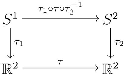
Given two surfaces S₁ and S₂, whose conformal parameterizations are τ₁: S₁ → ℝ² and τ₂: S₂ → ℝ², we want to compute a map, φ: S₁ → S₂. Instead of directly computing φ, we can easily find a harmonic map between the parameter domains. We look for a harmonic map, τ: ℝ² → ℝ², such that

$$\tau \circ {\tau }_1(S_1)={\tau }_2(S_2),\tau \circ {\tau }_1(\partial S_1)={\tau }_2(\partial S_2),\mathrm{\Delta }\tau =0.$$

Then the map φ can be obtained by $\phi ={\tau }_1\circ \tau \circ {\tau }_2^{-1}$. The below diagram illustrates the mapping relationship.

Since τ is a harmonic map, and τ₁ and τ₂ are conformal maps, the resulting φ is a harmonic map. When landmark curves needs to be matched, such as the boundaries of each component of the ventricles, we guarantee the matching of both ends of the curves. We also match the rest of the curves in 3D based on unit speed parameterizations of both curves.

3. Multivariate Tensor-Based Morphometry

3.1. Derivative Map

Suppose φ: S₁ → S₂ is a map from the surface S₁ to the surface S₂. To simplify the formulation, we use the isothermal coordinates of both surfaces as the arguments. Let (u₁, v₁); (u₂, v₂) be the isothermal coordinates of S₁ and S₂, respectively. The Riemannian metric of S_i is represented as ${\mathbf{g}}_i=e^{2{\lambda }_i}(d{u}_i^2+d{v}_i^2)$, i = 1,2.

In the local parameters, the map φ can be represented as φ(u₁, v₁) = (φ₁(u₁, v₁), φ₂(u₁, v₁)). The derivative map of φ is the linear map between the tangent spaces, dφ: TM(p) → TM(φ(p)), induced by the map φ. In the local parameter domain, the derivative map is the Jacobian of φ,

$$d\phi =\left(\begin{array}{cc}\frac{\partial {\phi }_1}{\partial u_1}& \frac{\partial {\phi }_1}{\partial v_1}\\ \frac{\partial {\phi }_2}{\partial u_1}& \frac{\partial {\phi }_2}{\partial v_1}\end{array}\right).$$

Let the position vector of S₁ be r(u₁, v₁). Denote the tangent vector fields as $\frac{\partial }{\partial u_1}=\frac{\partial \mathbf{r}}{\partial u_1},\frac{\partial }{\partial v_1}=\frac{\partial \mathbf{r}}{\partial v_1}$. Because (u₁, v₁) are isothermal coordinates, $\frac{\partial }{\partial u_1}$ and $\frac{\partial }{\partial v_1}$ only differ by a rotation of π/2. Therefore, we can construct an orthonormal frame on the tangent plane on S₁ as { $e^{-{\lambda }_1}\frac{\partial }{\partial u_1},e^{-{\lambda }_1}\frac{\partial }{\partial v_1}$}. Similarly, we can construct an orthonormal frame on S₂ as { $e^{-{\lambda }_2}\frac{\partial }{\partial u_2},e^{-{\lambda }_2}\frac{\partial }{\partial v_2}$}.

The derivative map under the orthonormal frames is represented as

$$d\phi =e^{{\lambda }_2-{\lambda }_1}\left(\begin{array}{cc}\frac{\partial {\phi }_1}{\partial u_1}& \frac{\partial {\phi }_1}{\partial v_1}\\ \frac{\partial {\phi }_2}{\partial u_1}& \frac{\partial {\phi }_2}{\partial v_1}\end{array}\right).$$

In practice, smooth surfaces are approximated by triangle meshes. The map φ is approximated by a simplicial map, which maps vertices to vertices, edges to edges and faces to faces. The derivative map dφ is approximated by the linear map from one face [v₁, v₂, v₃] to another one [w₁, w₂, w₃]. First, we isometrically embed the triangle [v₁, v₂, v₃],[w₁, w₂, w₃] onto the plane ℝ²; the planar coordinates of the vertices of v_i, w_j are denoted using the same symbols v_i, w_j. Then we explicitly compute the linear matrix for the derivative map dφ,

$$d\phi =[w_3-w_1,w_2-w_1]{[v_3-v_1,v_2-v_1]}^{-1}.$$ (3)

3.2. Multivariate Deformation Tensor-Based Statistics

In our work, we use multivariate statistics on deformation tensors (Leporé et al., 2008) and here we adapt these concepts to be applicable to surface tensors. In related work, Chung et al. (2003a, 2008) have also proposed to use the surface metrics as the basis for morphometry in cortical studies. Let J be the derivative map and define the deformation tensors as S = (J^TJ)^1/2. Instead of analyzing shape differences based on the eigenvalues of the deformation tensor, e.g. Cai (2001), we use a recently introduced family of metrics, the “Log-Euclidean metrics” (Arsigny et al., 2006). These metrics make computations on tensors easier to perform, as they are chosen such that the transformed values form a vector space, and statistical parameters can then be computed easily using standard formulae for Euclidean spaces (Wang et al., 2008b).

We apply Hotelling’s T² test (Hotelling, 1931) on sets of values in the Log-Euclidean space of the deformation tensors. Given two groups of n-dimensional vectors S_i, i = 1, …, p, T_j, j = 1, …, q, we use the Mahalanobis distance M to measure the difference between the mean vectors for two different groups of subjects,

$$M=(\mathit{log}\overline{S}-\mathit{log}\overline{T}){\mathrm{\sum }}^{-1}(\mathit{log}\overline{S}-\mathit{log}\overline{T})$$

where S̄ and T̄ are the means of the two groups and Σ is the combined covariance matrix of the two groups. In this formula, the 3 distinct components of the deformation tensor, which is a 2 × 2 symmetric matrix and has two duplicate off-diagonal terms, are converted to a vector of the same dimension.

4. Results

4.1. Automatic Lateral Ventricular Surface Registration via Holomorphic One-Forms

The concave shape, complex branching topology and extreme narrowness of the inferior and posterior horns of the lateral ventricles have made it difficult for surface parameterization approaches to impose a grid on the entire lateral ventricular structure without introducing significant area distortion. For example, many papers in the engineering literature that claim to have extracted the lateral ventricles tend to show the inferior horn omitted or too short; the occipital horn is often also truncated at the calcar avis, but there is usually an additional small volume of CSF at the occipital tip of the occipital horns, and this is hard for most segmentation algorithms to properly connect with the rest of the ventricles. To correctly model the entire lateral ventricular surface, we automatically locate and introduce three cuts on each ventricle. The cuts are motivated by examining the topology of the lateral ventricles, in which several horns are joined together at the ventricular “atrium” or “trigone”. Meanwhile, we keep the cutting curves consistent across surfaces. After the topology is modeled in this way, a lateral ventricular surface, in each hemisphere, becomes an open boundary surface with 3 boundaries(see Figure 4(a)). We computed the exact harmonic one-form (Figure 4(b)), its conjugate one-form (Figure 4(c)), and canonical holomorphic one-form (Figure 4(d). With the conformal net introduced in this way (Figure 4(e)), each lateral ventricular surface may be divided into 3 pieces (Figure 4(f)). Although surface geometry is widely variable across subjects, the zero point locations are intrinsically determined by the surface conformal structures, and the partitioning of the surface into component meshes is highly consistent across subjects. This topological decomposition, to model the structure as a set of connected surfaces, may be considered to be a topology optimization operation. The topological optimization also helps to enable a uniform parametrization on some areas that otherwise are very difficult for usual parametrization methods to capture (e.g., the tips of a pointed structure). Figure 4(f) illustrates the automatic surface segmentation result for the same pair of lateral ventricular surfaces, which is similar to the manual surface segmentations used in prior research (Thompson et al., 2006). Even so, the new automated partitioning method improves on past work as it avoids arbitrarily chopping the surface into 3 parts using a fixed coronal plane. Figure 5 illustrates a pair of segmentation results from two groups. In the Figure, part (a) shows a pair of ventricular surfaces extracted from a 3D MRI image of a healthy control subject and (b) is from a patient with HIV/AIDS. The ventricular surfaces in (b) are dilated due to the disease. The two surfaces are similar overall, so the surface segmentation results are consistent. Each ventricular surface was automatically segmented into 3 pieces. We labeled each piece with a different color. Figure 5 demonstrates that our algorithm can successfully identify matching parts on surfaces that are significantly different.

Figure 4.

Illustration of automatic lateral ventricular surface segmentation via holomorphic one-forms. (a). Topology change. Three cuts were made on each ventricular surface “extreme points”. (b). One computed exact harmonic one-form, which is visualized by integrating the one-form on the open boundary surface. (c). Conjugate one-form of the one-form in (b). This is computed using our the new algorithm, and is locally perpendicular to the one-form in (b). (d). The canonical holomorphic one-form. The zero point locations are consistent across surfaces. (e). The conformal net induced by the canonical holomorphic one-form. This conformal net separates each ventricular surface into three pieces, each of which is color-coded in (f).

Figure 5.

Automatic ventricular surface segmentation results are shown for a pair of ventricular surfaces. Each component is colored with a different color. The segmentation results are consistent between a healthy control subject and an HIV/AIDS patient.

After the surface segmentation, each lateral ventricular surface is divided up into three surfaces, each topologically equivalent to a cylinder. For each piece, we computed a new set of holomorphic one-forms on it and conformally mapped it to a rectangle. Figure 6 illustrates a left lateral ventricular surface example. After segmentation, each piece of overall surface is topologically equivalent to a surface with one open boundary, i.e., a cylinder. This can then be conformally mapped to a rectangle without any singularities. We compute the new conformal parameterization and visualize the conformal coordinates using the red and blue lines on the parameterization domain. Then we register the two components of the surfaces via the constrained harmonic map as explained in Section 2.4.

Figure 6.

Illustration of lateral ventricular surface registration using holomorphic one-forms. An example left ventricular surface is shown in the middle with its segmentation results. After this partitioning into several components, a new canonical holomorphic one-form is computed on each piece and each piece is conformally mapped to a rectangle. The new conformal parameterization is visualized using conformal grids. Surface registration is performed by using a constrained harmonic map on the computed conformal coordinates.

4.2. Multivariate Tensor-Based Morphometry Study of the Lateral Ventricular Surface in HIV/AIDS

In our experiments, we compared ventricular surface models extracted from 3D brain MRI scans of 11 HIV/AIDS individuals and 8 matched control subjects, using data previously examined in (Thompson et al., 2006). After registration of these surfaces to a common space, and across subjects using a harmonic mapping, we computed the surface Jacobian matrix and applied multivariate tensor-based statistics to study differences in ventricular surface morphometry. We ran a permutation test with 5, 000 random assignments of subjects to groups to estimate the statistical significance of the areas with group differences in surface morphometry. We also used a pre-defined statistical threshold of p=0.05 at each surface point to estimate the overall significance of the group difference maps by non-parametric permutation testing (Thompson et al. 2005). In each case, the covariate (group membership) was permuted 5,000 times and a null distribution was developed for the area of the average surface with group-difference statistics above the pre-defined threshold in the significance maps. The overall significance is defined of the map is defined as the probability of finding, by chance alone, a statistical map with at least as large a surface area beating the pre-defined statistical threshold of p=0.05. This omnibus p-value is commonly referred to as the overall significance of the map (or the features in the map), corrected for multiple comparisons. It basically quantifies the level of surprise in seeing a map with this amount of the surface exceeding a pre-defined threshold, under the null hypothesis of no systematic group differences. The experimental results are shown in Figure 10. After fixing the template parametrization, we used Log-Euclidean metrics to establish a metric on the surface deformation tensors at each point. We conducted a permutation test on the suprathreshold area of the resulting Hotelling’s T² statistics (Hotelling, 1931). The statistical maps are shown in Figure 10. The threshold for significance at each surface point was chosen to be p = 0.05. Although sample sizes are small, we still detected large statistically significant areas, consistent with prior findings (Thompson et al., 2006). The permutation-based overall significance of the group difference maps, corrected for multiple comparisons, were p = 0.0066 for the right ventricle and 0.0028 for the left ventricle, respectively.

Figure 10.

Statistical p-map showing multivariate tensor-based morphometry results based on a group of lateral ventricular surfaces from 11 HIV/AIDS patients and 8 matched control subjects. The overall (corrected) statistical significance values are 0.0066 and 0.0028 for the right and left ventricular surfaces, respectively.

To explore whether our multivariate statistics provided extra power when running TBM on the surface data, we conducted four additional statistical tests using different tensor-based statistics derived from the Jacobian matrix. The other statistics we studied were: (1) the pair of eigenvalues of the Jacobian matrix, treated as a 2-vector; (2) the determinant of Jacobian matrix; (3) the largest eigenvalue of Jacobian matrix; and (4) the smallest eigenvalue of Jacobian matrix. For statistics (1) we used Hotelling’s T² statistics to compute the group mean difference. In cases of (2), (3) and (4), we applied a Student’s t test to compute the group mean difference at each surface point. For these four new statistics, their calculated statistical maps are shown in Figure 11(a)–(d), respectively. For each statistic, we also computed the overall p-values (see Table 1). Areas of surface abnormalities detected by different tensor-based surface statistics were relatively consistent. The experiments also strongly suggested that the newly proposed multivariate TBM method has more detection power in terms of effect size (and the area with suprathreshold statistics), probably because it captures more directional and rotational information when measuring geometric differences.

Figure 11.

Comparison of various tensor-based morphometry results on a group of lateral ventricular surfaces from 11 HIV/AIDS patients and 8 matched control subjects. Multivariate statistics on the full metric tensor detected anatomical differences more powerfully than other scalar statistics. A comparison of the overall (corrected) statistical significance values is given in Table 1.

Table 1.

Permutation-based overall significance of the group difference maps levels, i.e. corrected p values, are shown, after analyzing various different surface-based statistics (J is the Jacobian matrix and EV stands for Eigenvalue). To detect group differences, it was advantageous to use the full tensor, or its two eigenvalues together; with simpler local measures based on surface area, group differences were less powerfully detected.

	Full Matrix of J	Determinant of J	Largest EV of J	Smallest EV of J	Pair of EV of J
Left Vent Surface	0.0028	0.0330	0.0098	0.0240	0.0084
Right Vent Surface	0.0066	0.0448	0.0120	0.0306	0.0226

In these maps, the statistics based on the multivariate analysis of the surface metric do in fact give the highest effect sizes for detecting differences between the two groups. The left ventricle has a very broad region that shows very low p-values, and the extent of the group differences is readily apparent. A more common TBM-derived statistic would to look at the Jacobian of the surface metric, which in this context essentially encodes local differences in surface area, across subjects. Figure 11(b) shows that the Jacobian of the surface metric is not in fact a particularly strong descriptor of group differences, in the sense that only very small and localized regions pass the voxel-level significance threshold. As in Leporé et al. (2008), we also examined several other tensor-derived statistics to see which ones were really carrying the majority of the relevant information for picking up group differences. The maps based on the two eigenvalues of the surface metric (Figure 11(a)) are really quite effective in picking up group differences, although they do not quite have the same effect size as the analysis of the full surface metric tensor. This is in line with intuition, as the analysis of the full surface metric tensor conserves a substantial amount of information on local surface geometry, and has 3 independent components (as it is equivalent to a 2 × 2 symmetric matrix). The two eigenvalues of the surface metric (Figure 11(a)) still retain much relevant information, giving intermediate effect sizes, and the least information is retained by analyzing only the single scalar value at each point provided by the determinant of the surface metric tensor (which is the square of the determinant of the Jacobian of the deformation mapping; Figure 11(b)).

As Figures 11(c) and (d) show, the information in the pair of eigenvalues is present to some extent when analyzing each of the eigenvalues separately, but the multivariate test on the pair of eigenvalues considered together gives better (lower) effect sizes. This is again to be expected as the multivariate tests can draw upon information on the observed sample covariance between the scalar components being analyzed, making tests for group differences substantially more powerful.

In Figure 7, the cumulative distribution function of the p-values observed for the contrast of patients versus controls is plotted against the corresponding p-value that would be expected, under the null hypothesis of no group difference, for the different scalar and multivariate statistics. For null distributions, the cumulative distribution of p-values is expected to fall approximately along the line (represented by the dotted line); large deviations from that curve are associated with significant signal, and greater effect sizes represented by larger deviations (the theory of false discovery rates gives formulae for thresholds that control false positives at a known rate). We note that the deviation of the statistics from the null distribution generally increases with the number of parameters included in the multivariate statistics, with statistics on the full tensor typically outperforming scalar summaries of the deformation based on the eigenvalues.

Figure 7.

The cumulative distribution of p-values versus the corresponding cumulative p-value that would be expected from a null distribution for multivariate TBM (magenta) and various tensor-based morphometry results, including the pair of eigenvalues of Jacobian matrix (green), the Jacobian determinant (blue), the largest eigenvalue (blue) and the smallest eigenvalue (black) of the Jacobian matrix, on a group of lateral ventricular surfaces from 11 HIV/AIDS patients and 8 matched control subjects. In FDR methods, any cumulative distribution plot that rises steeply is a sign of a significant signal being detected, with curves that rise faster denoting higher effect sizes. The steep rise of the cumulative plot relative to p-values that would be expected by chance can be used to compare the detection sensitivity of different statistics derived from the same data.

As such, it makes sense to use the multivariate analysis for surface-based TBM studies, so long as other component maps are also created to better interpret the geometrical origin of any detected differences.

5. Discussion

The current study has two main findings. First, it is possible to analyze differences in surface morphometry by building a set of parametric surfaces using concepts from exterior calculus, such as differential one-forms and conformal nets. This is a high-level branch of mathematics that has not been extensively used in brain imaging before, but it provides a rigorous framework for representing, splitting, parameterizing, matching, and measuring surfaces. Second, the analysis of parametric meshes in computational studies of brain structure can be made more powerful by analyzing the full multivariate information on surface morphology. In this context, we are using multivariate to mean a multi-component description of surface shape at each and every point, rather than treating the observations at many different points on a surface as a multivariate vector (which can also be done, for example, in statistical shape analysis that use PCA on shapes). Work on tensor-based analysis of surfaces was proposed initially by Chung et al. (2003a), who noted that cortical surface data in children could be analyzed for patterns of growth over time by considering the local contraction or expansion of parametric grids adapted to the cortex (see Thompson et al. (1997, 2000a) for related work). A key barrier to getting these methods to work in general on subcortical surfaces is the complex topology of many subcortical surfaces, which this paper provides a method to understand.

In terms of validating the method, at least two types of validation are necessary. It is important to first show that the methods do in fact create conformal mappings (as checked by the assessment of angles in the resulting grids) and, second, show by formal proof that the patches form a total cover of the surface and are guaranteed not to overlap. For generating non-overlapping patches that are each proven to be conformal maps, the holomorphic one-form is a well-studied mathematical tool. According to Hodge theory, the holomorphic one-form induces a conformal mapping (i.e., parameterization) between a surface and the complex plane. The conformal parameterization induces a simple global structure, the conformal net. There are formal proofs that the resulting surface partition consists of non-overlapping patches that jointly cover the surface, and each patch is either a topological disk or a topological cylinder (Strebel, 1984; Luo, 2006). Basically, our segmentation algorithm just traces a critical graph so that each of the surface segments obtained is either a topological disk or a topological cylinder, and there is no overlap between patches.

In prior work, we also verified some of the formal properties of these maps, using artificially-generated, synthetic surfaces. In Wang et al. (2005b), we built a two-hole torus surface (essentially like a 3D solid version of a figure 8), and found that the holomorphic one-form method was able to correctly split it into two patches with a rectangular parameterization. Via texture mapping, we also showed that the hippocampus can be represented as an open-boundary genus-one surface (a cylinder), and we built one-form based single-patch parameterizations. These correctly mapped the patch boundaries to the boundaries of the hippocampal surface, without causing the extremely dense gridding that is evident at the poles of a spherical parameterization. In Wang et al. (2005c), we used empirical plots to verify that the resulting maps were very close to conformal, even when internal landmark constraints were added to enforce landmark correspondences inside the conformal maps. Histograms of the angle difference from a conformal (angle-preserving) mapping were tightly clustered around zero even when a large number of landmark constraints were enforced (Wang et al., 2005c; Lui et al., 2006a,b). In Wang et al. (2005a), we also showed texture-mapped data verifying the surface registrations. In that paper, we used an additional term to improve the mutual information between hippocampal surface features (scalar fields defined on the surfaces) in two different subjects. Plots of the conformal factor and mean curvature were shown, before and after surface registration, to verify that the registration improved the alignment of corresponding features in parameter space, and, via the pull-back mapping, on the 3D surfaces. In the current work, we did not use mutual information to align curvature maps within the surface patches. This is because there is no reason to think that curvature is a reliable guide to homology on the ventricular surface instead, it seems reasonable to set up a computed correspondence between the two surfaces, that is smooth and conformal, and matches all the horns at once. If features on the ventricular surfaces were identified that could be used to independently validate the registration mappings, they could be used for verification, or included in the mapping themselves. However, there is no ground truth surface correspondence for ventricles across subjects, except for the logical requirement that each horn maps to its homolog (as is seen in our maps).

Figure 8.

Detection of a synthetic group difference applied to the left ventricular surfaces of control subjects. The synthetic group of surfaces is generated by applying a geometric deformation (a known mathematical function) to a selected “bump” area (shown in (a)) for each left ventricular surface in a group of control subjects (8 CTLs). The goal is to test the algorithm’s ability to detect the group difference between the original set of left ventricular surfaces and the new set of left ventricular surfaces with deliberately introduced shape changes in a prescribed area. (b)–(d) illustrate the areas that show statistical significance at the voxel level when varying user-selected parameters that control the severity of the introduced shape difference. For the frontal horn, which contains the selected area, the overall significance of the group difference maps is 0.1642, 0.0248 and 0.0004, respectively, when increasing the magnitude of the shape difference. This shows that the effects are detected in an intuitive way when the anatomical scope and magnitude of the shape change is systematically controlled.

Finally, there may be rare pathological cases in which the patches in the critical graph may not correspond anatomically across different subjects, but we did not see any such examples in tests on large numbers of subjects. As the three horns on each side of the lateral ventricles are quite elongated, we found that in practice the patch boundaries always generated a cross on the surface (see Figure 6) in which the temporal and occipital horns met at a point, and the frontal horn wrapped around them in such a way that two points in the frontal horns parameter space met at the same 3D point. So long as the three tips of the ventricular horns can be isolated, such a decomposition is enforced, because the corners of the patches in parameter space contain right angles, so they still do when mapped into 3D via an angle-preserving (conformal) map.

We also assessed the sensitivity of the algorithm to simulated differences, by introducing spatially varying deformations of into the left ventricular surfaces of the control group. For each left ventricular surface, we selected a rectangular area in the parameter space of the frontal horn, as shown in Figure 8(a). We slightly adjusted each surface point’s geometry coordinates by the following equation,

$$\{\begin{array}{l}x=x\times (1+r\times sin(k\times z))\hfill \\ y=y\hfill \\ z=z\hfill \end{array}$$

where r and k are tunable parameters that allowed us to vary the geometric deformation. Using surface registration, we introduced this geometric deformation to all the surfaces in the control group, to generate a new group of surfaces, matched to the original ones. We applied our multivariate tensor-based morphometry method to assess the geometric differences between these two groups. Using this scheme, abnormalities are deliberately created and mathematically defined, and the nature and context of the deformations can be systematically varied to determine the conditions that affect detection sensitivity.

Figure 8 illustrates the results of the experiments on these synthetic datasets. (a) illustrates the selected rectangle (labeled in yellow) on a specific left ventricular surface. We conducted 3 sets of experiments with different parameters: r = 0.005, k = 1 (Figure 8(b)), r = 0.005, k = 7 (Figure 8(c)) and r = 0.01, k = 7 (Figure 8(d)). Although the imposed deformations were relatively small scale geometric perturbations involving only one coordinate, our algorithm still successfully picked up the areas that were significantly different by construction. For the frontal horn regions that involved the simulated deformation, the overall (corrected) significance of the group difference maps were p = 0.1642, 0.0248 and 0.0004, respectively, for the deformations of increasing severity.

These results illustrate the graded response of the multivariate tensor-based morphometry algorithm, in assessing deformations of spatially varying magnitude across the ventricular surfaces. This also demonstrates the effectiveness of our algorithm for picking up subtle morphometric deformations across surfaces.

In our experiment, an important step is the automatic partitioning of a complex 3D surface, i.e., we cut open a ventricular surface at its three extreme points. This turns the surface into a genus 0 surface with 2 open boundaries that is topologically equivalent to the surface in Figure 2(c). Obviously, the original ventricular surface is a genus 0 surface. Theoretically it is topologically equivalent to a sphere. However, the concave shape, complex branching topology and extreme narrowness of the inferior and posterior horns make it extremely difficult to compute a meaningful regular mapping from a ventricular surface to a sphere (Friedel et al., 2005)³.

Figure 9 compares our conformal parameterization results with spherical parameterization results from a robust genus-zero surface parameterization approach. Both of them are visualized by the texture mapping of a checker board. Our parameterization results are much more regular and uniform than the spherical parameterization results. The use of differential forms and cohomology theory helps to generate stable and accurate surface meshes, and a registration mapping that provides computed correspondences among different lateral ventricular surfaces.

Figure 9.

Comparison of two lateral ventricular surface parameterization results. (a) is its conformal parameterization with the canonical holomorphic one-form; (b) is its spherical parameterization result (Friedel et al., 2005). Both parameterizations are visualized using texture mapping of a checker board onto the surface. The parameterization in (a) is more uniform than the one in (b), which is very helpful for surface registration.

Our differential one-form method for modeling anatomical surfaces differs from the SPHARM (spherical harmonic) method (see, e.g., Styner et al. (2005)) and the Laplace-Beltrami eigenfunction technique for analyzing surface shapes (Shi et al., 2009). First, SPHARM or Laplace-Beltrami eigenfunction-based methods model geometric surfaces using a set of coefficients that weight the spherical harmonic basis functions or the Laplace-Beltrami eigenfunctions. These functions represent the entire shape of an anatomical structure as a sum of basis shapes (as we proposed in Thompson and Toga (1996)). Instead, our method uses differential forms to generate global conformal surface parameterizations via mappings to a canonical parameter space, such as the complex plane here, for further surface registration and shape analysis. For our canonical conformal differential one-forms, all coefficients of the basis differential one-form functions are fixed and have a value of 1 (see Equation 2). The surface is modeled by the one-form functions and not by their coefficients. Secondly, to combine or compare data across subjects, Styner et al. (2005)) used parameter-space rotation based on the first-order term in the spherical harmonic expansion of the shapes, to register two anatomical model surfaces. Instead, we register surfaces by a constrained harmonic map in the canonical space, which is a smooth mapping with mathematically enforced regularity. Thirdly, we perform non-parametric permutation tests on tensors at each surface point, and assess the overall significance of group differences by non-parametric permutation tests on the area of statistics exceeding a pre-defined fixed threshold (Thompson et al., 2005b). Since each tensor is defined based on local surface geometry, our map derives detailed local information on surface geometry, from the surface derivatives. In some cases, it may pick up more subtle differences than SPHARM, especially if the differences are highly localized and alter the local surface metric. In general, eigenfunction methods that generate shape coefficients (like SPHARM) will tend to be sensitive to more diffuse effects on the global shape of a structure, especially ones that can be represented accurately by a projection onto the first few eigenfunctions of the associated surface differential operator, whereas our map-based analysis will also tend to be sensitive to highly localized differences in surface geometry. Eigenfunction methods may miss small, localized effects, unless a large number of basis functions is used. In addition, it may be more intuitive in brain mapping to show statistical differences as a 3D map, rather than as a difference in shape coefficients, which may not have any convenient anatomical interpretation.

In the most related work, Chung et al. (2003a, 2008) have also proposed to use the surface metrics as the basis for morphometry in cortical studies. From the Riemannian metric tensors, they computed the local area element. They further defined the surface area dilatation, which is approximately the trace of the Jacobian determinant of the mapping from the template to the cortical surface. At each point on the surface, they used a Student’s t test to assess group differences between patients with autism and matched control subjects. Although we used a different cortical surface registration algorithm, their proposed statistic is in fact very close to the determinant of Jacobian matrix, which we evaluated in our comparison experiments (Figure 11(b)). The new method we propose in this paper detects group difference in the “Log-Euclidean” space, i.e., using Lie group methods to handle the curvature of the tensor manifold of symmetric positive definite matrices. As illustrated in our experimental comparisons, the new method retains full Riemannian metric information and may capture additional useful information on surface morphometry.

The work reported here is related to ongoing research on the conformal mapping of brain surfaces. Brain surface conformal parameterization has been studied intensively (Schwartz et al., 1989; Balasubramanian et al., 2009; Hurdal and Stephenson, 2004, 2009; Angenent et al., 1999; Gu et al., 2004; Ju et al., 2005; Wang et al., 2006, 2007, 2008a). Most brain conformal parameterization methods (Hurdal and Stephenson, 2004, 2009; Angenent et al., 1999; Gu et al., 2004; Ju et al., 2004; Joshi et al., 2004; Ju et al., 2005) can handle the entire cortical surface of the brain, but cannot usually handle surfaces with boundaries or junctions with other surfaces. The canonical holomorphic one-form method (Wang et al., 2007), the Ricci flow method (Wang et al., 2006) and slit map method (Wang et al., 2008a) are ideal for these situations, as they can handle surfaces with complicated topologies.

The multivariate TBM method proposed here for analyzing surfaces is quite general. In most engineering studies, surfaces are usually represented by triangulated meshes. Once the surface mapping is established, the Jacobian matrix can always be computed from Equation 3, and multivariate TBM can then be directly applied. The only difference between this and conventional TBM is that logarithmic transforms are applied to convert the tensors into vectors that are more tractable for use with Euclidean operations, and Hotelling’s T² test is applied because the resulting data is multivariate at each point. Besides the proposed constrained harmonic map, other popular surface registration methods such as CARET (Van Essen et al., 2001), BrainVoyager QX (http://www.BrainVoyager.com), FreeSurfer (Fischl et al., 1999), and the cortical pattern matching method (Thompson et al., 2004b) can also generate parametric surfaces as inputs for our multivariate TBM method.

When tensor-based morphometry (TBM) is applied to 3D images, the interpretation of the determinant of the Jacobian is obvious: it represents an estimate of the volume difference between two images, such as a patient image and a template, or between two successive images of the same subject. In our analysis, we also derived other metrics from the Jacobian (or, strictly speaking, from the surface metric tensor). In particular, the eigenvalues of the surface metric tensor reflect a tensors dilation effects in two orthogonal directions. They carry partial information about the tensor, and may pick up on changes that occur along one direction in the surface grid. For instance, in Leporé et al. (2008) and Brun et al. (2009a), we argued that, in general, if a structure is stretched preferentially in one direction, but contracted in another, a tensor-based analysis is likely to pick up this effect, but a volumetric analysis may miss it. A more plausible case is that a disease that causes atrophy in all directions, but slightly greater atrophy in one direction, In Alzheimer’s disease, for example, the cross-sectional area of the hippocampus may shrink more rapidly than the anterior-posterior length of the hippocampus. In the current analysis, if the dilation of the ventricles were more pronounced in a radial than an anterior-posterior direction, or, if the normal variations in the ventricles were greater in a radial than an anterior-posterior direction, then the eigenvalues of the surface tensor could be used to pick up these differential effects with high sensitivity. For instance, the biological meaning of a statistical difference in a tensor eigenvalue would be that the structure was abnormally dilated (on contracted) along the grid lines on the surface mesh, which may reflect a radial expansion, or an anterior-posterior stretching, or both. We admit that in general, a difference in the tensors may initially be more difficult to interpret than a difference in a structures volume or surface area. Even so, multivariate TBM detecting a group difference could be followed up with an analysis of the individual eigenvalues or rotations in the tensor to hone in on a more specific biological interpretation of the salient differences.

As we noted in Leporé et al. (2008), there are two main caveats when applying this multivariate version of TBM. First, just because a method detects group differences with greater effect sizes, it does not mean that they are true, as we do not have ground truth information on the true extent of ventricular expansion in HIV. Even so, it is logical from observing the maps in Figure 11 that any such group differences in surface tensors arise from true systematic differences in brain structure that lead to distortions in surface morphology. Second, it is not always the case that the multivariate version of TBM must give higher effect sizes than the standard univariate version of TBM (i.e., analysis of group differences in regional volumes encoded in the Jacobian determinant). We have found in the past that when sample sizes are relatively small, the covariance terms that incorporate empirical information on brain variation have a large number of free parameters, needing relatively large numbers of subjects estimate them accurately (Brun et al., 2009b).

Even so, we were able to show the power advantage of the multivariate version of TBM even in this very small sample of subjects with ventricular surface data. This is partly because the differences in mean ventricular volume are extremely large in HIV patients versus controls (Thompson et al., 2006), but it shows the potential of the approach for use in small samples.

In future, we will apply our multivariate TBM framework to additional 3D MRI datasets to study brain surface morphometry. We plan to apply other holomorphic differentials, such as holomorphic quadratic differentials, and meromorphic differential forms to study related surface regularization, parameterization and registration problems.

Appendix

Here we aimed to study if the proposed algorithm could detect morphometric differences with statistical significance in a relatively small dataset. We randomly selected a subgroup of data from the dataset used in a previous study (Thompson et al., 2006). It consists of lateral ventricular surfaces from 11 HIV/AIDS patients and 8 matched control subjects. The algorithm detected a strong group difference. We also performed the same experiments on the full original dataset including surfaces from 31 HIV/AIDS patients and 20 matched control subjects. The color-coded p-values are illustrated in Figure 12. The permutation-based estimates of the overall significance of the group difference maps, corrected for multiple comparisons, are reported in Table 2. They show stronger effects, but the group differences are consistent with our results on the smaller dataset (Figure 10 and 11 and Table 1).

Figure 12.

Comparison of various tensor-based morphometry results on a group of lateral ventricular surfaces from 31 HIV/AIDS patients and 20 matched control subjects (Thompson et al., 2006). The statistical results are consistent with those in the selected smaller dataset Figure 10 and 11. The overall (corrected) statistical significance values are shown in Table 2.

Table 2.

Permutation-based estimates of the overall significance of the group difference maps are shown, after analyzing various different surface-based statistics (J is the Jacobian matrix and EV stands for eigenvalue) comparing a group of lateral ventricular surfaces from 31 HIV/AIDS patients with 20 matched control subjects (Thompson et al., 2006).

	Full Matrix of J	Determinant of J	Largest EV of J	Smallest EV of J	Pair of EV of J
Left Vent Surface	0.0002	0.0012	0.0002	0.0021	0.0011
Right Vent Surface	0.0038	0.0324	0.0353	0.0248	0.0067

References

- Angenent S, Haker S, Tannenbaum A, Kikinis R. Conformal geometry and brain flattening. Med Image Comput Comput-Assist Intervention. 1999 Sep;:271–278. [Google Scholar]
- Arsigny V, Fillard P, Pennec X, Ayache N. Log-Euclidean metrics for fast and simple calculus on diffusion tensors. Magn Reson Med. 2006;56(2):411–421. doi: 10.1002/mrm.20965. [DOI] [PubMed] [Google Scholar]
- Ashburner J. A fast diffeomorphic image registration algorithm. NeuroImage. 2007;38 (1):95–113. doi: 10.1016/j.neuroimage.2007.07.007. [DOI] [PubMed] [Google Scholar]
- Ashburner J, Hutton C, Frackowiak R, Johnsrude I, Price C, Friston K. Identifying global anatomical differences: deformation-based morphometry. Human Brain Mapping. 1998;6 (5–6):348–357. doi: 10.1002/(SICI)1097-0193(1998)6:5/6<348::AID-HBM4>3.0.CO;2-P. [DOI] [PMC free article] [PubMed] [Google Scholar]
- Bachman D. A Geometric Approach to Differential Forms. Birkhauser; 2006. [Google Scholar]
- Balasubramanian M, Polimeni J, Schwartz E. Exact geodesics and shortest paths on polyhedral surfaces. IEEE Trans Pattern Anal and Machine Intell. 2009 June;31(6):1006–1016. doi: 10.1109/TPAMI.2008.213. [DOI] [PubMed] [Google Scholar]
- Brun CC, Nicolson R, Leporé N, Chou Y-Y, Vidal CN, Devito TJ, Drost DJ, Williamson PC, Rajakumar N, Toga AW, Thompson PM. Brain abnormalities in autistic spectrum disorder visualized using tensor-based morphometry. Human Brain Mapping. 2009a doi: 10.1002/hbm.20814. In press. [DOI] [PMC free article] [PubMed] [Google Scholar]
- Brun CC, Nicolson R, Leporé N, Chou Y-Y, Vidal CN, Devito TJ, Drost DJ, Williamson PC, Rajakumar N, Toga AW, Thompson PM. Mapping brain abnormalities in boys with autism. Human Brain Mapping. 2009b doi: 10.1002/hbm.20814. In press. [DOI] [PMC free article] [PubMed] [Google Scholar]
- Cai J. Ph.D. thesis. Department of Geodesy and GeoInformatics, University of Stuttgart; 2001. The hypothesis tests and sampling statistics of the eigenvalues and eigendirections of a random tensor of type deformation tensor. [Google Scholar]
- Cao J, Worsley KJ, Liu C, Collins L, Evans AC. New statistical results for the detection of brain structural and functional change using random field theory. NeuroImage. 1997;5:S512. [Google Scholar]
- Carmichael OT, Kuller LH, Lopez OL, Thompson PM, Dutton RA, Lu A, Lee SE, Lee JY, Aizenstein HJ, Meltzer CC, Liu Y, Toga AW, Becker JT. Acceleration of cerebral ventricular expansion in the cardiovascular health study. Neurobiology of Aging. 2007a September;28 (1):1316–1321. doi: 10.1016/j.neurobiolaging.2006.06.016. [DOI] [PMC free article] [PubMed] [Google Scholar]
- Carmichael OT, Kuller LH, Lopez OL, Thompson PM, Dutton RA, Lu A, Lee SE, Lee JY, Aizenstein HJ, Meltzer CC, Liu Y, Toga AW, Becker JT. Cerebral ventricular changes associated with transitions between normal cognitive function, mild cognitive impairment, and dementia. Alzheimer’s Disease and Associated Disorders. 2007b January;21 (1):14–24. doi: 10.1097/WAD.0b013e318032d2b1. [DOI] [PMC free article] [PubMed] [Google Scholar]
- Carmichael OT, Kuller LH, Lopez OL, Thompson PM, Lu A, Lee SE, Lee JY, Aizenstein HJ, Meltzer CC, Liu Y, Toga AW, Becker JT. Ventricular volume and dementia progression in the cardiovascular health study. Neurobiology of Aging. 2007c February;28 (1):389–397. doi: 10.1016/j.neurobiolaging.2006.01.006. [DOI] [PMC free article] [PubMed] [Google Scholar]
- Carmichael OT, Thompson PM, Dutton RA, Lu A, Lee SE, Lee JY, Kuller LH, Lopez OL, Aizenstein HJ, Meltzer CC, Liu Y, Toga AW, Becker JT. Mapping ventricular changes related to dementia and mild cognitive impairment in a large community-based cohort. Biomedical Imaging: Nano to Macro, 2006. 3rd IEEE International Symposium on; Apr, 2006. pp. 315–318. [Google Scholar]
- Chou Y, Leporé N, Avedissian C, Madsen S, Parikshak N, Hua X, Shaw L, Trojanowski JQ, Weiner MW, Toga A, Thompson P. Mapping correlations between ventricular expansion and CSF amyloid and tau biomarkers in 240 subjects with Alzheimer’s disease, mild cognitive impairment and elderly controls. NeuroImage. 2009a;46 (2):394–410. doi: 10.1016/j.neuroimage.2009.02.015. [DOI] [PMC free article] [PubMed] [Google Scholar]
- Chou Y, Leporé N, Chiang M, Avedissian C, Barysheva M, McMahon KL, de Zubicaray GI, Meredith M, Wright MJ, Toga AW, Thompson PM. Mapping genetic influences on ventricular structure in twins. NeuroImage. 2009b;44 (4):1312–1323. doi: 10.1016/j.neuroimage.2008.10.036. [DOI] [PMC free article] [PubMed] [Google Scholar]
- Chou Y, Leporé N, de Zubicaray GI, Carmichael OT, Becker JT, Toga AW, Thompson PM. Automated ventricular mapping with multi-atlas fluid image alignment reveals genetic effects in Alzheimer’s disease. NeuroImage. 2008;40 (2):615–630. doi: 10.1016/j.neuroimage.2007.11.047. [DOI] [PMC free article] [PubMed] [Google Scholar]
- Chung M, Dalton K, Davidson R. Tensor-based cortical surface morphometry via weighted spherical harmonic representation. IEEE Trans Med Imag. 2008 Aug;27(8):1143–1151. doi: 10.1109/TMI.2008.918338. [DOI] [PubMed] [Google Scholar]
- Chung MK, Robbins SM, Dalton KM, Davidson RJ, Alexander AL, Evans AC. Cortical thickness analysis in autism with heat kernel smoothing. NeuroImage. 2005;25 (4):1256–1265. doi: 10.1016/j.neuroimage.2004.12.052. [DOI] [PubMed] [Google Scholar]
- Chung MK, Worsley KJ, Paus T, Cherif C, Collins DL, Giedd JN, Rapoport JL, Evans AC. A unified statistical approach to deformation-based morphometry. Neuroimage. 2001;14:595–606. doi: 10.1006/nimg.2001.0862. [DOI] [PubMed] [Google Scholar]
- Chung MK, Worsley KJ, Robbins S, Evans AC. Tensor-based brain surface modeling and analysis. IEEE Conference on Computer Vision and Pattern Recognition; 2003a. pp. 467–473. [Google Scholar]
- Chung MK, Worsley KJ, Robbins S, Paus T, Taylor J, Giedd JN, Rapoport JL, Evans AC. Deformation-based surface morphometry applied to gray matter deformation. NeuroImage. 2003b;18 (2):198–213. doi: 10.1016/s1053-8119(02)00017-4. [DOI] [PubMed] [Google Scholar]
- Dale AM, Fischl B, Sereno MI. Cortical surface-based analysis I: segmentation and surface reconstruction. Neuroimage. 1999;9:179–194. doi: 10.1006/nimg.1998.0395. [DOI] [PubMed] [Google Scholar]
- Davatzikos C, Vaillant M, Resnick SM, Prince JL, Letovsky S, Bryan RN. A computerized approach for morphological analysis of the corpus callosum. J Comput Assist Tomogr. 1996;20 (1):88–97. doi: 10.1097/00004728-199601000-00017. [DOI] [PubMed] [Google Scholar]
- Ferrarini L, Olofsen H, Palm W, van BM, Reiber J, Admiraal-Behloul F. GAMEs: growing and adaptive meshes for fully automatic shape modeling and analysis. Medical image analysis. 2007;11 (3):302. doi: 10.1016/j.media.2007.03.006. [DOI] [PubMed] [Google Scholar]
- Ferrarini L, Palm WM, Olofsen H, van Buchem MA, Reiber JH, Admiraal-Behloul F. Shape differences of the brain ventricles in Alzheimer’s disease. NeuroImage. 2006;32 (3):1060–1069. doi: 10.1016/j.neuroimage.2006.05.048. [DOI] [PubMed] [Google Scholar]
- Ferrarini L, Palm WM, Olofsen H, van der Landen R, Blauw GJ, Westendorp RG, Bollen EL, Middelkoop HA, Reiber JH, van Buchem MA, Admiraal-Behloul F. MMSE scores correlate with local ventricular enlargement in the spectrum from cognitively normal to Alzheimer disease. NeuroImage. 2008a;39 (4):1832–1838. doi: 10.1016/j.neuroimage.2007.11.003. [DOI] [PubMed] [Google Scholar]
- Ferrarini L, Palm WM, Olofsen H, van der Landen R, van Buchem MA, Reiber JH, Admiraal-Behloul F. Ventricular shape biomarkers for Alzheimer’s disease in clinical MR images. Magnetic resonance in medicine. 2008b;59 (2):260–7. doi: 10.1002/mrm.21471. [DOI] [PubMed] [Google Scholar]
- Fischl B, Sereno MI, Dale AM. Cortical surface-based analysis II: Inflation, flattening, and a surface-based coordinate system. NeuroImage. 1999;9 (2):195–207. doi: 10.1006/nimg.1998.0396. [DOI] [PubMed] [Google Scholar]
- Friedel I, Schröder P, Desbrun M. SIGGRAPH’05: ACM SIGGRAPH 2005 Sketches. 2005. Unconstrained spherical parameterization; p. 134. [Google Scholar]
- Gu X, Wang Y, Chan TF, Thompson PM, Yau S-T. Genus zero surface conformal mapping and its application to brain surface mapping. IEEE Trans Med Imag. 2004 Aug;23(8):949–958. doi: 10.1109/TMI.2004.831226. [DOI] [PubMed] [Google Scholar]
- Heinbockel JH. Introduction to Tensor Calculus and Continuum Mechanics. Trafford Publishing; 2001. [Google Scholar]
- Holden M. A review of geometric transformations for nonrigid body registration. IEEE Trans Med Imag. 2008 Jan;27(1):111–128. doi: 10.1109/TMI.2007.904691. [DOI] [PubMed] [Google Scholar]
- Hotelling H. The generalization of Student’s ratio. Ann Math Statist. 1931;2:360–378. [Google Scholar]
- Hurdal MK, Stephenson K. Cortical cartography using the discrete conformal approach of circle packings. NeuroImage. 2004;23:S119–S128. doi: 10.1016/j.neuroimage.2004.07.018. [DOI] [PubMed] [Google Scholar]
- Hurdal MK, Stephenson K. Discrete conformal methods for cortical brain flattening. NeuroImage. 2009;45:S86–S98. doi: 10.1016/j.neuroimage.2008.10.045. [DOI] [PubMed] [Google Scholar]
- Joshi A, Shattuck D, Thompson P, Leahy R. Surface-constrained volumetric brain registration using harmonic mappings. IEEE Trans Med Imag. 2007 Dec;26(12):1657–1669. doi: 10.1109/tmi.2007.901432. [DOI] [PMC free article] [PubMed] [Google Scholar]
- Joshi AA, Leahy RM, Thompson PM, Shattuck DW. Cortical surface parameterization by p-harmonic energy minimization. Biomedical Imaging: From Nano to Macro 2004. ISBI 2004. IEEE International Symposium on; Arlington, VA, USA. 2004. pp. 428–431. [DOI] [PMC free article] [PubMed] [Google Scholar]
- Ju L, Hurdal MK, Stern J, Rehm K, Schaper K, Rottenberg D. Quantitative evaluation of three surface flattening methods. NeuroImage. 2005;28 (4):869–880. doi: 10.1016/j.neuroimage.2005.06.055. [DOI] [PubMed] [Google Scholar]
- Ju L, Stern J, Rehm K, Schaper K, Hurdal MK, Rottenberg D. Cortical surface flattening using least squares conformal mapping with minimal metric distortion. Biomedical Imaging: From Nano to Macro, 2004. ISBI 2004. IEEE International Symposium on; Arlington, VA, USA. 2004. pp. 77–80. [Google Scholar]
- Leporé N, Brun C, Chou Y-Y, Chiang M-C, Dutton RA, Hayashi KM, Luders E, Lopez OL, Aizenstein HJ, Toga AW, Becker JT, Thompson PM. Generalized tensor-based morphometry of HIV/AIDS using multivariate statistics on deformation tensors. IEEE Trans Med Imag. 2008 Jan;27(1):129–141. doi: 10.1109/TMI.2007.906091. [DOI] [PMC free article] [PubMed] [Google Scholar]
- Lui LM, Wang Y, Chan TF, Thompson PM. Automatic landmark tracking and its application to the optimization of brain conformal mapping. IEEE Computer Society Conference on Computer Vision and Pattern Recognition (CVPR); 2006a. pp. 1784–1792. [Google Scholar]
- Lui LM, Wang Y, Chan TF, Thompson PM. Landmark-based brain conformal parametrization with automatic landmark tracking technique. Med. Image Comp. Comput.-Assist. Intervention, Proceedings; 2006b. pp. 308–316. [DOI] [PubMed] [Google Scholar]
- Luo W. Error estimates for discrete harmonic 1-forms over Riemann surfaces. Communications in Analysis and Geometry. 2006;14 (5):1027–1035. [Google Scholar]
- Morra JH, Tu Z, Apostolova LG, Green AE, Avedissian C, Madsen SK, Parikshak N, Toga AW, Jr, CRJ, Schuff N, Weiner MW, Thompson PM. Automated mapping of hippocampal atrophy in 1-year repeat MRI data from 490 subjects with Alzheimer’s disease, mild cognitive impairment, and elderly controls. NeuroImage. 2009;45 (1, Supplement 1):S3–S15. doi: 10.1016/j.neuroimage.2008.10.043. [DOI] [PMC free article] [PubMed] [Google Scholar]
- Pinkall U, Polthier K. Computing discrete minimal surfaces and their conjugate. Experimental Mathematics. 1993;2(1):15–36. [Google Scholar]
- Schwartz E, Shaw A, Wolfson E. A numerical solution to the generalized mapmaker’s problem: Flattening nonconvex polyhedral surfaces. IEEE Trans Patt Anal Mach Intell. 1989 Sep;11(9):1005–1008. [Google Scholar]
- Shi Y, Morra JH, Thompson PM, Toga AW. Inverse-consistent surface mapping with Laplace-Beltrami eigen-features. Information Processing in Medical Imaging. 2009:467–478. doi: 10.1007/978-3-642-02498-6_39. [DOI] [PMC free article] [PubMed] [Google Scholar]
- Shi Y, Thompson PM, Dinov I, Osher S, Toga AW. Direct cortical mapping via solving partial differential equations on implicit surfaces. Medical Image Analysis. 2007;11 (3):207–223. doi: 10.1016/j.media.2007.02.001. [DOI] [PMC free article] [PubMed] [Google Scholar]
- Strebel K. Quadratic Differentials. Springer; 1984. [Google Scholar]
- Styner M, Lieberman JA, McClure RK, Weinberger DR, Jones DW, Gerig G. Morphometric analysis of lateral ventricles in schizophrenia and healthy controls regarding genetic and disease-specific factors. Proc Natl Acad Sci U S A. 2005;102(13):4872–4877. doi: 10.1073/pnas.0501117102. [DOI] [PMC free article] [PubMed] [Google Scholar]
- Styner M, Lieberman JA, Pantazis D, Gerig G. Boundary and medial shape analysis of the hippocampus in schizophrenia. Medical Image Analysis. 2004;8 (3):197–203. doi: 10.1016/j.media.2004.06.004. [DOI] [PubMed] [Google Scholar]
- Thompson PM, Bartzokis G, Hayashi KM, Klunder AD, Lu PH, Edwards N, Hong MS, Yu M, Geaga JA, Toga AW, Charles C, Perkins DO, McEvoy J, Hamer RM, Tohen M, Tollefson GD, Lieberman JA the HGDH Study Group. Time-lapse mapping of cortical changes in schizophrenia with different treatments. Cereb Cortex. 2009;19 (5):1107–1123. doi: 10.1093/cercor/bhn152. [DOI] [PMC free article] [PubMed] [Google Scholar]
- Thompson PM, Dutton RA, Hayashi KM, Lu A, Lee SE, Lee JY, Lopez OL, Aizenstein HJ, Toga AW, Becker JT. 3D mapping of ventricular and corpus callosum abnormalities in HIV/AIDS. NeuroImage. 2006;31 (1):12–23. doi: 10.1016/j.neuroimage.2005.11.043. [DOI] [PubMed] [Google Scholar]
- Thompson PM, Dutton RA, Hayashi KM, Toga AW, Lopez OL, Aizenstein HJ, Becker JT. Thinning of the cerebral cortex visualized in HIV/AIDS reflects CD4+ T lymphocyte decline. Proc Natl Acad Sci U S A. 2005a;102(43):15647–15652. doi: 10.1073/pnas.0502548102. [DOI] [PMC free article] [PubMed] [Google Scholar]
- Thompson PM, Giedd JN, Woods RP, MacDonald D, Evans AC, Toga AW. Growth patterns in the developing human brain detected using continuum-mechanical tensor mapping. Nature. 2000a March;404 (6774):190–193. doi: 10.1038/35004593. [DOI] [PubMed] [Google Scholar]
- Thompson PM, Hayashi KM, de Zubicaray GI, Janke AL, Rose SE, Semple J, Hong MS, Herman DH, Gravano D, Doddrell DM, Toga AW. Mapping hippocampal and ventricular change in Alzheimer’s disease. NeuroImage. 2004a;22 (4):1754–1766. doi: 10.1016/j.neuroimage.2004.03.040. [DOI] [PubMed] [Google Scholar]
- Thompson PM, Hayashi KM, Sowell ER, Gogtay N, Giedd JN, Rapoport JL, de Zubicaray GI, Janke AL, Rose SE, Semple J, Doddrell DM, Wang Y, van Erp TG, Cannon TD, Toga AW. Mapping cortical change in Alzheimer’s disease, brain development, and schizophrenia. NeuroImage. 2004b;23 (Supplement 1):S2–S18. doi: 10.1016/j.neuroimage.2004.07.071. [DOI] [PubMed] [Google Scholar]
- Thompson PM, Hayashi KM, Zubicaray GD, Janke AL, Rose SE, Semple J, Herman D, Hong MS, Dittmer SS, Doddrell DM, Toga AW. Dynamics of gray matter loss in Alzheimer’s disease. J Neuroscience. 2003;23:994–1005. doi: 10.1523/JNEUROSCI.23-03-00994.2003. [DOI] [PMC free article] [PubMed] [Google Scholar]
- Thompson PM, Lee AD, Dutton RA, Geaga JA, Hayashi KM, Eckert MA, Bellugi U, Galaburda AM, Korenberg JR, Mills DL, Toga AW, Reiss AL. Abnormal cortical complexity and thickness profiles mapped in Williams syndrome. J Neuroscience. 2005b;25 (16):4146–4158. doi: 10.1523/JNEUROSCI.0165-05.2005. [DOI] [PMC free article] [PubMed] [Google Scholar]
- Thompson PM, MacDonald D, Mega MS, Holmes CJ, Evans AC, Toga AW. Detection and mapping of abnormal brain structure with a probabilistic atlas of cortical surfaces. J Comput Assist Tomogr. 1997;21 (4):567–581. doi: 10.1097/00004728-199707000-00008. [DOI] [PubMed] [Google Scholar]
- Thompson PM, Toga AW. A surface-based technique for warping 3-dimensional images of the brain. IEEE Trans Med Imag. 1996;15(4):1–16. doi: 10.1109/42.511745. [DOI] [PubMed] [Google Scholar]
- Thompson PM, Woods RP, Mega MS, Toga AW. Mathematical/computational challenges in creating population-based brain atlases. Human Brain Mapping. 2000b Feb;9 (2):81–92. doi: 10.1002/(SICI)1097-0193(200002)9:2<81::AID-HBM3>3.0.CO;2-8. [DOI] [PMC free article] [PubMed] [Google Scholar]
- Van Essen DC, Drury HA, Dickson J, Harwell J, Hanlon D, Anderson CH. An integrated software suite for surface-based analyses of cerebral cortex. J Am Med Inform Assoc. 2001;8 (5):443–459. doi: 10.1136/jamia.2001.0080443. [DOI] [PMC free article] [PubMed] [Google Scholar]
- Wang L, Swank JS, Glick IE, Gado MH, Miller MI, Morris JC, Csernansky JG. Changes in hippocampal volume and shape across time distinguish dementia of the Alzheimer type from healthy aging. NeuroImage. 2003;20 (2):667–682. doi: 10.1016/S1053-8119(03)00361-6. [DOI] [PubMed] [Google Scholar]
- Wang Y, Chiang M-C, Thompson PM. Computer Graphics and Imaging. 2005a. 3D surface matching with mutual information and Riemann surface structures; pp. 94–99. [DOI] [PubMed] [Google Scholar]
- Wang Y, Gu X, Chan TF, Hayashi KM, Thompson PM, Yau S-T. Computer Graphics and Imaging. 2005b. Brain surface conformal parameterization; pp. 76–81. [Google Scholar]
- Wang Y, Gu X, Chan TF, Thompson PM, Yau S-T. Brain surface conformal parameterization with algebraic functions. Med. Image Comp. Comput.-Assist. Intervention, Proceedings; 2006. pp. 946–954. LNCS 4191. [DOI] [PubMed] [Google Scholar]
- Wang Y, Gu X, Chan TF, Thompson PM, Yau S-T. Conformal slit mapping and its applications to brain surface parameterization. Med. Image Comp. Comput.-Assist. Intervention, Proceedings; 2008a. pp. 585–593. LNCS 5241. [DOI] [PubMed] [Google Scholar]
- Wang Y, Lui LM, Chan TF, Thomspon PM. Combination of brain conformal mapping and landmarks. Computer Graphics and Imaging. 2005c:70–75. [Google Scholar]
- Wang Y, Lui LM, Gu X, Hayashi KM, Chan TF, Toga AW, Thompson PM, Yau S-T. Brain surface conformal parameterization using Riemann surface structure. IEEE Trans Med Imag. 2007 June;26(6):853–865. doi: 10.1109/TMI.2007.895464. [DOI] [PMC free article] [PubMed] [Google Scholar]
- Wang Y, Yin X, Zhang J, Gu X, Chan TF, Thompson PM, Yau S-T. Brain mapping with the Ricci flow conformal parameterization and multivariate statistics on deformation tensors. 2nd MICCAI Workshop on Mathematical Foundations of Computational Anatomy; 2008b. pp. 36–47. [Google Scholar]
- Weiner MW. Expanding ventricles may detect preclinical Alzheimer disease. Neurology. 2008;70 (11):824–825. doi: 10.1212/01.wnl.0000304743.72127.cc. [DOI] [PMC free article] [PubMed] [Google Scholar]
- Yushkevich PA, Piven J, Hazlett HC, Smith RG, Ho S, Gee JC, Gerig G. User-guided 3D active contour segmentation of anatomical structures: Significantly improved efficiency and reliability. NeuroImage. 2006;31 (3):1116–1128. doi: 10.1016/j.neuroimage.2006.01.015. [DOI] [PubMed] [Google Scholar]