Synthesizing MR Contrast and Resolution through a Patch Matching Technique

Abstract

Tissue contrast and resolution of magnetic resonance neuroimaging data have strong impacts on the utility of the data in clinical and neuroscience tasks such as registration and segmentation. Lengthy acquisition times typically prevent routine acquisition of multiple MR tissue contrast images at high resolution, and the opportunity for detailed analysis using these data would seem to be irrevocably lost. This paper describes an example based approach using patch matching from a multiple resolution multiple contrast atlas in order to change an image's resolution as well as its MR tissue contrast from one pulse-sequence to that of another. The use of this approach to generate different tissue contrasts (T2/PD/FLAIR) from a single T1-weighted image is demonstrated on both phantom and real images.

1. INTRODUCTION

A principal goal of the collaboration between the neuroscience and medical imaging communities is the accurate segmentation of brain structures, with a view towards offering insight about the normal and abnormal features of a brain. Several methods^{1, 2} have been proposed to find cortical and sub-cortical structures. These methods are intrinsically dependent on the tissue contrast and resolution of the acquired data. In this paper, we propose a method to alter both the tissue contrast and resolution of a magnetic resonance (MR) image, thereby permitting image analysis techniques that would otherwise be inappropriate or ineffective.

MR tissue contrast and image resolution provided by the application of specific pulse sequences in MR imaging fundamentally determine or limit the performance of tissue classification algorithms³. If several images with different tissue contrasts (e.g., T1-weighted, T2-weighted, and PD-weighted) at high resolution can be obtained then optimal tissue classification solutions can be applied^{4, 5}. But in many scenarios—e.g., routine clinical imaging of patients—it is not feasible for cost and time reasons to obtain such a rich data set, thus losing the opportunity for detailed image analysis. In neuroimaging, it is important to be able to automatically delineate the cortical gray matter and to observe white matter lesions. Yet there are inevitable tradeoffs made in choosing pulse sequences that will provide good contrast between the gray matter (GM) and the surrounding white matter (WM) and cerebro-spinal fluid (CSF) as well as delineating lesions. In particular, the tissue contrast between GM and WM is typically larger in a magnetization prepared rapid gradient echo (MPRAGE) image than in a spoiled gradient (SPGR) acquisition. On the other hand, the tissue contrast between CSF and GM is larger in an SPGR image. As well, white matter lesions can best be seen as hyperintensities on fluid-attenuated inversion recovery (FLAIR) images or⁶ T2-weighted images rather than either of the (MPRAGE or SPGR) T1-weighted images mentioned above. All of these observations can be seen in Fig. 1, where equivalent brain sections are shown with different MR tissue contrasts.

Figure 1.

(a) a T1w spoiled gradient recalled (SPGR) image, (b) T1w magnetization prepared rapid gradient echo (MPRAGE), (c) T2w, (d) PDw, (e) T1w fluid attenuated inversion recovery (FLAIR) acquisition of the same subject.

Delineation of small brain structures and accurate localization of object boundaries is also dependent on the image resolution. In particular, poor resolution yields blurring of boundaries and loss of image contrast in small structures. The technique we develop in this paper is capable of both changing the tissue contrast and improving the resolution of an MR image. The resulting image (or images) can then be used to carry out a more detailed analysis than would otherwise be possible.

Image hallucination^{7, 8} is often used to generate a high-resolution image from its multiple low-resolution acquisitions. There are two major categories in image hallucination, Bayesian^9-11 and example-based^12-14. Bayesian approaches are often formulated as a constrained optimization problem where the imaging process is known and the high resolution image is often the maximum likelihood estimator of a cost function given one or more low resolution images. Example based hallucination techniques are learning algorithms that rely on training data from a training set or atlas¹⁵ consisting of one or more high resolution images. These methods are primarily patch based, where a patch in the low-resolution image is matched to another patch in the training data. The similarity criteria are often chosen as image gradients, neighborhood information or textures^{16, 17}.

In this paper, we extend the idea of atlas based hallucination by using patch matching to synthesize alternative contrast and high resolution MR images. We demonstrate the performance of the method using two applications. First, we synthesize different (T2/PD/FLAIR) tissue contrasts from a single T1-weighted (T1w) image, keeping the resolution the same, thus enhancing the capability of image analysis techniques that require different tissue contrasts. The utility of synthesizing alternate contrast is shown by generating a T1w MPRAGE image from its T1w SPGR acquisition. Then we convert a low resolution (LR) SPGR image to a high resolution (HR) MPRAGE image which has superior GM-WM contrast. We show that the overall delineation of the inner surface improves by such conversion.

2. METHODS

Consider two registered MR images f_M1 and f_M2 of the same subject having different tissue contrasts (i.e., generated by different pulse sequences). In our experiments, the tissue contrasts can be any two of the following: T1w, T2w, PDw, or FLAIR. The images are related by the imaging process 𝒲, which depends on underlying T1 and T2 relaxation times and other imaging parameters such as the pulse repetition time and the flip angle. In mathematical terms,

$$f_{M2}=𝒲(f_{M1},ϴ)+\eta ,$$ (1)

where η is a random noise and Θ comprises the imaging parameters. Ideally, if 𝒲 is known then f_M2 can be directly estimated⁴. But for many studies Θ is not always known precisely and 𝒲 is difficult to model accurately, and it is therefore impractical to try to reconstruct f_M2 from f_M1 directly. Instead, our approach is to synthesize f_M2 from f_M1 using an atlas.

2.1 Atlas Construction

Define an atlas as N sets of triplets, $𝒜={\cup }_n\{g_{M1}^{\left(n\right)},g_{M2}^{\left(n\right)},G_{M2}^{\left(n\right)}\},n=1,\dots ,N$, where $g_{M1}^{\left(n\right)},g_{M2}^{\left(n\right)}$ are two tissue contrasts of the same subject having same resolution, and $G_{M2}^{\left(n\right)}$ is a high-resolution image with tissue contrast M2. By assumption, $g_{M2}^{\left(n\right)}$ and $G_{M2}^{\left(n\right)}$ are registered to $g_{M1}^{\left(n\right)}$, ∀n. Also assume that f_M1 and 𝒜 are made of 3D patches $f_{M1}\left(i\right),g_{M1}^{\left(n\right)}\left(j_n\right),g_{M2}^{\left(n\right)}\left(j_n\right),G_{M2}^{\left(n\right)}\left(J_n\right)$, centered at i ∈ Ω_f, j_n ∈ Ω_gⁿ, J_n ∈ Ω_Gⁿ, respectively. Ω_f, Ω_gⁿ and Ω_Gⁿ are the image domains of $f,g_{M1}^{\left(n\right)}$ and $G_{M2}^{\left(n\right)}$. Therefore, $g_{M2}^{\left(n\right)}\left(j_n\right)\in {\Omega }_{g^n}$ and $g_{M1}^{\left(n\right)}\left(j_n\right)$ is a low-resolution M1 patch of its high-resolution M2 patch $g_{M2}^{\left(n\right)}\left(J_n\right)$. Defining 𝒟 as a down-sampling operator, if j_n ∈ Ω_gⁿ and J_n ∈ Ω_gⁿ are corresponding locations in $g_{M1}^{\left(n\right)}$ and $G_{M2}^{\left(n\right)}$, respectively, then j_n = 𝒟(J_n).

2.2 Contrast Synthesis

Assume that all the images f and $g_{M1}^{\left(n\right)}$ are normalized in such a way that their WM peaks are the same. Using this definition of an atlas, a synthetic M2 image, having same resolution as f_M1, can be generated by,

$${\widehat{f}}_{M2}\left(i\right)=ℱ\left\{g_{M2}^{\left(n\right)}\left({𝒥}_n\right)\right\},$$ (2)

where ℱ is a non-local means operator¹⁸ and,

$${𝒥}_n=\underset{j_n,j_n\in {\Omega }_{g^n}}{\mathrm{argmin}}\left[{\parallel f_{M1}\left(i\right)-g_{M1}^{\left(n\right)}\left(j_n\right)\parallel }^2+\lambda ℛ(g_{M1}^{\left(n\right)}\left(j_n\right),f_{M1}\left(i\right))\right],$$ (3)

λ is a smoothing weight. ℛ makes sure that the patches $g_{M1}^{\left(n\right)}\left(j_n\right)$ are chosen such that the boundaries between two neighboring patches in the synthesized f̂_M2 remain smooth¹⁴. We use the following smoothness function,

$$ℛ(g_{M1}^{\left(n\right)}\left(j_n\right),f_{M1}\left(i\right))=\underset{k\in N_i}{\Sigma }\underset{l\in N_{j^n}}{\Sigma }{\parallel f_{M1}\left(k\right)-g_{M1}^{\left(n\right)}\left(l\right)\parallel }^2,$$ (4)

where N_i and N_jⁿ are neighborhoods of the ith and j_nth voxel, respectively, with i ∈ Ω_f, j_n ∈ Ω_gⁿ, N_i ⊂ Ω_f, N_jⁿ ⊂ Ω_gⁿ.

Instead of just taking any patch that maximizes Eqn. 3, an average of the “best matching patches” are used. The “best matching patches” J_n are defined to be those for which the errors from Eqn. 3 are the lowest p% obtained from all the patches. We choose p = 3 in our experiments.

Define Ω_i,n as the set of all best matching patches for the patch f_M1(i) obtained from Eqn. 3 for n^th pair of images $\{g_{M1}^{\left(n\right)},g_{M2}^{\left(n\right)}\}$. Clearly, Ω_i,n ⊂ Ω_gⁿ. Using this definition, the non-local means filtered patch is obtained by,

$${\widehat{f}}_{M2}\left(i\right)=ℱ\left(g_{M2}^{\left(n\right)}\left(j_n\right),j_n\in {\Omega }_{i,n}\right)=\underset{n=1}{\overset{N}{\Sigma }}\underset{k\in {\Omega }_{i,n}}{\Sigma }{w}_{\mathrm{NLM}}^{\left(n\right)}(k,i)g_{M2}^{\left(n\right)}\left(k\right),$$ (5)

where,

$$w_{\mathrm{NLM}}^{\left(n\right)}(k,i)=\frac{1}{\mathbf{Z}}{e}^{-\frac{{\parallel f_{M1}\left(i\right)-g_{M1}^{\left(n\right)}\left(k\right)\parallel }^2}{2{\beta }^2}},\text{with}\underset{n=1}{\overset{N}{\Sigma }}\underset{k\in {\Omega }_{i,n}}{\Sigma }{w}_{\mathrm{NLM}}^{\left(n\right)}(k,i)=1$$ (6)

where β is a smoothing parameter on the NLM operator. In our experiments, β is chosen empirically, although it is possible to estimate it in a optimal way¹⁹.

Assuming M1 as T1w and M2 as T2w, the algorithm can be described for one atlas as :

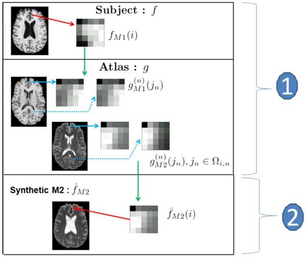
• To synthesize i^th patch f̂_M1(i) in f̂_M1, find the “best matching patches” $g_{M1}^{\left(n\right)}\left(j_n\right),j_n\in {\Omega }_{i,n}$ from $g_{M1}^{\left(n\right)},n=1,\dots ,N$ by searching the image domains Ω_gⁿ to solve Eqn. 3 (1 in Fig. 2).

• Construct the i^th patch in f̂_M1 as a non-local weighted average of $g_{M2}^{\left(n\right)}\left(j_n\right)’\mathrm{s}$ as shown in Eqn. 5 (2 in Fig. 2).

Figure 2.

Contrast synthesis algorithm flowchart : From the subject T1w image f_T1 we take the i^th patch f_T1(i) and identify the “best matching patches” from the atlases g⁽ⁿ⁾ as $\{g_{T1}^{\left(n\right)}\left(j_n\right);j_n\in {\Omega }_{i,n}\subset {\Omega }_{g^n}\}$. The corresponding patches from the T2w images $\{g_{T2}^{\left(n\right)}\left(j_n\right);j_n\in {\Omega }_{i,n}\}$ are combined using a non-local means approach¹⁸ to generate the synthetic T2 patch f̂_T2(i). The merging of all such patches generate the synthetic T2w image f̂_T2.

2.3 Resolution Enhancement

We merge the learning based image hallucination idea^{12, 17} to our tissue contrast synthesis approach to synthesize different contrast as well as improve resolution. To synthesize a high-resolution M2 image F̂_M2 from a low-resolution M1 image f_M1, Eqn. 2 is re-written as,

$${\widehat{F}}_{M2}\left(i\right)=ℱ\left\{G_{M2}^{\left(n\right)}\left({ℐ}_n\right)\right\},$$ (7)

with

$${ℐ}_n={𝒟}^{-1}\left({𝒥}_n\right),$$ (8)

where 𝒥_n is obtained from Eqn. 3. 𝒟⁻¹ takes the low-resolution patch from Ω_gⁿ to the high-resolution domain Ω_Gⁿ. This approach is similar to the example based super-resolution algorithms^{12, 14}, except that we are using patches from a different tissue contrast image $G_{M2}^{\left(n\right)}$.

3. RESULTS

3.1 Contrast Synthesis Validation on Brainweb

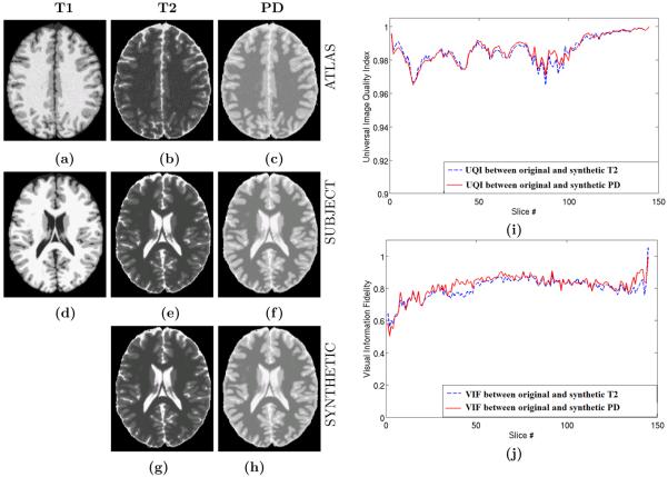
We use the Brainweb phantom²⁰ to validate the contrast synthesis method. M1 is chosen as T1w (Fig. 3(d)), and its original T2w and PDw acquisitions shown in Fig. 3(e)-(f). For all our experiments, we choose N = 1. The atlas is another set of phantoms, consisting of one of each of T1w, T2w, and PDw acquisitions, as shown in Fig. 3(a)–(c). Because the image intensities are taken from a codebook, the mean square error between the original and the reconstructed image is not a meaningful measure of performance. Instead, we use normalized mutual information (NMI), a visual information fidelity metric²¹ (VIF), and a universal image quality index²² (UQI) to quantify similarity between the original and the synthetic images. The NMI between two images A and B is defined as $\mathrm{NMI}(A,B)=\frac{2H(A,B)}{H\left(A\right)+H\left(B\right)}$ where H(A) is the entropy of the image A and H(A, B) is the joint entropy between A and B, with H(A, A) = H(A). We want low NMI values between the original and the synthetic images. Ideally, the synthetic image should give an accurate representation of the original image, which implies a small joint entropy between them.

Figure 3.

Brainweb Validation : (a) T1 Atlas, (b) T2 Atlas, (c) PD Atlas, (d) Test T1, (e) true test T2, (f) true test PD, (g) synthetic T2 from test T1, (g) synthetic PD from test T1, (i) Universal Image Quality Index²¹ between original and synthetic T2/PD, (j) Visual Information Fidelity²² between original and synthetic T2/PD. Normalized Mutual Information (NMI) between (e) and (g) is 0.7464 while NMI between (f ) and (h) is 0.7597.

The NMI between original T2 and synthetic T2 is 0.7464, while it is 0.7597 between the original PD and the synthetic one. VIF and UQI take two 2D images and return a number between 0 and 1. 1 is achieved only when the images are same or one is a scalar multiple of another. We plot UQI and VIF metrics in Fig. 3(i)-(j) for each slice of the 3D volumes between original and the synthetic T2 and PD. It is observed that the similarity is high on average.

3.2 Contrast Synthesis on Real Data

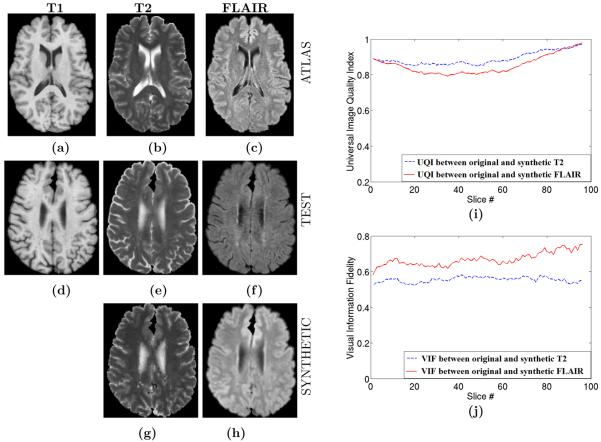
We use our algorithm to synthesize T2 and FLAIR images of a normal subject from its T1w SPGR acquisition for which we also have the actual T2 and FLAIR available for comparison. Fig. 4(a)-(c) show the T1, T2 and FLAIR images of another subject, which is used as the atlas. Fig. 4(g)-(h) show the synthetic T2 and FLAIR of the test subject in Fig. 4(d)-(f). Fig. 4(f) shows that the atlas FLAIR has a better contrast in GM-WM boundary compared to the test FLAIR. This is reflected in the synthetic FLAIR also. This highlights the benefit of our method, where a new contrast is created from the atlas, instead of the contrast reconstruction from the test image.

Figure 4.

Contrast Synthesis on Real Data : (a) T1 Atlas, (b) T2 Atlas, (c) FLAIR Atlas, (d) Test T1, (e) true test T2, (f) true test FLAIR, (g) synthetic T2, (g) synthetic FLAIR, (i) Universal Image Quality Index²¹ between original and synthetic T2/FLAIR, (j) Visual Information Fidelity²² between original and synthetic T2/FLAIR for each slice of the volume. Normalized Mutual Information (NMI) between (e) and (g) is 0.7464 while NMI between (f) and (h) is 0.7597. The atlas FLAIR has a better contrast in GM-WM boundary compared to the subject FLAIR. As a consequence, the synthetic FLAIR has better GM-WM contrast than the subject. This highlights the benefits of our method. As the synthetic image intensities are taken from the atlas, a new contrast is “created”.

The NMI between the original and the reconstructed T2 and FLAIR are 0.3697 and 0.3102, respectively. NMI, being a distribution dependent statistic, is sensitive to the actual distribution of the intensities rather than the contrast. The NMI numbers for the phantom validation are larger than those of the real data, because the Brainweb phantoms have widely different histograms while keeping the same contrast, while the real data have similar histograms. The plot of UQI and VIF for each slice is also shown in Fig. 4(i)-(j).

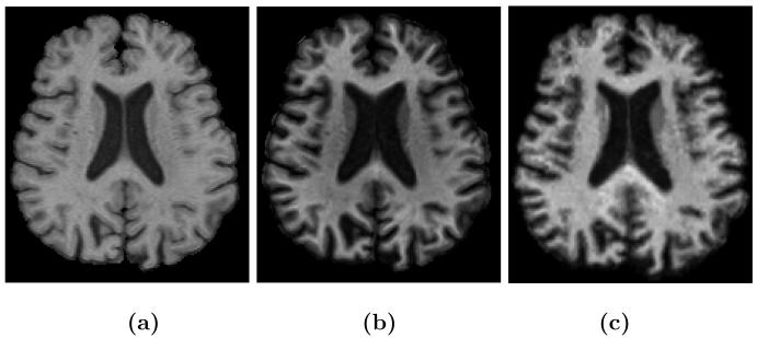
The next experiment on real data consists of synthesizing an MPRAGE image from its SPGR acquisition of the same resolution, because MPRAGE images are of importance for their superior GM-WM contrast. The required atlas consists of a pair of SPGR and MPRAGE acquisitions of another subject. Fig. 5(a)-(b) shows the true SPGR and true MPRAGE acquisitions, with Fig. 5(c) being the same resolution synthetic MPRAGE image. The NMI between the original MPRAGE and the synthetic MPRAGE is 0.3254, while it is 0.3341 between the original MPRAGE and the original SPGR.

Figure 5.

Contrast Change, from SPGR to MPRAGE: (a) a T1w spoiled gradient recalled (SPGR) acquistion, (b) its true magentization prepared rapid gradient echo (MPRAGE) acquistion of same resolution, (c) a synthetic MPRAGE of same resolution as the SPGR. Normalized mutual information between them is 0.3254, while it is 0.3341 between the SPGR and the true MPRAGE.

3.3 Contrast Synthesis with Resolution Enhancement

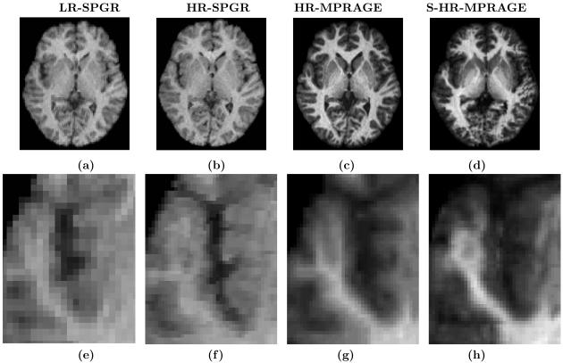
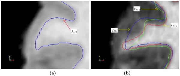
We show that using both contrast synthesis and resolution enhancementment leads to improved delineation of cortical surfaces. We use M1 as SPGR and M2 as MPRAGE. MPRAGE images, having superior GM-WM contrast, are a better candidate for the delineation of the inner cortical surface compared to SPGR images. So in the absence of an MPRAGE image, we could synthesize one, thus enabling better delineation. Our data set contains a 1.875×1.875×3 mm low-resolution (LR) SPGR image f_M1, its high resolution (HR) 0.9375×0.9375 1.5 mm true MPRAGE acquisition F_M2 and true HR SPGR acquistion F_M1, shown in Fig. 6(a)-(c), respectively. Using Eqn. 7, a HR MPRAGE image F̂_M2 is generated, shown in Fig. 6(d). The cortical inner surfaces are found using CRUISE²³. For comparison, “the best available truth” or a “reference” standard of the inner surface is obtained from F_M2, with which we compare the surface obtained from F̂_M2 and F_M1. Fig. 7(a) and (b) show how the lack of GM-WM contrast gives rise to a poor cortical inner surface reconstruction for F_M1 when compared to the reference “true” reconstruction from F_M2 and the reconstruction from our method, F̂_M2. Table 1 shows that the mean differences for four subjects between their inner surfaces as generated from F̂_M2 and F_M1 as compared to F_M2. The smaller differences show our super-resolution approach gives a marginal improvement in the delineation of the inner surface.

Figure 6.

Contrast Synthesis with Resolution improvement: (a) test LR SPGR image f_M1, (b) its HR SPGR acquisition F_M1, (c) HR MPRAGE acquisition F_M2, (d) our synthetic HR MPRAGE F̂_M2, The bottom row shows corresponding zoomed regions for each image in the top row.

Figure 7.

(a) Inner surface computed from high-resolution SPGR F_M1 (blue) overlaid on F_M1, (b) Inner surface computed from high-resolution MPRAGE F_M2 (red), synthetic high-resolution MPRAGE F̂_M2 (green) overlaid on F_M2.

Table 1.

Distance (in mm) between inner surfaces of reference image HR MPRAGE F_M2 with synthetic HR MPRAGE F̂_M2 and HR SPGR F_M1. MAD is the mean absolute distance, Std is standard deviation of the distance, Max is maximum distance.

		Subject
		1	2	3	4
MAD	F M1	1.2245	1.1567	1.3991	1.2213
	F̂ M2	0.9522	1.1038	0.9915	1.2308
Std	F M1	0.8911	1.0123	1.2139	0.4587
	F̂ M2	0.7966	1.0338	1.1001	0.6738
Max	F M1	11.4512	7.7123	8.9012	15.1121
	F̂ M2	7.0642	12.3681	6.6370	13.1400

4. DISCUSSION AND CONCLUSION

The similarity criteria in Eqn 3 is chosen to be the L² norm, the underlying assumption being the intensities of f and $g_{M1}^{\left(n\right)}$ differ by a Gaussian noise, or they follow a similar distribution. If the intensity distributions are different, then L² norm fails to produce correct matches from Eqn. 3. Also, we used one atlas for our experiments, but we believe using more than one atlas helps in finding more accurate J_n. Involving more complex similarity criteria like gradient or texture into Eqn. 3 will also produce more accurate J_n. Some of the parameters, like λ in Eqn. 3 or β in Eqn. 6 are required to be estimated by cross-validation. Also, the smoothness of the image depends on the amount p% of “best matching patches” used, which also needs to be estimated by cross validation.

In summary, we proposed an atlas based image synthesis technique to generate different MR tissue contrasts from a single image acquisition. It is essentially a patch-matching algorithm where a template patch from a test image is matched onto a multi-modal multi-resolution atlas and patches from the atlas are used to generate a synthetic alternate tissue contrast high resolution image. The contribution of this method is that new MR contrasts can be synthesized from the atlas, and unlike histogram matching, this method uses local contextual information to synthesize images. We have validated our method on Brainweb phantoms, and showed that T2, PD, and FLAIR images can be generated from a single T1w acquisition. We also demonstrated that a synthetic high-resolution MPRAGE image can be generated from its low-resolution SPGR acquisition, which leads to improved cortical segmentation. So far our experiments have been carried out on normal subjects. Future work includes reconstruction of alternate tissue contrasts like T2 and FLAIR on patients with lesions.

REFERENCES

- 1.Dale AM, Fischl B, Sereno MI. Cortical Surface-Based Analysis i: Segmentation and Surface Reconstruction. NeuroImage. 1999;9(2):179–194. doi: 10.1006/nimg.1998.0395. [DOI] [PubMed] [Google Scholar]
- 2.Bazin PL, Pham DL. Topology-Preserving Tissue Classification of Magnetic Resonance Brain Images. IEEE Trans. on Med. Imag. 2007;26(4):487–498. doi: 10.1109/TMI.2007.893283. [DOI] [PubMed] [Google Scholar]
- 3.Clarke LP, Velthuizen RP, Phuphanich S, Schellenberg JD, Arrington JA, Silbiger M. MRI: Stability of Three Supervised Segmentation Techniques. Mag. Res. in Med. 1993;11(1):95–106. doi: 10.1016/0730-725x(93)90417-c. [DOI] [PubMed] [Google Scholar]
- 4.Fischl B, Salat DH, van der Kouwe AJW, Makris N, Segonne F, Quinn BT, Dale AM. Sequence-independent Segmentation of Magnetic Resonance Images. NeuroImage. 2004;23:S69–S84. doi: 10.1016/j.neuroimage.2004.07.016. [DOI] [PubMed] [Google Scholar]
- 5.Hong X, McClean S, Scotney B, Morrow P. Model-Based Segmentation of Multimodal Images. Comp. Anal. of Images and Patterns. 2007;4672:604–611. [Google Scholar]
- 6.Souplet J, Lebrun C, Ayache N, Malandain G. An Automatic Segmentation of T2-FLAIR Multiple Sclerosis Lesions. Midas Journal, MICCAI Workshop. 2008 [Google Scholar]
- 7.Hunt BR. Super-Resolution of Images: Algorithms, Principles, Performance. Intl. Journal of Imag. Sys. and Tech. 1995;6(4):297–304. [Google Scholar]
- 8.Park S, Park M, Kangg MG. Super-resolution Image Reconstruction: A Technical Overview. IEEE Signal Proc. Mag. 2003;20(3):21–36. [Google Scholar]
- 9.Sun J, Zheng NN, Tao H, Shum H. Image Hallucination with Primal Sketch Priors. IEEE Conf. Comp. Vision and Patt. Recog. 2003;2:729–736. [Google Scholar]
- 10.Jia K, Gong S. Hallucinating Multiple Occluded Face Images of Different Resolutions. Patt. Reco. Letters. 2006;27:1768–1775. [Google Scholar]
- 11.Baker S, Kanade T. Hallucinating faces. IEEE Intl. Conf. on Automatic Face and Gesture Recog. 2000:83–88. [Google Scholar]
- 12.Freeman WT, Jones TR, Pasztor EC. Example-Based Super-Resolution. IEEE Comp. Graphics. 2002;22(2):56–65. [Google Scholar]
- 13.Xiong Z, Sun X, Wu F. Image Hallucination with Feature Enhancement. IEEE Conf. on Comp. Vision and Patt. Recog. 2009:2074–2081. [Google Scholar]
- 14.Rousseaui F. Brain Hallucination. European Conf. on Comp. Vision. 2008;5302:497–508. [Google Scholar]
- 15.Ma L, Wu F, Zhao D, Gao W, Ma S. Learning-Based Image Restoration for Compressed Image through Neighboring Embedding. Advances in Multimedia Info. Proc. 2008;5353:279–286. [Google Scholar]
- 16.Ng M, Shen H, Lam E, Zhang L. A Total Variation Regularization Based Super-Resolution Reconstruction Algorithm for Digital Video. EURASIP Journal on Advances in Signal Proc. 2007;74585 [Google Scholar]
- 17.Fan W, Yeung DY. Image Hallucination Using Neighbor Embedding over Visual Primitive Manifolds. IEEE Conf. Comp. Vision and Patt. Recog. 2007:17–22. [Google Scholar]
- 18.Buades A, Coll B, Morel JM. A Non-Local Algorithm for Image Denoising. IEEE Comp. Vision and Patt. Recog. 2005;2:60–65. [Google Scholar]
- 19.Gasser T, Sroka L, Steinmetz C. Residual Variance and Residual Pattern in Nonlinear Regression. Biometrika. 1986;73:625–633. [Google Scholar]
- 20.Cocosco C, Kollokian V, Kwan R-S, Evans A. Brainweb: Online Interface to a 3D MRI Simulated Brain Database. NeuroImage. 1997;5(4):S425. [Google Scholar]
- 21.Sheikh H, Bovik A, de Veciana G. An Information Fidelity Criterion for Image Quality Assessment using Natural Scene Statistics. IEEE Trans. on Image Proc. 2005;14(12):2117–2128. doi: 10.1109/tip.2005.859389. [DOI] [PubMed] [Google Scholar]
- 22.Wang Z, Bovik AC. A Universal Image Quality Index. IEEE Signal Proc. Letters. 2002;9(3):81–84. [Google Scholar]
- 23.Han X, Pham D, Tosun D, Rettmann M, Xu C, Prince J. Cruise: Cortical reconstruction using implicit surface evolution. NeuroImage. 2004;23:997–1012. doi: 10.1016/j.neuroimage.2004.06.043. [DOI] [PubMed] [Google Scholar]