Identification of N-Glycan Serum Markers Associated with Hepatocellular Carcinoma from Mass Spectrometry Data

Abstract

Glycocylation represents the most complex and widespread post-translational modifications in human proteins. The variation of glycosylation is closely related to oncogenic transformation. Therefore, profiling of glycans detached from proteins is a promising strategy to identify biomarkers for cancer detection. This study identified candidate glycan biomarkers associated with hepatocellular carcinoma by mass spectrometry. Specifically, mass spectrometry data were analyzed with a peak selection procedure which incorporates multiple random sampling strategies with recursive feature selection based on support vector machines. Ten peak sets were obtained from different combinations of samples. Seven peaks were shared by each of the 10 peaksets, in which 7–12 peaks were selected, indicating 58–100% of peaks were shared by the 10 peaksets. Support vector machines and hierarchical clustering method were used to evaluate the performance of the peaksets. The predictive performance of the seven peaks was further evaluated by using 19 newly generated MALDI-TOF spectra. Glycan structures for four glycans of the seven peaks were determined. Literature search indicated that the structures of the four glycans could be found in some cancer-related glycoproteins. The method of this study is significant in deriving consistent, accurate, and biological significant glycan marker candidates for hepatocellular carcinoma diagnosis.

1. Introduction

As the most complex and widespread post-translational modification (PTM),¹ glycosylation plays crucial roles during different oncogenetic processes.^2-4 Many important tumor markers, such as CEA,⁵ CA125,⁶ and PSA,^7-9 are glycoproteins with altered glycan profiles in cancer. As one of the most common types of malignant tumor, hepatocellular carcinoma (HCC) is difficult to diagnose due to the highly heterogenic nature of the disease and has a low survival rate once diagnosed.¹⁰ The popular method to diagnose HCC is to measure a serum glycoprotein marker alpha-fetoprotein (AFP). However, this marker has limited sensitivity (41–65%).¹¹ This sensitivity could be improved by measuring several highly specific glycoprotein markers.¹¹ Therefore, there is an urgent need to discover additional markers associated with HCC for the early diagnosis.

Currently, glycan marker discovery by analyzing mass spectrometry (MS) data presents great potential to identify a panel of biomarkers relevant for early diagnosis of heterogenic diseases with improved accuracies.^12-15 However, this approach is characterized by high dimensionality and complex patterns with a substantial amount of noise arising from measurement deviation, disease heterogeneity, and biological variability. A robust computational method is required to identify markers relevant to a particular problem from the MS data sets. Machine learning methods, especially neural networks and support vector machines (SVM), provide potential application in the marker selection from MS data. Using shallow feature selection method and Bayesian neural network (BNN) classifier, 99% sensitivity and 98% specificity were reached on the SELDI-TOF MS data to identify ovarian cancer using 2-fold cross validation (CV).¹² Information gain and SVM classifier were used for prion disease diagnosis from MALDIFTMS data and yielded 72% sensitivity and 73% specificity by leave-one-out cross validation (LOOCV).¹³ t-test and several classification methods such as discriminant analyses, k-nearest neighbor analysis, and SVM were used for identifying ovarian cancer cases from normal patients, and SVM have resulted in the lowest error rates.¹⁵ These methods utilized a filter strategy which identifies relevant peaks independent of the classifiers. In the feature selection from machine learning classifiers, another popular strategy is wrapper method, where classifiers that built from different peak subsets evaluate the goodness of peak subsets by such criteria as CV error rate or accuracy from the validation data set; the wrapper method presented good performance and a stable feature subset when applied in microarray gene discovery¹⁶ and can be extended into MS peak selection. Mahadevan et al. built a feature selection method known as recursive feature elimination-support vector machine (RFE-SVM) to separate pneumonia from healthy people by mass spectrometry. They obtained an overall accuracy of 84–96% by 4-fold CV and 87–97% by LOOCV, providing much better predictive performance when compared with multivariate analysis methods.¹⁷

In our previous studies, we utilized ant colony optimization combined with support vector machines (ACO-SVM) peak selection to identify biomarkers for HCC diagnosis^14,18-21 using matrix-assisted laser desorption/ionization time-of-flight mass spectrometry (MALDI-TOF MS). Six peptide markers were identified that yielded 100% sensitivity and 91% specificity in an independent test set,^14,21 and two of them were found to be fragments of Complement C3 and C4.^14,21 Six to 10 glycan markers were found to be associated with HCC with 87–93% sensitivity and 89–100% specificity.^14,18-20 Two glycans with permethylated molecular weight at 2040 and 4502 were identified in most of these studies.^14,19,20 In this study, we apply an integrated RFE-SVM approach to select glycan markers correctly distinguishing HCC cases from chronic liver disease (CLD) patients through MALDI-TOF MS data. This method incorporated RFE-SVM with the consensus scoring system, multiple random sampling method, and feature-ranking consistency evaluation system. We generated 10 discriminant peak sets from the various combinations of MALDI-TOF spectra. Each set contained 7–12 peaks; 7 glycan peaks were present in all 10 peak sets, indicating that 58–100% of all the peaks in the 10 sets were shared by all of them. These results suggest that the discriminant peaksets are insensitive to the sample combinations. Different evaluation methods and a newly generated data set were used to evaluate the performances of the selected peaks. Among previously selected candidate markers, those with permethylation molecular weight at 2040, 2186, and 4502^14,18-20 were included in the 7 peaks which were selected by all of the 10 sets. The structures of 4 glycans of the 7 peaks were determined. A literature search indicated that the structures of the four glycans could be found in cancer-related glycoproteins beta-glucuronidase, cytochrome, and immunoglobulin, suggesting their possible roles in cancer progression.

2. Materials and Methods

Data Sets

Two hundred and three serum samples were collected from 73 HCC cases, 52 CLD cases, and 78 healthy individuals from Cairo, Egypt.¹⁴ Diagnosis of HCC was confirmed by pathology, cytology, imaging, and serum AFP. CLD cases included fibrosis and cirrhosis patients. Controls were recruited among patients from an orthopedic and fracture clinic and were frequency-matched to cancer cases by gender, age, and smoking status.¹⁴

N-Glycans were released from glycoprotein, extracted, and permethylated by a solid-phase approach. The resulting permethylated glycans were spotted on a MLADI plate with DHB-matrix, and the MALDI plate was dried under vacuum. Mass spectra were acquired using a 4800 MALDI TOF/TOF Analyzer (Applied Biosystems, Inc.) equipped with a Nd:YAG 355-nm laser. MALDI spectra were recorded in positive-ion mode, since permethylation eliminates the negative charge normally associated with sialylated glycans.

Two hundred and three mass spectra, including 73 HCC cases, 52 CLD cases and 78 healthy individuals, were acquired at the National Center for Glycomics and Glycoproteomics at Indiana University. The 73 HCC spectra and 52 CLD spectra were utilized for peak selection. Nineteen additional spectra were generated at the Proteomics and Metabolomics Shared Resource at Georgetown University Medical Center and used for peak evaluation. The 19 spectra were obtained from 9 CLD and 10 HCC samples, which are a subset of the previously analyzed 52 CLD and 73 HCC cases. The same sample preparation protocol¹⁴ was used in generating the original 203 spectra and the additional 19 spectra.

Glycan Structure Determination

Structural assignment of the different N-glycans was achieved through high-energy collision incident dissociation (CID) tandem MS analyses. Although tandem MS analysis utilizing high energy CID is currently allowing comprehensive characterization of glycan structures, enzymatic sequencing, in some cases, is deemed necessary to confirm structural attributes such as linkages. This is accomplished by employing an array of excoglycosidases including those specific for different sialic acid, fucose and galactose linkages. For enrichment of minor glycans, we first used the quantification by TOF-MS to select samples with the highest intensity of a glycan of interest. The glycan is then further enriched from these samples by micro fractionation, as described previously.^22,23 Briefly, our method for separation of the permethylated glycans incorporates derivatization, C18 trapping of permethylated glycans, and C18 nano-LC separation.²² The chromatographic separation of permethylated glycans is attained initially using an isocratic condition of 32% phase B (acetonitrile containing 0.1% formic acid) for 40 min, followed by an increase of phase A to 55% over 15 min. The mobile composition is then held at 55% for 10 min. Phase A consists of 3% aqueous acetonitrile with 10 mM ammonium formate. The separation is achieved on C18 nanocolumn (150 × 0.075 mm fused silica pulled-tip column).

MALDI-TOF MS Data PreProcessing

Each spectrum of the 203 MALDI sample consisted of approximately 121 000 data points in the mass range of 1500–5500 Da. To reduce their dimension, the spectra were first binned with the size of 0.2 Da. The mean of the intensities within each bin was used as the intensity variable. Using this binning method, the dimension of each spectrum was reduced to 20 000. Baseline-corrected spectra were then used to indentify peaks by using a wavelet-based peak detection method.²⁴ After peak identification, the spectra were normalized with the highest peak as 100 and the lowest peak as 0.

After the alignment of the 203 mass spectra from the peak lists,²⁵ 3397 peaks were identified. Since there are artifacts in the aligned intensity, the intensity of each aligned m/z value was treated as the maximum intensity in the original spectra within ±0.5 Da. The average intensities of the aligned peaks were used to determine possible clusters of isotopic distributions. With this approach, the number of peaks was further reduced to 447 assuming that each isotopic cluster contains only one glycan molecule. The 447 peaks were utilized to build classifiers and to select the most discriminant peaks.

Classification Method

Support vector machines (SVM), a supervised machine learning method proposed by Vapnik, was used in this study as the classification tool.²⁶ SVM-based classifiers are shown to prove excellent classification performance and have been successfully applied in microarray data analysis¹⁶ and mass spectrometry data analysis.^27,28

There are two types of SVM: linear and nonlinear. In linear SVM, a hyperplane in the feature space is directly constructed. This hyperplane, which separates two different classes of feature vectors with a maximum margin, is generated by finding a vector w and a variable b that minimizes ∥w∥², which satisfies the following conditions: w · x_i + b ≤ −1, for y_i = −1 (cancer patients) and w · x_i + b ≤ −1, for y_i = −1 (noncancer people). Here, x_i is a feature vector, y_i is the group index, w is a vector normal to the hyperplane, |b|/∥w∥ is the perpendicular distance from the hyperplane to the origin, and ∥w∥ is the Euclidean norm of w. This optimization problem can be described as to minimize 0.5∥w∥² subject to y_i(w · x_i + b) ≥ 1. With the introduction of Lagrangian multiplier a_i, this problem can be rewritten as $L_P(w,b,a)=0.5{\Vert w\Vert }^2-{\Sigma }_{i=1}^n{a}_i(y_i(x_i\cdot w+b)-1)$ where α_i ≥ 0, and efficiently solved by maximizing $L_D\left(a\right)={\Sigma }_{i=1}^n{a}_i-0.5{\Sigma }_{i,j=1}^n{a}_i{a}_j{y}_i{y}_j\left(x_i\cdot x_j\right)$ under the constraints ${\Sigma }_{i=1}^n{a}_i{y}_i=0$ and α_i ≥ 0, i = 1, 2, …, n. After the determination of w and b, a given vector x can be classified by using sign [(w · x) + b]. A positive or negative value indicates that the vector x belongs to the positive or negative class, respectively.

Nonlinear SVM, by using a kernel function, projects both positive and negative examples into a higher-dimensional feature space and then the linear SVM procedure can be applied to the feature vectors in this feature space. In our experiments, Gaussian kernel K(X,X′) = exp (−(∥X − X′∥)/(2σ²)) was used since this kernel performs similar with linear kernel and sigmoid kernel under certain parameters,^29-31 and few parameters were needed to be tuned when comparing with the polynomial kernel.

The performance of SVM classification can be measured by true positive TP (number of cancer patients correctly predicted as cancer patient), false negative FN (number of cancer patients incorrectly predicted as noncancer people), true negative TN (number of noncancer people correctly predicted noncancer people), and false positive FP (number of noncancer people incorrectly predicted as cancer patients). Three indicators, sensitivity Q_p = TP/(TP + FN), specificity Q_n = TN/(TN + FP), and overall accuracy Q = (TP + TN)/(TP + FN + TN + FP), were used to measure the predictive performance.

Peak Selection Method

The recursive feature elimination-SVM (RFE-SVM) method has been successfully used for feature selection from high dimensional microarray and mass spectrometry data.^16,27,28 Briefly, RFE-SVM uses the prediction accuracy from SVM to assess the goodness of each peak and to determine a peak ranking. The peak ranking criterion of RFE-SVM is based on the change in the objective function upon removing each peak. This objective function can be represented by a cost function J = 0.5a^THa − a^T1, where H is the matrix with elements H(i,j) = y_iy_jK(x_i,x_j), computed by using the training set only. When a given peak k is removed or its weight w_k is reduced to zero, the change in the cost function J(k) is given by DJ(k) = 0.5(∂²J/∂w_k²)(Dw_k)². The change in weight Dw_k=w_k−0 corresponds to the removal of peak k. Hence, the change in the cost function can be written as DJ(k) = 0.5a^THa−0.5a*^TH(−k)a*, where H is the matrix with elements y_iy_jK(x_i,x_j). H(−k) is the matrix computed by using the same method as that of matrix H but with its kth component removed. For the sake of complicity and to reduce computational complexity, α* is supposed to be equal to α, under the assumption that the removal of one peak will not significantly influence the values of αs. The change in the cost function indicates the contribution of the peak to the decision function and serves as an indicator of peak ranking position.

Peak Elimination Procedure

To present statistical meaning, peak selection is conducted based on a multiple random sampling strategy. Each random sampling divides all MALDI-TOF spectra into a training set that contains half of the samples and an associated test set, which contains the remaining half. By using this random sampling strategy, 5000 training-test sets, each containing a unique combination of samples, are generated. These 5000 training-test sets are randomly divided into 10 sampling groups, with 500 training-test sets in each group (Figure 1). Every sampling group is then used to derive a signature by RFE-SVM.

Figure 1.

Overview of the peak selection procedure.

In every training-test sampling group generated by multiple random sampling, each training set (totally 500 training sets) is used to train a SVM class-differentiation system and the peaks are ranked by using RFE according to the contribution of peaks to the SVM classifier. The performance of each peak subset which selected in every iteration step is evaluated on the associated 500 test sets. Two typical variables used in RBF kernel, σ and C, are kept constant during all iterations in the peak elimination procedure and among all the 500 training set in this group, in order to derive a peak ranking criterion consistent for all iterations and different combination of samples. Different combinations of variables σ and C are scanned. One combination of the two variables can be defined as a universal set of globally optimized variables, if the best average class differentiation accuracy over the 500 test sets in this group is achieved by a SVM class differentiation system using these variables and on a peak subset which selected in a certain iteration step. The peak subset can be determined as one discriminant peak set.

To further reduce the chance of erroneous elimination of predictor-peaks, additional peak-ranking consistency evaluation steps are implemented on top of the normal RFE procedures in each group:

• (1) For every training-set, subsets of peaks ranked in the bottom (which give least contribution to the SVM classification procedure) with combined score lower than the first few top-ranked peaks (which give highest contribution to the SVM classification procedure) are selected such that collective contribution of these peaks less likely outweighs the top-ranked ones.

• (2) For every training-set, the step (1) selected peaks are further evaluated to choose those not ranked in the upper 50% in previous iteration so as to ensure that these peaks are consistently ranked lower.

• (3) A consensus scoring scheme is applied to peaks selected in step (2) such that only those appearing in most of the 500 testing-sets were eliminated.

For each sampling group, different SVM parameters are scanned, various RFE iteration steps are evaluated to identify the globally optimal SVM parameters and RFE iteration steps that give the highest average class-differentiation accuracy for the 500 testing-sets. The 10 discriminant peak sets derived from these sampling-groups are then applied to evaluate the stability and performance.

Computational Complexity Estimation

The computational complexity of SVM is of O(nm²) where m is the number of training samples and n is the number of peaks. In the feature selection procedure, SVM will be retrained many times with a decreasing number of features. The number of iterations is n if we remove the peaks one by one. When the multiple randomly sampling strategies are applied, the RFE-SVM needs to be executed l times, where l is the number of training sets used in each sampling group. Hence the overall computational complexity is O(ln²m²).

3. Results and Discussion

The 203 MALDI glycan spectra were obtained from 73 HCC cases, 52 CLD cases, and 78 healthy samples from Egyptian population.¹⁴ The 52 CLD cases included 21 fibrosis patients, 25 cirrhosis patients, and 6 patients with unknown clinical information. Each mass spectrum contained approximately 121 000 data points in the mass range of 1500–5500 Da. After the preprocessing procedure of binning, baseline correction, peak identification, and peak alignment, the dimension of glycan spectra was reduced to 3397 m/z peaks.

The average intensities of the 3397 peaks in 203 spectra were used to determine a cluster of peaks that can represent an isotopic distribution. Figure 2 shows the average peak intensities of the 203 spectra in the mass range from 2800 to 2900. A close examination of the peaks in the figure reveals that individual glycans are represented by a cluster of peaks. This is due to the high resolution MALDI-TOF instrument used in this study that has the capability to resolve isotopes of individual glycans. We assumed that each cluster contains only one glycan molecule in order to simplify the problem, and reduced the number of peaks to 447 by selecting the local maximum peaks.

Figure 2.

Average peak intensities from 203 glycan MALDI spectra (a snapshot of m/z ranges from 2800 to 2900). Local maximum points (marked by star) were used in subsequent analyses assuming that they adequately represent clusters of peaks that may be an isotopic distribution of individual glycans.

Hierarchical clustering analysis³² based on the 447 peaks grouped the 203 samples into three clusters (Table 1). The first cluster was dominated by HCC samples; it included 67 HCC, 4 CLD and 27 healthy samples. We call this cluster HCC Cluster. The second cluster, named as CLD Cluster, was dominated by CLD cases, including 3 HCC, 24 CLD and 14 healthy samples. The third cluster, named as Healthy Cluster, contained 3 HCC, 24 CLD and 37 healthy samples. Ninty-two percent of the HCC samples were found in the HCC Cluster, whereas 92% of the CLD samples and 65% of the healthy samples were present in the CLD or the Healthy Clusters, respectively. These results suggest that the 447 peaks have a certain discriminating ability to differentiate cancer patient from noncancer individuals (CLD and healthy) through an unsupervised clustering method.

Table 1.

Results from Linkage Hierarchical Clustering Analysis by Using the Each of the 10 Peak Sets We Obtained and the 7 Most Frequently Selected Peaks^a

		number of samples in each cluster (percentage in the sample group)
peak sets (number of peaks)	sample groups	HCC cluster	CLD cluster	healthy cluster
447 peaks (447)	HCC	67 (92%)	3 (4%)	3 (4%)
	CLD	4 (8%)	24 (46%)	24 (46%)
	Healthy	27 (35%)	14 (18%)	37 (47%)
Peak set 1 (9)	HCC	72 (99%)	0 (0%)	1 (1%)
	CLD	0 (0%)	36 (69%)	16 (31%)
	Healthy	12 (15%)	16 (21%)	50 (64%)
Peak set 2 (9)	HCC	69 (95%)	0 (0%)	4 (5%)
	CLD	0 (0%)	32 (62%)	20 (38%)
	Healthy	9 (11%)	14 (18%)	55 (71%)
Peak set 3 (12)	HCC	70 (96%)	0 (0%)	3 (4%)
	CLD	0 (0%)	25 (48%)	27 (52%)
	Healthy	10 (13%)	10 (13%)	58 (74%)
Peak set 4 (11)	HCC	72 (99%)	0 (0%)	1 (1%)
	CLD	0 (0%)	37 (71%)	15 (29%)
	Healthy	9 (11%)	20 (26%)	49 (63%)
Peak set 5 (11)	HCC	71 (97%)	0 (0%)	2 (3%)
	CLD	0 (0%)	32 (62%)	20 (38%)
	Healthy	12 (15%)	17 (22%)	49 (63%)
Peak set 6 (9)	HCC	69 (95%)	0 (0%)	4 (5%)
	CLD	0 (0%)	32 (62%)	20 (38%)
	Healthy	9 (11%)	14 (18%)	55 (71%)
Peak set 7 (7)	HCC	66 (90%)	0 (0%)	7 (10%)
	CLD	0 (0%)	48 (92%)	4 (8%)
	Healthy	7 (9%)	21 (27%)	50 (64%)
Peak set 8 (9)	HCC	70 (96%)	0 (0%)	3 (4%)
	CLD	0 (0%)	26 (50%)	26 (50%)
	Healthy	8 (10%)	8 (10%)	62 (80%)
Peak set 9 (7)	HCC	66 (90%)	0 (0%)	7 (10%)
	CLD	0 (0%)	48 (92%)	4 (8%)
	Healthy	7 (9%)	21 (27%)	50 (64%)
Peak set 10 (9)	HCC	70 (96%)	0 (0%)	3 (4%)
	CLD	0 (0%)	47 (90%)	5 (10%)
	Healthy	13 (16%)	10 (13%)	55 (71%)
7 peaks selected by all 10 sets (7)	HCC	66 (90%)	0 (0%)	7 (10%)
	CLD	0 (0%)	48 (92%)	4 (8%)
	Healthy	7 (9%)	21 (27%)	50 (64%)

^aFor each of the three clusters, the sample group with the highest number of samples is marked in boldface.

Using supervised SVM classifier and 447 peaks through the LOOCV evaluation method, 95% accuracy to separate HCC from CLD samples and 96% accuracy to separate HCC from noncancer samples (CLD and healthy) were achieved. These results suggest that the 447 peaks could perform perfectly in separating HCC from CLD or healthy individuals by supervised analysis.

To determine the peaks most pertinent to differentiating HCC spectra from CLD spectra, 10 peak subsets were obtained using integrated RFE-SVM from 5000 training-test data sets with 447 peaks. These 5000 training-test data sets were generated through a random sampling method, with each training set containing 36–37 HCC and 26–27 CLD, and their associated test set consisting of the remaining HCC and CLD samples (36–37 HCC and 25–26 CLD). These data sets were divided into 10 groups, with 500 training-test data set in each group. For each group, one peakset was obtained. Subsequently, totally 10 peaksets were generated. There were 7 to 12 peaks for each peak set. The stability of the peak sets was estimated from the percentage of the peaks shared by all of the 10 peak sets. From Table 2, it is obvious that seven peaks were selected by all of the 10 peak sets. This indicates that 58–100% of all the peaks in each peak set were shared by all of 10 sets, suggesting that our method is quite stable. The overall accuracy ranging from 99.79 to 99.99% were obtained using the associated test sets (Table 2). We utilized backward elimination method, in which feature selection was started with the full-dimensional peakset (447 peaks) and sequentially deleted the least important peaks. We also applied forward elimination method, in which feature selection was started with an empty peakset and sequentially added the most important peaks, on the RFE-SVM with multiple randomly sampling strategy, ranking consistency evaluation, and consensus scoring system. Similar results can be obtained from both methods and the overall accuracies and consistency rates from both methods were significantly higher than those obtained using a typical RFE-SVM procedure (Table 3).

Table 2.

Predictive Accuracies Obtained by Using Each of the 10 Peak Sets Derived from This Work As Input to SVM Classifiers^a

peak sets	number of selected peaks in each set	accuracy from 500 test sets			peaks selected
		sensitivity	specificity	accuracy
Peak Set 1	9	99.99%	99.99%	99.99%	1580, 1996, 2040, 2187, 2192, 2851, 2893, 4311, 4502
Peak set 2	9	99.99%	99.95%	99.97%	1580, 1996, 2040, 2187, 2192, 2286, 2851, 4311, 4502
Peak Set 3	12	99.64%	100%	99.79%	1580, 1800, 1996, 2040, 2187, 2244, 2511, 2851, 4311, 4502, 4516
Peak Set 4	11	99.99%	99.98%	99.99%	1580, 1996, 2040, 2151, 2187, 2214, 2411, 2711, 2851, 4311, 4502
Peak Set 5	11	100%	99.97%	99.99%	1580, 1996, 2040, 2187, 2214, 2411,2490, 2851, 2511, 4311, 4502
Peak Set 6	9	99.99%	99.96%	99.98%	1580, 1996, 2040, 2187, 2192, 2286, 2851, 4311, 4502
Peak Set 7	7	99.99%	99.97%	99.98%	1580, 1996, 2040, 2187, 2851, 4311, 4502
Peak Set 8	9	99.90%	99.90%	99.90%	1580, 1800, 1996, 2040, 2187, 2411, 2851, 4311, 4502
Peak Set 9	7	100%	99.98%	99.99%	1580, 1996, 2040, 2187, 2851, 4311, 4502
Peak Set 10	10	100%	99.90%	99.96%	1580, 1996, 2040, 2187, 2411, 2851, 3604, 4311, 4502, 4516

^aResults were obtained by calculating the average prediction accuracy of 500 test sets for each peak set.

Table 3.

Predictive Performance and Consistency Rates of Peaksets by Using Different Peak Selection Procedures

procedure	number of peaks in 10 peaksets	number of peaks (percentage of peaks) selected by all 10 peaksets	accuracies of each peakset	peaks selected by all 10 peaksets
RFE-SVM with multiple randomly sampling strategy, ranking consistency evaluation, and consensus scoring system, backward elimination	7–12	7 (58–100%)	99.79–99.99%	1580, 1996, 2040, 2187, 2851, 4311, 4502
RFE-SVM with multiple randomly sampling strategy, ranking consistency evaluation, and consensus scoring system, forward elimination	4–9	4 (44–100%)	99.00–99.26%	2040, 2241, 2851, 4502
RFE-SVM, the number of features was reduced by a factor of 2 at every iteration	4–7	2(29~50%)	77.42–88.71%	1580, 2040

Hierarchical clustering analysis was performed on the 10 peak sets and 203 samples. The 78 samples from healthy individuals were not used in the peak selection procedure. Instead, they were employed in the evaluation step, together with the CLD and HCC samples. Table 1 shows the cluster analysis results obtained using the 10 peak sets derived in this study. Each peak set has the ability to stratify the samples into HCC Cluster, CLD Cluster and Healthy Cluster. HCC Clusters included 66–72 HCC, 0 CLD and 7–27 healthy samples. CLD Clusters included 0 HCC, 25–48 CLD and 10–21 healthy samples. Healthy Clusters included 1–7 HCC, 4–27 CLD and 49–62 healthy samples. These results indicate that 90–99% of HCC, 48–92% of CLD and 63–80% of healthy samples were grouped into correct clusters, suggesting that the peaks for differentiating HCC and CLD can also help to stratify HCC, CLD, and healthy people.

Hierarchical clustering analysis on the 7 peaks that were shared by all of the 10 peak sets shows three clusters (Table 1), including HCC Cluster (66 HCC and 7 healthy), CLD Cluster (48 CLD and 21 healthy), and Healthy Cluster (50 healthy, 4 CLD and 7 HCC). It can be conclude that 90% of HCC were in HCC cluster, 92% of CLD were in CLD cluster, and 64% of healthy sample were in healthy cluster. These results are encouraging since the 78 healthy samples were not involved in the peak selection procedure. Using the 7 peaks, 96% accuracy was obtained in distinguishing HCC from noncancer individuals (CLD and healthy), and 100% accuracy was obtained in separating HCC from CLD patients, by LOOCV evaluation from SVM classifiers. Only 8 healthy samples were misclassified despite the fact that all of the 78 healthy samples were not involved in the peak selection procedure. These results demonstrate that the selected 7 peaks can predict the sample groups accurately.

To further evaluate the predictive capability of the selected peaks, we generated 19 new MALDI-TOF spectra from Egyptian population using a similar protocol as described in previous studies.^14,20 The 19 new spectra, which included 9 CLD and 10 HCC cases, were generated by different institute, by different people and at different time from the spectra used for peak selection. The preprocessing steps including binning, baseline correction, peak identification, peak alignment and isotopic distribution analysis were performed in the same way as the previous 203 samples. The peaks in the new data set were chosen if the m/z values of the peaks in new data set were within the ±0.5 Da differences with the m/z values of seven peaks we derived. We built an SVM model by using the seven peaks and the 73 HCC and 52 CLD spectra we previously generated,¹⁴ and predicted the 19 spectra we newly generated. Five CLD and 10 HCC cases were predicted correctly. Four CLD cases were misclassified as HCC cases, while no HCC case was misclassified as CLD case. This indicates that 79% of the newly generated samples were predicted correctly, suggesting good performance of the selected 7 peaks in predicting this new data set. The reason why the four CLD cases were predicted as HCC cases whereas all of the HCC cases were predicted correctly might be because of the unbalanced data set we used in building the SVM model, where the training data contained spectra derived from 73 HCC and 52 CLD cases. In order to keep the balance, we reduced the HCC sample size in the training set to 52, and rebuilt the model. The HCC accuracy (sensitivity) was decreased from 100% to 80% and CLD accuracy (specificity) was increased from 56 to 78%. The overall accuracy was 79%, the same as what we obtained in the first model. Another solution to improve the predictive accuracy is to increase the CLD sample size in the training set.

Association of the glycans and covariates (gender, smoking, HCV infection, and HBV infection) with HCC was analyzed by univariate logistic regression using the 78 healthy and 73 HCC spectra (Table 4). The analysis shows that five of the seven selected glycan markers (m/z values as 1580, 1996, 2186, 4311, and 4502) and serological markers of viral infections (HBV and HCV viral infections) were strongly associated with HCC. Table 4 also shows that the seven selected glycan peaks have no association with smoking and gender.

Table 4.

Univariate Regression Analysis of the Association of Glycans and Covariates (Population: Normal People (n = 78) and HCC Cases (n = 73))

variable	outcome	ORa	95% C.I.b		P-value
GL_1580	HCC/Normal	4.5	2.7	7.5	1.E-08
GL_1996	HCC/Normal	0.5	0.3	0.8	0.0019
GL_2040	HCC/Normal	1.0	0.6	1.6	0.9937
GL_2186	HCC/Normal	9.0	4.6	17.6	2.E-10
GL_2850	HCC/Normal	1.4	1.0	2.1	0.0623
GL_4311	HCC/Normal	2.0	1.4	2.9	0.0003
GL_4502	HCC/Normal	0.1	0.0	0.2	4.E-08
Anti_HCV	HCC/Normal	14.8	6.4	34.4	4.E-10
HCV_RNA	HCC/Normal	13.9	6.3	30.3	4.E-11
Anti_HBC	HCC/Normal	2.7	1.3	5.4	0.0059
HbsAg	HCC/Normal	1.6	0.3	9.0	0.6092
Smoking	HCC/Normal	1.1	0.6	2.0	0.8256
GL_4502	Anti_HCV	0.3	0.2	0.6	0.0000
GL_1996	Anti_HCV	0.9	0.6	1.4	0.7805
GL_4311	Anti_HCV	1.4	1.0	2.0	0.0324
GL_2850	Anti_HCV	2.5	1.5	4.1	4.E-04
GL_2040	Anti_HCV	3.0	1.6	6.0	0.0012
GL_1580	Anti_HCV	4.8	2.7	8.5	1.E-07
GL_2186	Anti_HCV	13.9	5.9	32.8	2.E-09
GL_1580	Anti_HBV	1.7	1.2	2.5	0.0048
GL_1996	Anti_HBV	0.8	0.5	1.3	0.3649
GL_2040	Anti_HBV	1.7	0.9	3.1	0.0738
GL_2186	Anti_HBV	2.0	1.3	3.0	0.0007
GL_2850	Anti_HBV	1.2	0.8	1.9	0.2918
GL_4311	Anti_HBV	0.9	0.7	1.3	0.7281
GL_4502	Anti_HBV	0.6	0.4	0.9	0.0190
GL_1580	Smoking	0.9	0.7	1.3	0.6980
GL_1996	Smoking	1.0	0.7	1.5	0.8971
GL_2040	Smoking	0.8	0.4	1.3	0.2723
GL_2186	Smoking	1.0	0.7	1.3	0.8163
GL_2850	Smoking	0.9	0.6	1.3	0.4786
GL_4311	Smoking	1.0	0.8	1.4	0.7765
GL_4502	Smoking	1.1	0.7	1.5	0.7291
GL_1580	Gender	0.8	0.6	1.1	0.1530
GL_1996	Gender	0.8	0.5	1.3	0.4333
GL_2040	Gender	1.2	0.7	2.0	0.5824
GL_2186	Gender	0.9	0.7	1.3	0.6971
GL_2850	Gender	0.7	0.4	1.0	0.0611
GL_4311	Gender	1.5	1.1	2.2	0.0551
GL_4502	Gender	0.7	0.5	1.0	0.0522

^aOR: odds ratio.

^b95% CI, 95% confidence interval for OR.

Figure 3 shows the glycan intensity analysis of the seven peaks among HCC patients, CLD patients, and healthy individuals. Structural composition of 4 out of 7 glycans, with the m/z values at 1580, 2040, 2187 and 2851, were characterized by a combination of enzymatic sequencing and MALDI-TOF/TOF tandem mass spectrometry^18,33 (Table 5). The structural analysis of the glycan at m/z 4502 is underway. On the basis of its molecular weight and isotopic distribution, a possible structure match of this glycan was found in the database http://www.functionalglycomics.org/static/index.shtml. The glycan with the m/z value at 4052 was selected by all of our previous studies.^14,18-20 The glycan with the m/z value at 2040 was chosen by two of our previous studies.^18,19 The glycan with the m/z values at 2187 was selected in one of our previous studies.¹⁸ However, neither the m/z value at 1580 nor the m/z value at 2851 was discovered by our previous studies.

Figure 3.

Relative intensity of the seven peaks shared by all of the 10 groups in HCC cases, CLD cases and healthy people. (Inset) Relative intensity of peaks in m/z of 1996, 4311, and 4502.

Table 5.

Sugar Composition and Potential Biological Implication for Five of the Seven Glycans That Were Selected by All 10 Peak Sets

Permethylated molecular weight of glycan we selected	Structures of the glycan†	IUPAC code	Accurate permethylated molecular weight	Oligosaccaride molecular weight	Glycan Database ID+	Potential glycoprotein associated
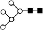
1580		Man a1-3 (Man a1-3 (Man a1-6) Man a1-6) Man b1-4 GlcNAc b1-4 GlcNAc	1579.7834	1235.1172	carbNlink_2 0482_D000	beta-glucuronidase 35, cytochrome P450 36, apolipoprotein B-100 42, IgM 43, Interleukin 6 44
2040‡		GlcNAc b1-2 Man a1-3 (Gal bl- 4 GlcNAc b1-2 Man a1-6) Man b1- 4 GlcNAc b1-4 (Fuc a1-6) GlcNAc or GlcNAc b 1-4 Man a1-3 (Gal bl- 4 GlcNAc bl-2 Man a1-6) Man b1- 4 GlcNAc b1-4 (Fuc a1-6) GlcNAc	2040.0254	1641.5072	carbNlink_2 1240_D000	IgG38,39,45
2187‡		NeuAc a2-3 Gal b1-4 GlcNAc bl-2 Man a1-3 (Man a1-3 Man a1- 6) Man b1-4 GlcNAc b1-4 GlcNAc	2186.0834	1729.55	carbNlink_4 3948_D000	human chorionic gonadotrophin 37
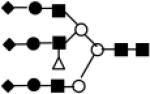
2851		GlcNAc b1-4 (NeuAc a2-6 Gal b1- 4GlcNAc b1-2 Man a1-3) (Gal b1- 4 GlcNAc b1-2 Man a1-6) Man b1- 4 GlcNac b1-4 (Fuc a1-6) GlcNAc or GlcNAc b1-4 (Gal b1-4 GlcNAc b1- 2 Man a1-3) (NeuAc a2-6 Gal b1- 4 GlcNAc b1-2 Man a1-6) Man b1- GlcNAc4 GlcNAc b1-4 (Fuc a1-6) GlcNAc	2850.4252	2282.09	carbNlink_4 1422_D000	IgGl40,41
4502*‡		NeuAc a2-6=2%| NeuAc a2-6=1%| 2% 1% NeuAc a2-6 Gal b1- 4 GlcNac b1-2 (2% 1% NeuAc a2- 6 Gal b1-4 (Fuc a1-3) GlcNAc b1-4) Man a1-3/6 (2% 1% NeuAc a2-6 Gal b1-4 GlcNAc b1-2 Man a1-6/3) Man b1-4 GlcNAc b1-4 GlcNAC	4500	3625.2761	carbNlink_2 1379_P	CD45 (PTPRC protein tyrosine phosphatase, receptor type, C)46

^†Symbol for representation of Sugar type ■ GlcNAc; ○ Man; ● Gal; △ Fuc; ◆ NeuAc.

^*Structural analysis of this glycan is underway. According to the molecular weight and isotopic distribution of this glycan, we found this possible match by searching through glycan database.

⁺The information was obtained from glycan database Web site: http://www.functionalglycomics.org/glycomics/molecule/jsp/carbohydrate/carbMoleculeHome.jsp

^‡These peaks were identified in our previous study.¹⁴,¹⁸-²⁰

Literature search indicates that some cancer-related proteins have glycan compositions as the four glycans we selected with known structure. The high mannose glycan at MW 1580 could be enzymatically released from a research anticancer target beta-glucuronidase (hCG)^34,35 and a successful anticancer target cytochrome P450.^34,36 Glycan at MW 2187 could be released from a research anticancer target chorionic gonadotrophin.^34,37 The expressions of these two glycans were gradually increased from healthy people, CLD to HCC cases (Figure 3), implicating possibly important involvement of these two glycans and their associated glycoproteins in the HCC progression. The two fucosylated glycans at MW 2040 and 2851 could be enzymatically released from human immunoglobulin IgG.^38-41 A comprehensive determination of the glycan composition at glycosylation sites in these proteins is needed to reveal post-translational modifications of glycoprotein, analyze specific function to the carbohydrate moiety, and determine the potential clinical utility of the glycan markers for early diagnosis of HCC.

4. Conclusion

Changes in glycosylation are associated with physiological and pathophysiological conditions of cells. Glycan marker discovery would be helpful to determine the physiological state of patients. We identified 7 N-glycan serum markers associated with HCC from mass spectrometry data. We used the 7 glycans to achieve good performance in distinguishing HCC patients from CLD patients and healthy people with unsupervised clustering and supervised classification methods and with newly generated data set. The structures of 4 glycans could be identified in the important cancer-related glycoproteins. Further analysis and evaluation of these marker candidates are needed to validate their clinical utility for early diagnosis of HCC.

References

- 1.Walsh G, Jefferis R. Post-translational modifications in the context of therapeutic proteins. Nat. Biotechnol. 2006;24(10):1241–52. doi: 10.1038/nbt1252. [DOI] [PubMed] [Google Scholar]
- 2.Fuster MM, Esko JD. The sweet and sour of cancer: glycans as novel therapeutic targets. Nat. Rev. Cancer. 2005;5(7):526–42. doi: 10.1038/nrc1649. [DOI] [PubMed] [Google Scholar]
- 3.Dube DH, Bertozzi CR. Glycans in cancer and inflammation--potential for therapeutics and diagnostics. Nat. Rev. Drug Discovery. 2005;4(6):477–88. doi: 10.1038/nrd1751. [DOI] [PubMed] [Google Scholar]
- 4.Kobata A, Amano J. Altered glycosylation of proteins produced by malignant cells, and application for the diagnosis and immunotherapy of tumours. Immunol. Cell Biol. 2005;83(4):429–39. doi: 10.1111/j.1440-1711.2005.01351.x. [DOI] [PubMed] [Google Scholar]
- 5.Macdonald JS. Carcinoembryonic antigen screening: pros and cons. Semin. Oncol. 1999;26(5):556–60. [PubMed] [Google Scholar]
- 6.Kui Wong N, Easton RL, Panico M, Sutton-Smith M, Morrison JC, Lattanzio FA, Morris HR, Clark GF, Dell A, Patankar MS. Characterization of the oligosaccharides associated with the human ovarian tumor marker CA125. J. Biol. Chem. 2003;278(31):28619–34. doi: 10.1074/jbc.M302741200. [DOI] [PubMed] [Google Scholar]
- 7.Basu PS, Majhi R, Batabyal SK. Lectin and serum-PSA interaction as a screening test for prostate cancer. Clin. Biochem. 2003;36(5):373–6. doi: 10.1016/s0009-9120(03)00050-x. [DOI] [PubMed] [Google Scholar]
- 8.Peracaula R, Tabares G, Royle L, Harvey DJ, Dwek RA, Rudd PM, de Llorens R. Altered glycosylation pattern allows the distinction between prostate-specific antigen (PSA) from normal and tumor origins. Glycobiology. 2003;13(6):457–70. doi: 10.1093/glycob/cwg041. [DOI] [PubMed] [Google Scholar]
- 9.Meany DL, Zhang Z, Sokoll LJ, Zhang H, Chan DW. Glycoproteomics for Prostate Cancer Detection: Changes in Serum PSA Glycosylation Patterns. J. Proteome Res. 2009;8(2):613–9. doi: 10.1021/pr8007539. [DOI] [PMC free article] [PubMed] [Google Scholar]
- 10.Greten TF, Papendorf F, Bleck JS, Kirchhoff T, Wohlberedt T, Kubicka S, Klempnauer J, Galanski M, Manns MP. Survival rate in patients with hepatocellular carcinoma: a retrospective analysis of 389 patients. Br. J. Cancer. 2005;92(10):1862–8. doi: 10.1038/sj.bjc.6602590. [DOI] [PMC free article] [PubMed] [Google Scholar]
- 11.Filmus J, Capurro M. Glypican-3 and alphafetoprotein as diagnostic tests for hepatocellular carcinoma. Mol. Diagn. 2004;8(4):207–12. doi: 10.1007/BF03260065. [DOI] [PubMed] [Google Scholar]
- 12.Yu J, Chen XW. Bayesian neural network approaches to ovarian cancer identification from high-resolution mass spectrometry data. Bioinformatics. 2005;21(Suppl 1):i487–94. doi: 10.1093/bioinformatics/bti1030. [DOI] [PubMed] [Google Scholar]
- 13.Herbst A, McIlwain S, Schmidt JJ, Aiken JM, Page CD, Li L. Prion disease diagnosis by proteomic profiling. J. Proteome Res. 2009;8(2):1030–6. doi: 10.1021/pr800832s. [DOI] [PMC free article] [PubMed] [Google Scholar]
- 14.Ressom HW, Varghese RS, Goldman L, An Y, Loffredo CA, Abdel-Hamid M, Kyselova Z, Mechref Y, Novotny M, Drake SK, Goldman R. Analysis of MALDI-TOF mass spectrometry data for discovery of peptide and glycan biomarkers of hepatocellular carcinoma. J. Proteome Res. 2008;7(2):603–10. doi: 10.1021/pr0705237. [DOI] [PMC free article] [PubMed] [Google Scholar]
- 15.Wu B, Abbott T, Fishman D, McMurray W, Mor G, Stone K, Ward D, Williams K, Zhao H. Comparison of statistical methods for classification of ovarian cancer using mass spectrometry data. Bioinformatics. 2003;19(13):1636–43. doi: 10.1093/bioinformatics/btg210. [DOI] [PubMed] [Google Scholar]
- 16.Tang ZQ, Han LY, Lin HH, Cui J, Jia J, Low BC, Li BW, Chen YZ. Derivation of stable microarray cancer-differentiating signatures using consensus scoring of multiple random sampling and gene-ranking consistency evaluation. Cancer Res. 2007;67(20):9996–10003. doi: 10.1158/0008-5472.CAN-07-1601. [DOI] [PubMed] [Google Scholar]
- 17.Mahadevan S, Shah SL, Marrie TJ, Slupsky CM. Analysis of metabolomic data using support vector machines. Anal. Chem. 2008;80(19):7562–70. doi: 10.1021/ac800954c. [DOI] [PubMed] [Google Scholar]
- 18.Goldman R, Ressom HW, Varghese RS, Goldman L, Bascug G, Loffredo CA, Abdel-Hamid M, Gouda I, Ezzat S, Kyselova Z, Mechref Y, Novotny MV. Detection of hepatocellular carcinoma using glycomic analysis. Clin. Cancer Res. 2009;15(5):1808–13. doi: 10.1158/1078-0432.CCR-07-5261. [DOI] [PMC free article] [PubMed] [Google Scholar]
- 19.Varghese RS, Goldman L, An Y, Loffredo CA, Abdel-Hamid M, Kyselova Z, Mechref Y, Novotny M, Drake SK, Goldman R, Ressom HW. Integrated peptide and glycan biomarker discovery using MALDI-TOF mass spectrometry. Conf. Proc. IEEE Eng. Med. Biol. Soc. 2008;2008:3791–4. doi: 10.1109/IEMBS.2008.4650034. [DOI] [PMC free article] [PubMed] [Google Scholar]
- 20.Ressom HW, Varghese RS, Goldman L, Loffredo CA, Abdel-Hamid M, Kyselova Z, Mechref Y, Novotny M, Goldman R. Analysis of MALDI-TOF mass spectrometry data for detection of glycan biomarkers. Pac. Symp. Biocomput. 2008:216–27. [PMC free article] [PubMed] [Google Scholar]
- 21.Goldman R, Ressom HW, Abdel-Hamid M, Goldman L, Wang A, Varghese RS, An Y, Loffredo CA, Drake SK, Eissa SA, Gouda I, Ezzat S, Moiseiwitsch FS. Candidate markers for the detection of hepatocellular carcinoma in low-molecular weight fraction of serum. Carcinogenesis. 2007;28(10):2149–53. doi: 10.1093/carcin/bgm177. [DOI] [PMC free article] [PubMed] [Google Scholar]
- 22.Novotny MV, Mechref Y. New hyphenated methodologies in high-sensitivity glycoprotein analysis. J. Sep. Sci. 2005;28(15):1956–68. doi: 10.1002/jssc.200500258. [DOI] [PMC free article] [PubMed] [Google Scholar]
- 23.Mechref Y, Novotny MV. Miniaturized separation techniques in glycomic investigations. J. Chromatogr. B, Anal. Technol. Biomed. Life Sci. 2006;841(1–2):65–78. doi: 10.1016/j.jchromb.2006.04.049. [DOI] [PubMed] [Google Scholar]
- 24.Coombes KR, Tsavachidis S, Morris JS, Baggerly KA, Hung MC, Kuerer HM. Improved peak detection and quantification of mass spectrometry data acquired from surface-enhanced laser desorption and ionization by denoising spectra with the undecimated discrete wavelet transform. Proteomics. 2005;5(16):4107–17. doi: 10.1002/pmic.200401261. [DOI] [PubMed] [Google Scholar]
- 25.Jeffries N. Algorithms for alignment of mass spectrometry proteomic data. Bioinformatics. 2005;21(14):3066–73. doi: 10.1093/bioinformatics/bti482. [DOI] [PubMed] [Google Scholar]
- 26.Vapnik V. Statistical Learning Theory. Wiley; New York: 1998. [Google Scholar]
- 27.Ressom HW, Varghese RS, Drake SK, Hortin GL, Abdel-Hamid M, Loffredo CA, Goldman R. Peak selection from MALDI-TOF mass spectra using ant colony optimization. Bioinformatics. 2007;23(5):619–26. doi: 10.1093/bioinformatics/btl678. [DOI] [PubMed] [Google Scholar]
- 28.Ressom HW, Varghese RS, Abdel-Hamid M, Eissa SA, Saha D, Goldman L, Petricoin EF, Conrads TP, Veenstra TD, Loffredo CA, Goldman R. Analysis of mass spectral serum profiles for biomarker selection. Bioinformatics. 2005;21(21):4039–45. doi: 10.1093/bioinformatics/bti670. [DOI] [PubMed] [Google Scholar]
- 29.Cui J, Liu Q, Puett D, Xu Y. Computational prediction of human proteins that can be secreted into the bloodstream. Bioinformatics. 2008;24(20):2370–5. doi: 10.1093/bioinformatics/btn418. [DOI] [PMC free article] [PubMed] [Google Scholar]
- 30.Platt J. Fast Training of Support Vector Machines using Sequential Minimal Optimization. MIT Press; Cambridge, MA: 1998. [Google Scholar]
- 31.Keerthi SS, Lin CJ. Asymptotic behaviors of support vector machines with Gaussian kernel. Neural Comput. 2003;15(7):1667–89. doi: 10.1162/089976603321891855. [DOI] [PubMed] [Google Scholar]
- 32.Eisen MB, Spellman PT, Brown PO, Botstein D. Cluster analysis and display of genome-wide expression patterns. Proc. Natl. Acad. Sci. U.S.A. 1998;95(25):14863–8. doi: 10.1073/pnas.95.25.14863. [DOI] [PMC free article] [PubMed] [Google Scholar]
- 33.Mechref Y, Novotny MV. Mass spectrometric mapping and sequencing of N-linked oligosaccharides derived from submicrogram amounts of glycoproteins. Anal. Chem. 1998;70(3):455–63. doi: 10.1021/ac970947s. [DOI] [PubMed] [Google Scholar]
- 34.Chen X, Ji ZL, Chen YZ. TTD: Therapeutic Target Database. Nucleic Acids Res. 2002;30(1):412–5. doi: 10.1093/nar/30.1.412. [DOI] [PMC free article] [PubMed] [Google Scholar]
- 35.Howard DR, Natowicz M, Baenziger JU. Structural studies of the endoglycosidase H-resistant oligosaccharides present on human beta-glucuronidase. J. Biol. Chem. 1982;257(18):10861–8. [PubMed] [Google Scholar]
- 36.Szczesna-Skorupa E, Kemper B. An N-terminal glycosylation signal on cytochrome P450 is restricted to the endoplasmic reticulum in a luminal orientation. J. Biol. Chem. 1993;268(3):1757–62. [PubMed] [Google Scholar]
- 37.Weisshaar G, Hiyama J, Renwick AG. Site-specific N-glycosylation of human chorionic gonadotrophin--structural analysis of glycopeptides by one- and two-dimensional 1H NMR spectroscopy. Glycobiology. 1991;1(4):393–404. doi: 10.1093/glycob/1.4.393. [DOI] [PubMed] [Google Scholar]
- 38.Harada H, Kamei M, Tokumoto Y, Yui S, Koyama F, Kochibe N, Endo T, Kobata A. Systematic fractionation of oligosaccharides of human immunoglobulin G by serial affinity chromatography on immobilized lectin columns. Anal. Biochem. 1987;164(2):374–81. doi: 10.1016/0003-2697(87)90507-0. [DOI] [PubMed] [Google Scholar]
- 39.Arbatskii NP, Martynova MD, Aleshkin VA, Derevitskaia VA. Structural analysis of carbohydrate chains of normal and myeloma immunoglobulins G using HPLC. Bioorg. Khim. 1989;15(2):175–80. [PubMed] [Google Scholar]
- 40.Savvidou G, Klein M, Grey AA, Dorrington KJ, Carver JP. Possible role for peptide-oligosaccharide interactions in differential oligosaccharide processing at asparagine-107 of the light chain and asparagine-297 of the heavy chain in a monoclonal IgG1 kappa. Biochemistry. 1984;23(16):3736–40. doi: 10.1021/bi00311a026. [DOI] [PubMed] [Google Scholar]
- 41.Ohkura T, Isobe T, Yamashita K, Kobata A. Structures of the carbohydrate moieties of two monoclonal human lambda-type immunoglobulin light chains. Biochemistry. 1985;24(2):503–8. doi: 10.1021/bi00323a038. [DOI] [PubMed] [Google Scholar]
- 42.Taniguchi T, Ishikawa Y, Tsunemitsu M, Fukuzaki H. The structures of the asparagine-linked sugar chains of human apolipoprotein B-100. Arch. Biochem. Biophys. 1989;273(1):197–205. doi: 10.1016/0003-9861(89)90179-3. [DOI] [PubMed] [Google Scholar]
- 43.Cahour A, Debeire P, Hartmann L, Montreuil J. Comparative study of the carbohydrate moieties of normal and pathological human immunoglobulins M. Biochem. J. 1983;211(1):55–63. doi: 10.1042/bj2110055. [DOI] [PMC free article] [PubMed] [Google Scholar]
- 44.Parekh RB, Dwek RA, Rademacher TW, Opdenakker G, Van Damme J. Glycosylation of interleukin-6 purified from normal human blood mononuclear cells. Eur. J. Biochem. 1992;203(1–2):135–41. doi: 10.1111/j.1432-1033.1992.tb19838.x. [DOI] [PubMed] [Google Scholar]
- 45.Patel TP, Parekh RB, Moellering BJ, Prior CP. Different culture methods lead to differences in glycosylation of a murine IgG monoclonal antibody. Biochem. J. 1992;285(Pt 3):839–45. doi: 10.1042/bj2850839. [DOI] [PMC free article] [PubMed] [Google Scholar]
- 46.Sato T, Furukawa K, Autero M, Gahmberg CG, Kobata A. Structural study of the sugar chains of human leukocyte common antigen CD45. Biochemistry. 1993;32(47):12694–704. doi: 10.1021/bi00210a019. [DOI] [PubMed] [Google Scholar]