Eye movement statistics in humans are consistent with an optimal search strategy

Abstract

Most models of visual search are based on the intuition that humans choose fixation locations containing features that best match the features of the target. The optimal version of this feature-based strategy is what we term “maximum a posteriori (MAP) search.” Alternatively, humans could choose fixations that maximize information gained about the target's location. We term this information-based strategy “ideal search.” Here we compare eye movements of human, MAP, and ideal searchers in tasks where known targets are embedded at unknown locations within random backgrounds having the spectral characteristics of natural scenes. We find that both human and ideal searchers preferentially fixate locations in a donut-shaped region around the center of the circular search area, with a high density of fixations at top and bottom, while MAP searchers distribute their fixations more uniformly, with low density at top and bottom. Our results argue for a sophisticated search mechanism that maximizes the information collected across fixations.

Introduction

Few tasks are more important for survival than visually searching the local environment for relevant objects. In performing visual search under natural conditions, humans use high-speed eye movements (saccades) to direct the highest resolution region of the retina, the fovea, toward potential target locations in the environment. Despite decades of research, relatively little is known about how humans actually select fixation locations in visual search, although a number of computational models have been proposed (Findlay, 1997; Findlay & Walker, 1999; Itti & Koch, 2000; Itti, Koch, & Niebur, 1998; Koch & Ullman, 1985; Najemnik & Geisler, 2005; Olshausen, Anderson, & Van Essen, 1993; Peters, Iyer, Itti, & Koch, 2005; Rao, Zelinsky, Hayhoe, & Ballard, 2002; Treisman, 1988; Wolfe, 1994).

Conceptually, the processing involved in visual search tasks can be described within the general probabilistic framework depicted by the flowchart in Figure 1. A searcher starts with some initial prior beliefs about the potential locations of the target. These beliefs might be represented as prior probabilities of the target being located at every potential location in the visual scene. During the first fixation, the searcher captures visual data from the retinal image and uses that data to update its beliefs about the target location. These updated beliefs might be represented as posterior probabilities. If the posterior probability at some location gets large enough, then the search is stopped, and the location with the largest posterior probability is picked as the target location. (In search tasks where the target can be absent, the search can also stop if the posterior probability of no target gets large enough.) If the stopping criterion is not exceeded, then the searcher chooses the next location to fixate and the process repeats until the searcher finds the target. Thus, within this framework, visual search tasks present three challenges for the searcher: encoding visual information on each fixation, integrating information across fixations, and selecting successive fixation locations.

Figure 1.

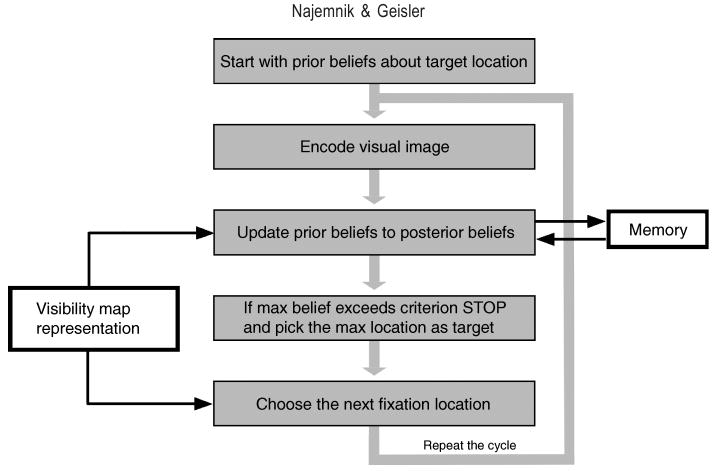
Visual search in a probabilistic framework. The searcher starts with some initial prior beliefs (represented as probabilities) about the target being located at every potential location in the visual scene. During the first fixation, the searcher encodes visual data from all the potential target locations and uses it to update its prior beliefs to posterior beliefs. If the posterior probability at some location exceeds a criterion, then the search is stopped and the location with the largest posterior probability is picked as the target location. If the criterion is not exceeded, the searcher chooses the next location to fixate, and the process repeats until the searcher finds the target. The searcher's representation of its own visual limitations (i.e., the detectability of the target across the visual field) can affect how it updates its beliefs and how it chooses the next fixation location. The searcher's memory limitations can affect the beliefs stored across fixations. An ideal searcher that aims to find the target quickly (i) has perfect memory, (ii) has precise knowledge about the target, about the statistical properties of the visual scene in which the target is embedded, and about its own visual system, and (iii) makes the eye movements that that on average will gain the most information about the target's location.

A Bayesian ideal searcher that aims to find the target quickly will capture image data in parallel from every possible target location, will integrate the information perfectly within and across fixations, and will make the eye movements that gain the most information about the target's location (maximize the accuracy of localizing the target). An optimally efficient MAP searcher will do everything the same as the ideal searcher, except it will make eye movements to the most likely target location (the location with the currently greatest posterior probability), which is not necessarily a location that will result in maximum information gain. Recently, we (Najemnik & Geisler, 2005) derived the algorithm for the Bayesian ideal searcher, simulated its performance given the same constraint on target detectability across its retina as the human visual system, and found that human searchers achieve near-optimal performance (as measured by the numbers of fixations and error rate) when searching for small targets in backgrounds of 1/f noise, which have Fourier amplitude spectra similar to natural images (see the target and background texture in Figure 2A). We also showed that to achieve this nearly ideal performance in our task humans must have sufficient memory for past fixation locations to reduce the probability of revisiting them and must perform efficient parallel detection on each fixation (for additional evidence of efficient parallel detection, see Eckstein, Beutter, & Stone, 2001; Eckstein, Thomas, Palmer, & Shimozaki, 2000; Palmer, Verghese, & Pavel, 2000).

Figure 2.

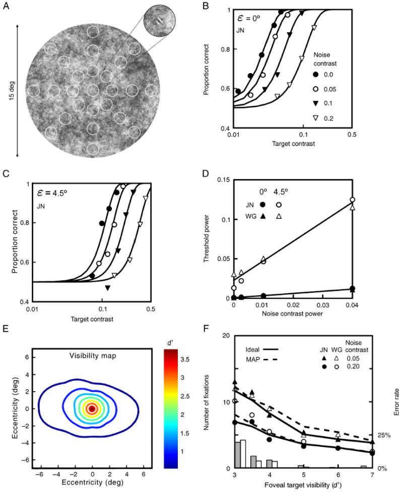
Target visibility maps and search performance. (A) To measure visibility maps, psychometric functions (detection accuracy as a function of target contrast) were measured at the twenty-five locations indicated by the circles (the circles did not appear in the display). (B) Proportion of correct responses in the fovea, as a function of target rms contrast, for four levels of background noise rms contrast (from Najemnik & Geisler, 2005). (C) Proportion of correct responses at 4.5 deg eccentricity, as a function of target contrast, for the same four levels of background contrast. (D) Detection threshold contrast power (the square of rms contrast) of the target as a function of noise contrast power in the fovea and at 4.5 degrees eccentricity, for two observers. The detection threshold is defined to be the contrast power of the target corresponding to 82% correct. (E) Contour plot of the visibility map (d′ as a function of retinal position) for one combination of target and background contrast, based on the average psychometric-function data from the two observers. Note that the signal-to-noise ratio d′ is monotonically related to the probability of a correct response in the detection task (see Methods). (F) Median number of fixations on correct search trials, as a function of target detectability at the center of the fovea, for two human searchers (symbols), the ideal searcher (solid curves) and the MAP searcher (dashed curves). (The data points and solid curves are from Najemnik & Geisler, 2005.) The histograms show the error rates for the human searchers (gray) and the ideal searcher (white)

Most models of visual search assume that humans compute feature maps of some sort and then direct fixations to the locations within the visual scene where the features are most similar to the target (Findlay, 1997; Findlay & Walker, 1999; Itti & Koch, 2000; Itti et al., 1998; Koch & Ullman, 1985; Olshausen et al., 1993; Peters, et al., 2005; Rao et al., 2002; Treisman, 1988; Wolfe, 1994). In the context of the probabilistic framework in Figure 1, this strategy corresponds most closely to MAP search; i.e., fixating the location with the greatest likelihood of being the location of the target, given the features collected on previous fixations (however, for a more sophisticated strategy of fixation selection, see Rao et al., 2002). Thus, the MAP searcher can be regarded as an optimal form of feature-based searcher when the task is to find a specific target. As shown later, a MAP searcher can achieve search performance similar to human searchers (and only a little poorer than ideal), and thus it is a plausible model of human fixation selection on the grounds of overall performance. However, the MAP fixation selection strategy differs markedly from the ideal. The ideal searcher not only makes MAP-like fixations, but “center-of-gravity” fixations, “exclusion” fixations, and other hard to classify fixations, all with the goal of maximizing the information collected on each fixation (Najemnik & Geisler, 2005). Here we ask whether humans in a naturalistic search task are better modeled as a MAP (feature-based) searcher or as something closer to an ideal (information-based) searcher. To answer this question, we compare how human, ideal, and MAP searchers distribute their fixations across the search area. Importantly, the fixation distribution of a searcher depends critically on how the detectability (visibility) of the target varies as function of retinal location. Thus, we start by determining the full 2D human visibility map from our detection measurements (Najemnik & Geisler, 2005) and then constrain the two model searchers with the same map. For simplicity, our previous paper reported the visibility map averaged across direction from the fovea because the averaging had only a small effect on the predicted ideal search time and error rate. Here, however, we show that the full visibility map has significant anisotropies, and that these anisotropies affect, in different ways, the fixation distributions predicted by the ideal and MAP searchers.

Methods

In our search task, the target was a small sine wave pattern randomly located at one of 85 target locations densely covering a circular 1/f noise background region 15 deg in diameter. An example of the noise background with an added target is shown in Figure 2A (the 25 circles indicate target locations for a separate target detection experiment; see below). The observer was required to press a button as soon as the target was located and then to indicate the location by fixating the target and pressing the button again; the trial was counted as correct if the eye was closer to the true target location than any other potential target location. The observer's eye position was continuously monitored with a high-precision eye tracker. The first step in evaluating models for this search task is to measure detection sensitivity across the visual field (visibility maps) for the stimulus conditions under which the search performance was measured. To determine the visibility maps, detection accuracy as a function of target contrast (a psychometric function) was measured at each of the 25 locations indicated by the circles in Figure 2A, for four different levels of noise contrast (see Najemnik & Geisler, 2005).

Observers

The observers were the two authors. Both were experienced psychophysical observers with normal or corrected-to-normal acuity and were naive about the predictions of the ideal and MAP searchers at the time the search data were collected. Also, a third completely naive observer produced similar overall search performance in a very similar search experiment, although visibility maps were not measured for that observer (Geisler, Perry, & Najemnik, 2006).

Stimuli and apparatus

The stimuli were displayed on a calibrated monochrome IMAGE SYSTEMS monitor (M21L) with white phosphor (P-104) at a frame rate of 60 Hz. The monitor displayed 1024 × 768 pixels, which subtended a visual angle of 20.6 × 15.4 degrees from the viewing distance of 112 cm. The red, green, and blue signals from a Matrox Dual Head graphics card were combined into one voltage that drove the monitor gun, allowing for a fine control of the contrast displayed on the screen (Pelli & Zhang, 1991). The target was a 6 cycle per degree (cpd) sine wave grating, tilted 45 deg to the left, and windowed by a symmetric raised cosine (half-height width one cycle). The background was a circular region 15 deg in diameter, filled with 1/f noise at a mean luminance of 40 cd/m²; the display outside the background region was set to the mean luminance. The 1/f noise was created by filtering Gaussian white noise in the Fourier domain, truncating the filtered noise waveform to ± 2 SD (0.46% of the noise pixels clipped), scaling to obtain the desired RMS amplitude, and then adding a constant to obtain the mean luminance. Eye position was measured with a Forward-Technologies SRI Version-6 dual Purkinje eye tracker. The eye-position signals were sampled from the eye tracker at 100 Hz by a National Instruments data acquisition board. Head position was maintained with a bite bar and headrest. To calibrate the eye tracker, the observer was asked to fixate points on a 3 × 3 calibration grid, and the results were then used to establish the transformation between the output voltages of the eye tracker and the position of the observer's gaze on the computer display. The algorithm for computing fixation points from eye positions was a modified version of one in the Applied Science Laboratory Series 5000 data analysis software.

The retinal map of target detectability

To characterize the retinal map of target detectability (the visibility map) for each of the conditions in the search experiment described below, detection accuracy was measured for the 6 cpd sine wave target as function of target contrast and the contrast of the background noise, at the 25 spatial locations indicated by the small circles in Figure 2A. The observer was required to fixate the center of the display, which was monitored with an eye tracker, and for each block of trials, the target was presented at only a single known location. The experiment was divided into 40-minute sessions. Each session was devoted to measuring the psychometric function for detecting the target at one of the 25 retinal locations, in four levels of external noise, and consisted of 16 blocks of 32 trials. The trials in the session were blocked by target contrast (4 contrast levels per psychometric function, as determined in pilot sessions), and noise rms contrast (0.00, 0.05, 0.10, 0.20), where rms contrast is defined as the standard deviation of the pixel luminance divided by the mean luminance. Each block was preceded by a foveal presentation of the target alone in order to re-familiarize the observer with the target. The trial started when the observer fixated the fixation spot (to prevent masking there was no fixation dot for the foveal measurements) at the centre of the screen, and pressed a button. In 0.75 s the fixation spot disappeared, and the first stimulus interval was presented for 0.25 s, followed by a blank screen with a fixation spot for 0.5 s, followed by the second stimulus interval (0.25 s), followed by a blank screen with a fixation spot until the response was made. One stimulus interval contained background noise alone, the other a different random sample of background noise with the target added. The observer judged which stimulus interval contained the target by pressing one of two buttons on a button box. After the response was made, a cue (an 0.45 deg cross with rms contrast 0.4) appeared at the target location and stayed there for 0.75 s. The cross served to remind the observer of the target location after each trial. We chose to present this cue after the response was made rather than before each trial in order to avoid stimulus masking. The observer's fixation location was monitored throughout, and a warning signal was sounded after each trial where the observer was not fixated within 0.75 deg of the fixation spot throughout the presentation of the test stimuli. These trials were discarded. The eye tracker calibration was repeated before each block, and the observer had the option to recalibrate after each trial by pressing a recalibration button. The detection data measured at each location, for each contrast and for each observer, were fit with a modified Weibull function:

$$f(c)=0.5+0.5(1-\text{exp}{[-c/c_T)}^s]),$$ (1)

where c_T is a position parameter and s is a steepness parameter. We interpolated the psychometric functions measured at the 25 locations to obtain a continuous map of human detection accuracy across the visual field. Specifically, we interpolated the psychometric functions, using a surface interpolation technique that assumes the interpolant is the sum of 25 radial linear basis functions centered on the 25 locations where we made measurements (Carr, Fright, & Beatson, 1997). This visibility map was then used to constrain the ideal and MAP search models.

Human visual search

On each trial of the search task, the observer first fixated a dot at the center of the display and then initiated the trial with a button press. The fixation dot disappeared immediately and a random time later (100–500 ms) the search display appeared. The target was randomly embedded in a background of 1/f noise at one of 85 locations densely tiling the 15 deg display in a triangular array. The observer's task was to find the target as rapidly as possible without making errors. As soon as the target was located, the observer pressed a button, a little dot was rendered at the observer's point of gaze in real time. The observer then indicated the judged location of the target by fixating that location and pressing the button again. The response was considered correct if the eye position (at the time of the second button press) was closer to the target location than to any other potential target location. Prior to each block, the eye tracker was calibrated and the search target was shown on a uniform background at the center of the display. Each observer completed at least twelve 40-minute sessions. Each session consisted of 6 blocks of 32 search trials. The trials in the session were blocked by target contrast (six contrast levels per session). The rms contrast of the background noise was fixed within each session. The six target contrast levels were set based on the results of the detection experiment described above so that they corresponded to six levels of foveal detectability d′ = 3, 3.5, 4, 5, 6, and 7 (d′ is monotonically related to detection accuracy; see later for more details). Two contrast levels for the background noise were tested, 0.05 and 0.20 rms. The eye-tracker calibration was repeated prior to each block. The observer had an option to recalibrate after each trial by pressing a recalibration button.

Simulation of ideal and MAP searchers

The eye movements of both the ideal and MAP searchers depend critically on how the detectability of the target varies across the visual field. For example, if this visibility maps were uniform, then the ideal strategy is not to move the eyes at all. We constrained the ideal and MAP searchers with the human visibility map. Our explicit model of human target detection is based on signal detection theory, which describes detection as noisy template matching. The detector multiplies the retinal image with a template of the sine wave target and then integrates the product to obtain a template response (i.e., the template response is the spatial correlation of the target with the retinal stimulus). The magnitude of this template response is then compared to a criterion; the optimal behavior is to respond “target present” if the template response exceeds a criterion and “target absent” otherwise. In addition to noise in the physical stimulus, the template response is further assumed to be corrupted by “internal noise” that accounts for the detector's own inefficiencies. The performance of this detector, when limited by both external and internal noise, can be represented by a signal-to-noise ratio d′(p; c, e_n), where p is the retinal position, c is the rms contrast of the target, and e_n is the contrast power (rms contrast squared) of the background noise. The signal-to-noise ratio is monotonically related to detection accuracy and is obtained by taking the inverse normal integral of the accuracy function, f(p; c, e_n), measured in the visibility-map experiment

$$d\text{'}(\mathbf{\text{p}};c,e_n)=\sqrt{2}{\Phi }^{-1}[f(\mathbf{\text{p}};c,e_n)],$$ (2)

where Φ⁻[x] is the inverse of the standard normal integral. The √2 factor takes into account that there were two intervals in the forced choice detection task described above, but (effectively) only a single interval in each fixation of the search task (Green & Swets, 1966). In the auxiliary material we show that

$$d\text{'}{(\mathbf{\text{p}};c,e_n)}^2=\frac{c^2}{\alpha e_n+\beta (\mathbf{\text{p}};c,e_n)},$$ (3)

where αe_n is the effective 1/f noise power passing through the sine wave template and β(p; c, e_n) is the effective noise from the observer's own sources of inefficiency, which might include internal variability, reduced spatial resolution in the periphery, criterion variations, and so on (Burgess & Ghandeharian, 1984; Lu & Dosher, 1999; Pelli & Farell, 1999). The value of α(= 0.0218) was determined by measuring the template responses to the target and by measuring the variance of the template responses to very large number of samples of the actual background noise used in the experiments. Once α was determined, the values of β(p; c, e_n) were obtained directly from the psychophysically measured visibility map using Equations 2 and 3. We also note that the signal-to-noise ratio for an ideal detector limited only by external noise is given by $d_E^{\prime }{(c,e_n)}^2=c^2/\alpha e_n$ and the signal-to-noise ratio of an ideal detector limited by only by the internal inefficiencies is given by $d_I^{\prime }{(\mathbf{\text{p}};c,e_n)}^2=c^2/\beta {(\mathbf{\text{p}};c,e_n)}^2$.

To describe the steps of the simulations, let W_ik(t) be the template response from potential target location i on the t^th fixation, where the fixation location is k(t). Similarly, let $d_I^{\prime }[i,k(t)]$ and $d_E^{\prime }$ be the corresponding signal-to-noise ratios. Here we have simplified the notation by dropping c and e_n. The retinal position p is given implicitly by the values of i and k(t). The steps for each simulated search trial were implemented as follows:

1. Fixation began at the center of the display (as in the search experiment).

2. One of the n possible target locations was selected at random (prior(i) = 1/n); 0.5 was added to that location and −0.5 to all other locations. This gives the template responses an expected value of 0.5 when the target is at that location and −0.5 otherwise. This was done for mathematical convenience, it has no effect on the predictions as long as we add noise to the simulated template responses so that the values of d′ exactly match those given by the visibility map.

3. A static Gaussian noise sample X_i was generated for each potential target location. These samples were statistically independent with mean zero and variance $1/d_E^{\prime 2}$. Note that these numbers represent the template responses to the external 1/f noise, not the external noise itself. The static noise samples remained the same throughout the search trial, reflecting the fact that the 1/f noise was static.

4. On each fixation t, an independent Gaussian noise sample N_ik(t) was generated for each potential target location and added to the static noise sample. These noise samples had mean zero and variance $1/d_I^{\prime }{[i,k(t)]}^2$. Thus, at the target location the template response is W_ik(t) = X_i + N_ik(t) + 0.5, and at all other locations W_jk(t) = X_j + N_jk(t) − 0.5.

5. The posterior probability at each potential target location i after T fixations was computed using the formula

   $$p_i(T)=\frac{\text{prior}(i)\text{exp}\left[\text{∑}_{t=1}^T{g}_T[i,k(t)]W_{ik(t)}\right]}{\text{∑}_{j=1}^n\text{prior}(j)\text{exp}\left[\text{∑}_{t=1}^T{g}_T[j,k(t)]W_{jk(t)}\right]}$$ (4)

   Where

   $$g_T[i,k(t)]=\frac{d_E^{\prime 2}{d}_I^{\prime }{[i,k(t)]}^2}{d_E^{\prime 2}+\text{∑}_{x=1}^T{d}_I^{\prime }{[i,k(x)]}^2}.$$ (5)

   In other words, optimal integration of information across fixations is achieved by keeping an appropriately weighted sum of the template responses from each potential target location (the sums over t in Equation 4), where the weights, g_T[i, k(t)], are determined by the visibility map. For a derivation, see the auxiliary material. (The icon for this article at the JOV Web site illustrates how the posterior probabilities are updated across fixations.)

6. If the maximum posterior probability exceeded a criterion, the search stopped. The stopping criterion for each condition was picked so that the error rate of the ideal searcher approximately matched that of the human observers (this was done by trial and error).

7. To compute the optimal next fixation point, k_opt(T + 1), the ideal searcher considers each possible next fixation and picks the location that, given its knowledge of the data from previous fixations and the visibility map, will maximize the probability of correctly identifying the location of the target after the next fixation:

   $$k_{\text{opt}}(T+1)=arg\underset{k(T+1)}{max}\left\{\text{∑}_{i=1}^n{p}_i(T)p[C\mid i,k(T)+1)]\right\}.$$ (6)

   Explicit expressions that allow Equation 6 to be evaluated efficiently in simulations are derived in the auxiliary material. The MAP searcher always fixates the location with maximum posterior probability

   $$k_{\text{MAP}}(T+1)=arg\underset{i}{max}[p_i(T)].$$ (7)

8. The process jumps back to step 4 and repeats until the criterion posterior probability is exceeded at some location.

There are several caveats to mention. First, the formal assumption of template matching for target detection affects the search predictions, but the effect is minor. If the external and internal noise are both dynamic (statistically independent), then the specific mechanism of target detection has no effect. In this case, the only thing that matters is the d′ values, which are determined in the preliminary experiment. If the external noise is static (as in the current experiment), then the mechanism of target detection affects the predictions of search performance because it affects the estimated ratio of external to internal noise. However, the effect is small. For example, predicted search performance for the purely dynamic noise case is parallel to and only modestly superior to that predicted for the static external noise case reported here.

Second, the ideal searcher is not really the full ideal because it only considers one fixation into the future (Equation 6). It is not possible to look much further into the future because of the combinatorial explosion of possible fixation sequences. However, we have been able to evaluate the searcher that looks two fixations into the future for one condition and found that ideal performance improved only slightly, considerably less than stepping up from the MAP (which looks ahead zero fixations) to the current ideal (which looks ahead one fixation). Furthermore, we expect little gain from looking far into the future because the posterior probabilities change (with considerable randomness) following each new fixation. Thus, the ideal searcher predictions presented here should be quite close to the full ideal.

Third, the implicit utility (gain/loss) function for the searchers is one that minimizes the number of fixations to find the target while keeping the error rate below a criterion level. As mentioned, we set the criterion level so that the error rate approximately matches human error rate. Once this is done, the predicted search performance and fixation/eye-movement statistics are entirely parameter free.

Finally, we remind the reader that the purpose of deriving and evaluating the ideal searcher is to gain some understanding of what a rational visual system should do (which is not obvious). We do not consider the ideal searcher as plausible model for human search mechanisms. However, it is plausible to suppose that the visual system incorporates heuristic mechanisms that implement some of the rational behaviors of the ideal searcher.

Results

Retinal map of target detectability

The first step in evaluating models for our search task was to measure detection sensitivity across the visual field (visibility maps), for the stimulus conditions under which search performance was measured. To do this, detection accuracy as a function of target contrast (a psychometric function) was measured at each of the 25 locations indicated by the circles in Figure 2A, for four different levels of noise contrast (see Methods).

While maintaining fixation at the center of the display, the observer's task was to indicate which of two temporal intervals contained the target, where the spatial location of the target was known and cued on each trial. Figures 2B and 2C show the measured psychometric functions in the fovea and at one peripheral location, for observer JN. Each psychometric function is for a different rms contrast of the noise background and is summarized with a Weibull function (solid curve), which has a position parameter and a steepness parameter (see Methods). As can be seen, the psychometric functions shift to the right with increasing background noise contrast, and they shift to the right and become steeper with increasing eccentricity. Figure 2D plots the 82% correct contrast thresholds (in units of contrast power—the rms contrast squared) measured in the fovea and at one peripheral location, for both observers. The thresholds fall approximately along straight lines, in agreement with previous studies using white noise backgrounds (Burgess & Ghandeharian, 1984; Lu & Dosher, 1999; Pelli & Farell, 1999). This approximately linear relationship holds for all retinal locations tested, with the slope and intercept varying in a systematic fashion. These systematic relationships (together with the steepness parameter of the psychometric function) can be used to determine by interpolation the target visibility (either the accuracy or the signal-to-noise ratio d′) for any combination of target contrast and background noise contrast, at all possible target locations (see Methods). Figure 2E show how the visibility (d′) of the target varies across the display, for one combination of target contrast and background contrast. The visibility peaks at the center of the fovea and falls off smoothly with retinal eccentricity; it falls fastest in the vertical direction, and thus visibility is poorest in the upper and lower visual fields. There is an anatomical correlate of this asymmetry in the topography of human photoreceptors (Curcio, Sloan, Kalina, & Hendrickson, 1990) and ganglion cells (Curcio & Allen, 1990).

Search performance

Once the visibility maps are specified, it is possible to determine the search behavior predicted by the ideal and MAP searchers. In our earlier study, we found that when the ideal searcher is given the same visibility maps (e.g., Figure 2E) and search error rates as the human searcher, then ideal search performance (median number of fixations) is very similar to human performance (compare symbols and solid curves in Figure 2F; Najemnik & Geisler, 2005). We also found that human efficiency is so high in this search task that most suboptimal models of visual search can be definitively rejected. For example, searchers that fixate randomly, even with perfect memory and perfect integration of information across fixations, perform much poorer than human searchers. The only plausible models remaining are ones that perform near the optimum. A major plausible competitor for the ideal searcher is the feature-based MAP searcher. The dashed curves in Figure 2F show that the performance of the MAP searcher is very similar to human performance and only slightly poorer than that of the ideal searcher (solid curves), and thus cannot be rejected as a model of human search on the basis of overall performance alone. To distinguish between these competing hypotheses for fixation selection, we must turn to eye movement statistics.

Distribution of fixation locations

The density plots in Figures 3A and 3B show that ideal and MAP search strategies make very different predictions for the average spatial distribution of fixation locations across the circular search area, excluding the first fixation at the center of the display. (These plots combine all search trials in all conditions.) The distribution of fixation locations for the ideal searcher has a “donut” shape that peaks at a distance of approximately 5 deg from the center of the display. Furthermore, the ideal distribution of fixation locations has higher density at the top and the bottom of the donut. In other words, the ideal searcher spends more time, on average, at the top and the bottom of the search area. The MAP searcher does not have a donut-shaped distribution of fixation locations and instead covers the search area much more uniformly. (The small donut hole for the MAP searcher is due to excluding the first fixation, which was always in the center of the display.) Also, unlike the ideal, the MAP searcher ventures (on average) further to the left and right sides of the search area. This difference between ideal and MAP fixation statistics can be seen even more clearly by plotting the distributions of fixation direction around the center of the display (red and green curves in Figure 4). In these plots, the ideal and MAP distributions are almost completely out of phase. Finally, note in Figure 3 that the MAP searcher tends to fixate closer to the edge of the display region (dashed circle) than the ideal.

Figure 3.

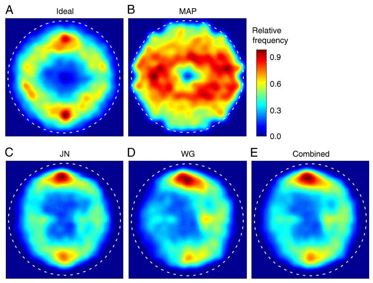
Average spatial distribution of fixation locations across the search area for ideal, map, and human searchers. The color temperature indicates the relative proportion of fixations at each display location. The dashed circles indicate the display region containing the 1/f noise texture. Each of the plots in A through E is based upon approximately 17,000 fixations. The smooth distributions were obtained using a Parzen window with a standard deviation of 0.2 deg.

Figure 4.

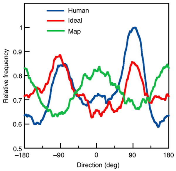
Direction histograms of fixation location relative to the center of the display. The histograms were obtained with a sliding summation window having a width of 45 deg. All three histograms were normalized by the maximum frequency for the human searchers.

Why do the ideal and MAP searchers differ so dramatically in their spatial distribution of fixations? The MAP searcher fixates the most likely location and the most likely location tends to occur in the horizontal direction because the visibility map is elongated in that direction (potential target features are more visible in the horizontal direction). On the other hand, the ideal searcher fixates the location that will provide the most information. Sometimes that location will be near the most likely location, especially when the likelihood is high. However, the ideal searcher implicitly knows that its upper and lower visual fields are less sensitive and hence that often the most information can be gained by shifting gaze into the upper or lower visual fields, especially when the likelihood is not high at any particular location. The ideal also implicitly knows that fixation close to the edge of the display is generally not optimal because it wastes too much of the highly sensitive foveal region. The central finding reported here is that humans have a distribution of fixation locations that is similar to the ideal searcher—a donut-shaped region at a distance of approximately 5 deg from the center, with a higher density of fixations at the top and the bottom (Figures 3C–3E and 4). These results show that humans are more sophisticated than the MAP or similar feature-based searchers, at least in this task. Despite the fact that the authors had no subjective impression of favoring the upper and lower visual fields (and were unaware of the ideal and MAP predictions), they compensated in a rational way for the reduced sensitivity of their eyes in the upper and lower visual fields.

Although human and ideal fixation distributions are similar, there are differences. For example, the human searchers have an initial bias to fixate along the horizontal meridian of the visual field and a later bias to fixate along the vertical meridian, whereas the ideal searcher has initial bias for the vertical meridian and later bias for the horizontal meridian (see Figure A1 in auxiliary material). Initial bias appears to be responsible for some of the asymmetry of the distribution in Figure 3D (see Figure A2 in auxiliary material).

Distribution of saccade vectors

One possible objection to the above account for the distribution of fixation locations is that it could be a result of simple bias in the magnitudes and directions of individual saccades (i.e., preference for making saccades of some lengths and directions over others). But this is not the case. The two-dimensional histograms in Figure 5 show the joint distribution of magnitudes (left axis) and directions (bottom axis) of individual saccades for human, ideal, and MAP searchers.

Figure 5.

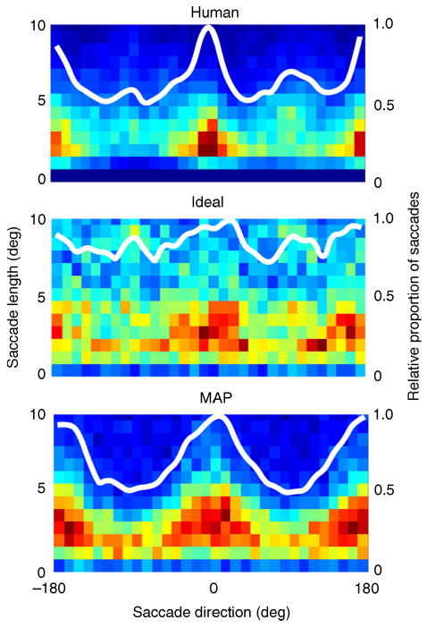
Distribution of saccade vectors for human, ideal, and MAP searchers. In each plot, the saccade take-off point is taken to be the origin, and the color temperature reflects the density of the landing points relative to the origin. In these plots, a rightward saccade has a direction of 0 deg and an upward saccade a direction of 90 deg. The color temperature scale is the same as in Figure 3. The white contours show the relative proportion of saccades in each direction (axis on the right).

All the searchers show a preference for horizontal over vertical saccades; notice the high density of 1°–5° saccades in the horizontal directions (0° and ±180°). Interestingly, a preference for horizontal saccades is exactly the opposite of what might have been expected of a searcher that spends more time at the top and bottom of the search area. Apparently, although humans and ideal searchers spend more time at the top and bottom of the search area, they often use horizontal saccades in getting there. The ideal searcher's tendency to make saccades in the horizontal direction is less pronounced than that of the human and MAP searchers (see white curves and Discussion); however, unlike the MAP searcher, human and ideal searchers have a small secondary peak in the vertical direction (small bumps in the white curves at ±90°), and the saccades tend to be longer in that direction than any other direction (see 2D histograms). We have simulated search strategies that amount to just a random walk across the search area, with the magnitude and direction of each saccade being drawn from the distributions in Figure 5. In all cases, the spatial distribution of fixation locations looks nothing like the ones we actually measured (Figures 3C–3E). Moreover, these kinds of search strategy yield performance far below that of humans and hence can be conclusively rejected.

Discussion

We have considered two classes of models for fixation selection during visual search: ideal search and MAP search. The MAP searcher always fixates the scene location most likely to contain the target (i.e., the location with features most similar to the target), a key assumption of most existing fixation search models. The ideal searcher, on the other hand, is driven by the principle of extracting the maximum amount of information about target location on each fixation. Although the ideal and MAP searchers both achieve similar performance, their search strategies differ. In addition to a fair number of MAP-like fixations, the ideal searcher makes other types of fixations, such as sometimes fixating a location near the centroid of a cluster of locations where the posterior probabilities are high (“center of gravity” fixations). Both MAP-like and center-of-gravity fixations have been observed in human visual search (Findlay, 1982; Rajashekar, Cormack, & Bovik, 2002; Zelinsky, Rao, Hayhoe, & Ballard, 1997). It has also been reported that humans sometimes fixate the “empty space” between the items when looking for a target item among distracters in a traditional search task (Findlay, 1997; Ottes, Van Gisbergen, & Eggermont, 1985). This is something that the ideal searcher would presumably do whenever it pays off to obtain good information about several nearby items.

A detailed fixation-by-fixation evaluation of search models within our probabilistic framework (Figure 1) is difficult because the human observer's internal variability is substantial and inaccessible. This internal variability (which is represented in the search models) causes the posterior probabilities to evolve differently during the search, even for identical search stimuli. We side-stepped this problem by examining eye-movement statistics obtained by collapsing over large numbers of search trials. As we have seen, a particular statistic that reveals the MAP searcher to be inadequate as a model of human visual search in our task is the average spatial density of fixation locations across the search area (Figures 3 and 4). Both human and ideal searchers preferentially fixate locations in a donut-shaped region around the center of the circular search area, with higher density at the top and bottom, whereas the MAP searcher tends to fixate more uniformly with increased fixation density along the horizontal axis rather than the vertical axis.

The two human searchers fixated more in the upper visual field than in the lower visual field, whereas the ideal searcher, with the same visibility map, fixated approximately equally often in the upper and lower visual fields (Figure 4). This could possibly be related to previous findings of longer saccade latencies into the lower visual field (Honda & Findlay, 1992) and functional specializations in the upper and lower visual fields not represented by the visibility map (Previc, 1990; Rubin, Nakayama, & Shapely, 1996).

Although human and ideal searchers concentrate their fixations in the upper and lower visual field, they both have a bias for making horizontal eye movements (cf. Figure 3 with Figure 5). The fact that the ideal searcher behaves in this way is rather remarkable. It shows that the seemingly contradictory behavior in humans of simultaneous bias toward horizontal saccades and toward fixation in the upper and lower visual fields is, in fact, consistent with rational behavior, even when the target location is uniformly distributed across a perfectly symmetric display. The surprising behavior of the ideal searcher is due to the fact that the visibility map is elongated in the horizontal direction. High posterior probability locations, which attract fixations, tend to pop up in the display regions where the visibility map values are not too low (i.e., in the horizontal direction). At the same time, the ideal searcher implicitly knows that its upper and lower visual fields are less sensitive and hence that it should concentrate fixations in those areas.

Although both human and ideal searchers are biased toward horizontal fixations, the bias is stronger in humans (notice in Figure 5 that the human distribution is more concentrated in the horizontal direction). This stronger bias may reflect a rational strategy for visual search under natural conditions where there is a high prior probability of relevant targets being located near the horizon line (Torralba, Oliva, Castelhano, & Henderson, 2006). We speculate that human searchers may have difficulty completely suppressing the natural prior, especially if it is built into the eye movement control system in hardwired way, like the horizontally elongated visibility map is built into the retina. Indeed, the horizontally elongated visibility map itself, which is found in humans and many other animals, probably reflects the high density of relevant information along the horizon line in natural images (Rodieck, 1998).

The shape of the ideal spatial distribution of fixation locations is a consequence of the shape of the target visibility map, the shape of the search area, and the interaction between the two. Indeed, we have found that all of our results, from the median number of fixations it takes to find the target to the average spatial distribution of fixations across the search area, depend delicately on the shape of the visibility map. For example, there would be no inhomogeneities in the average spatial distribution of fixation locations (no increased density at the top and bottom of the ideal donut or horizontal stretch of the MAP distribution) or bias toward horizontal saccades if the retinal visibility map were radially symmetric. The ideal and MAP distributions of fixation locations differ because the two search strategies respond differently to the shape of the visibility map.

In fact, one can vary other aspects of the fixation location distribution by varying the shape of the visibility map. In a related study (Geisler et al., 2006), we varied target spatial frequency, and the rate of falloff in display resolution with eccentricity via real-time, gaze-contingent filtering (Perry & Geisler, 2002). With the exception of these additional manipulations, and a smaller display (13° diameter), the search experiment was similar to the one described here. As shown by the open symbols and solid circles in Figure 6A, we found that both human and ideal searchers increase the average fixation distance from the center of the search area as a function of the average number of fixations required to find the target. (Note that each data point in Figure 6A represents a specific search condition from Geisler et al., 2006.) Here, we consider the performance of the MAP searcher, which was not considered in the earlier paper. As shown by the solid triangles in Figure 6A, the MAP searcher displays exactly the opposite trend, its mean fixation distance from the center of the search area decreases with increasing task difficulty. Thus, these results demonstrate another dramatic qualitative difference between human searchers and searchers that tend to fixate the most likely target location.

Figure 6.

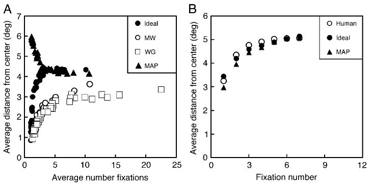
Average fixation distance from the center of the search display for human, ideal, and MAP searchers. (A) Average distance from the center of the display as a function of search task difficulty, as indexed by the average number of fixations to find the target. The data (open symbols) and ideal predictions (solid circles) are from Geisler et al. (2006). (B) Average fixation distance from the center of the display as a function of the number of saccades elapsed within the search trial in the present study (averaged across task difficulty).

We also note one other related result from the current study (Figure 6B). For human, ideal, and MAP searchers the average fixation distance from the center of the search area grows over the first few saccades within a search trial. This result is interesting because it shows another subtle aspect of rational search behavior displayed by humans. In this behavior, human searchers are more similar to the ideal than the MAP searcher (although the differences are small).

Most of the recent computational models of visual search mentioned in the introduction do not consider a foveated visual system (exceptions are Najemnik & Geisler, 2005; Peters et al., 2005). Yet, the variable spatial resolution over the visual field is the very reason why many organisms make eye movements (Carrasco, Evert, Chang, & Katz, 1995; Carrasco & Frieder, 1997; Findlay & Gilchrist, 2003; Geisler & Chou, 1995; Motter & Belky, 1998). This omission is one of the reasons we cannot simulate these computational models in our search task and obtain meaningful results to compare with ours. Another reason is that most of these models do not explicitly incorporate a source of internal variability (Eckstein, 1998), and unlike humans, they will make exactly the same eye movements when exactly the same search stimulus is presented.

Although we did not evaluate these other models by simulating their performance in our task, we tested a central underlying assumption that eye movements are directed toward locations with features similar to the target. We found that the optimal model in this family (the MAP searcher) is inadequate, at least for practiced observers in our naturalistic search task. It seems likely that our results reject other models that fixate locations based only on similarity to the target because those models will either predict performance well below human performance and/or fail to capture the qualitative properties of human fixation statistics. Instead, our results point to a more sophisticated mechanism designed to make fixations that maximize the information gained.

One class of feature-based models are those that assume fixation selection is driven from a bottom-up salience computation modulated by contextual priors or task constraints (e.g., Itti & Koch, 2000; Peters et al., 2005; Torralba et al., 2006). Although these models were primarily designed for tasks other than search for a simple known target in noise, we note that they cannot make appropriate predictions for fixation selection in our search task. In our task, the contextual priors are of minimal value because the prior probability distribution on target location is uniform. Bottom-up salience can be defined within an optimal statistical framework as a measure that is monotonic with the probability of a local image patch not belonging to the background; for example, Torralba (2003) defines salience as the reciprocal of the probability that a patch belongs to the background. A pure salience-plus-context searcher is assumed to fixate the peak of the bottom-up salience map, weighted by the context-based prior (Torralba et al., 2006). This searcher knows the statistical properties of the background, but is uncertain about specific properties of the target, and hence fixates locations having maximal probability (after weighting by the context-based prior) of not being background. Such a pure salience-plus-context searcher (or a pure salience searcher such as Itti & Koch, 2000) can be rejected as a possible model of fixation selection in our search task because the incorporation of just a small amount of uncertainty about the target shape (4 possible orthogonal target shapes, a small amount of uncertainty compared to the effective target shape uncertainty of a salience searcher) leads to the ideal searcher's performance falling well below the human performance levels (e.g., approximately 10 additional fixations in the hardest search condition and 2–3 in the easiest conditions). In order to achieve the near-optimal human performance seen in our task a salience-plus-context searcher must be upgraded to use, in the fixation–selection computation, specific knowledge of the shape of the search target. If the saliency-plus-context searcher is upgraded in this fashion it becomes essentially the MAP searcher; but, as we have seen, this searcher is rejected on other grounds.

Nonetheless, we do not wish to propose the Bayesian ideal searcher presented here as a plausible model of human visual search. For example, humans do not have perfect memory or perfect integration of information across fixations (Hayhoe, Bensinger, & Ballard, 1998; Irwin, 1991; Rensink, 2002), and it seems unlikely that the nervous system could do the calculations on the fly required for ideal fixation selection (the most complicated component of the ideal searcher). However, the fact that humans approach ideal search performance and distribute their fixations in a fashion qualitatively similar to the ideal, places very strong constraints on the possible neural mechanisms. Specifically, a plausible model for our search experiment must satisfy the following two criteria: (1) it must achieve near-optimal search performance with very little memory for visual detail, and (2) it must distribute its fixations in an approximately ideal way across the circular search area. By degrading the ideal searcher in various ways, we have begun exploring the space of possible heuristics that could satisfy these criteria.

First, in simulations we have shown that the memory capabilities of the ideal searcher (memory box in Figure 1) can be degraded substantially without significantly degrading search speed and accuracy. This is because when fixations are chosen efficiently the posterior probability rises only in the fixation or two before the target is located (Najemnik & Geisler, 2005). Thus, it is not necessary to remember or integrate the specific posterior probability values for more than a couple fixations (for evidence of integration across two fixations, see Caspi, Beutter, & Eckstein, 2004). However, the simulations also show that human performance cannot be reached without some memory for where the eyes have been (i.e., a substantial suppression of previously fixated locations). This is a much less demanding kind of memory, for which there is evidence in the literature (Aivar, Hayhoe, Chizk, & Mruczek, 2005; Klein, 1988; Rafal, Calabresi, Brennan, & Sciolto, 1989).

Second, we have derived an approximation to the procedure for ideal fixation selection that is more biologically plausible: after each saccade, the updated spatial distribution of posterior probability is convolved (filtered) with the square of the visibility map (Figure 2E) and the maximum is selected as the next fixation. For the current experiment, this procedure performs better than the MAP searcher and has fixations statistics similar to the ideal described here. The neural calculations required for this procedure are still substantial but are more plausible than those of the true ideal searcher.

Conclusions

In sum, we compared human search performance with the parameter-free predictions of a searcher that selects fixations based upon how well features detected in the periphery match the target (MAP) and with the parameter-free predictions of a searcher that selects fixations to maximize the gain of information about target location (ideal). Although the MAP searcher is representative of many current models of visual search, we find that it predicts fixation statistics that differ qualitatively from those of human searchers (Figures 3, 4, and 6). On the other hand, we find that the ideal searcher predicts fixation statistics that are qualitatively similar to those of human searchers. Our results put strong constraints on models of visual search and demonstrate that humans are sophisticated searchers who take into account how the sensitivity of their visual system varies across the retina. Search models obtained by mildly degrading the ideal searcher should provide plausible hypotheses for the underlying biological mechanisms.

References

- Aivar MP, Hayhoe MM, Chizk CL, Mruczek RE. Spatial memory and saccadic targeting in a natural task. Journal of Vision. 2005;5(3):177–193. doi: 10.1167/5.3.3. 3. http://journalofvision.org/5/3/3/ [DOI] [PubMed]
- Burgess AE, Ghandeharian H. Visual signal detection. II. Signal-location identification. Journal of the Optical Society of America A, Optics and Image Science. 1984;1:906–910. doi: 10.1364/josaa.1.000906. [DOI] [PubMed] [Google Scholar]
- Carr JC, Fright WR, Beatson RK. Surface interpolation with radial basis functions for medical imaging. IEEE Transactions on Medical Imaging. 1997;16:96–107. doi: 10.1109/42.552059. [DOI] [PubMed] [Google Scholar]
- Carrasco M, Evert DL, Chang I, Katz SM. The eccentricity effect: Target eccentricity affects performance on conjunction searches. Perception & Psychophysics. 1995;57:1241–1261. doi: 10.3758/bf03208380. [DOI] [PubMed] [Google Scholar]
- Carrasco M, Frieder KS. Cortical magnification neutralizes the eccentricity effect in visual search. Vision Research. 1997;37:63–82. doi: 10.1016/s0042-6989(96)00102-2. [DOI] [PubMed] [Google Scholar]
- Caspi A, Beutter BR, Eckstein MP. The time course of visual information accrual guiding eye movement decisions. Proceedings of the National Academy of Sciences of the United States of America. 2004;101:13086–13090. doi: 10.1073/pnas.0305329101. [DOI] [PMC free article] [PubMed] [Google Scholar]
- Curcio CA, Allen KA. Topography of ganglion cells in human retina. Journal of Comparative Neurology. 1990;300:5–25. doi: 10.1002/cne.903000103. [DOI] [PubMed] [Google Scholar]
- Curcio CA, Sloan KR, Kalina RE, Hendrickson AE. Human photoreceptor topography. Journal of Comparative Neurology. 1990;292:497–523. doi: 10.1002/cne.902920402. [DOI] [PubMed] [Google Scholar]
- Eckstein MP. The lower visual search efficiency for conjunctions is due to noise and not serial attentional processing. Psychological Science. 1998;9:111–118. [Google Scholar]
- Eckstein MP, Beutter BR, Stone LS. Quantifying the performance limits of human saccadic targeting during visual search. Perception. 2001;30:1389–1401. doi: 10.1068/p3128. [DOI] [PubMed] [Google Scholar]
- Eckstein MP, Thomas JP, Palmer J, Shimozaki SS. A signal detection model predicts the effects of set size on visual search accuracy for feature, conjunction, triple conjunction, and disjunction displays. Perception & Psychophysics. 2000;62:425–451. doi: 10.3758/bf03212096. [DOI] [PubMed] [Google Scholar]
- Findlay JM. Global processing for saccadic eye movements. Vision Research. 1982;22:1033–1045. doi: 10.1016/0042-6989(82)90040-2. [DOI] [PubMed] [Google Scholar]
- Findlay JM. Saccade target selection during visual search. Vision Research. 1997;37:617–631. doi: 10.1016/s0042-6989(96)00218-0. [DOI] [PubMed] [Google Scholar]
- Findlay JM, Gilchrist ID. Active vision. New York: Oxford University Press; 2003. [Google Scholar]
- Findlay JM, Walker RA. Model of saccade generation based on parallel processing and competitive inhibition. Behavioral and Brain Sciences. 1999;22:661–721. doi: 10.1017/s0140525x99002150. [DOI] [PubMed] [Google Scholar]
- Geisler WS, Chou Kee-Lee. Separation of low-level and high-level factors in complex task: Visual search. Psychological Review. 1995;102:356–378. doi: 10.1037/0033-295x.102.2.356. [DOI] [PubMed] [Google Scholar]
- Geisler WS, Perry JS, Najemnik J. Visual search: The role of peripheral information measured using gaze-contingent displays. Journal of Vision. 2006;6(9):858–873. doi: 10.1167/6.9.1. 1. http://journalofvision.org/6/9/1/ [DOI] [PubMed]
- Green DM, Swets JA. Signal detection theory and psychophysics. New York: Wiley; 1966. [Google Scholar]
- Hayhoe MM, Bensinger DG, Ballard DH. Task constraints in visual working memory. Vision Research. 1998;38:125–137. doi: 10.1016/s0042-6989(97)00116-8. [DOI] [PubMed] [Google Scholar]
- Honda H, Findlay JM. Saccades to targets in three-dimensional space: Dependency of saccadic latency on target location. Perception & Psychophysics. 1992;52:167–174. doi: 10.3758/bf03206770. [DOI] [PubMed] [Google Scholar]
- Irwin DE. Information integration across saccadic eye movements. Cognitive Psychology. 1991;23:420–458. doi: 10.1016/0010-0285(91)90015-g. [DOI] [PubMed] [Google Scholar]
- Itti L, Koch C. A saliency-based search mechanism for overt and covert shifts of visual attention. Vision Research. 2000;40:1489–1506. doi: 10.1016/s0042-6989(99)00163-7. [DOI] [PubMed] [Google Scholar]
- Itti L, Koch C, Niebur E. A model of saliency-based visual-attention for rapid scene analysis. IEEE Transactions on Pattern Analysis and Machine Intelligence. 1998;20:1254–1259. [Google Scholar]
- Klein R. Inhibitory tagging system facilitates visual search. Nature. 1988;334:430–431. doi: 10.1038/334430a0. [DOI] [PubMed] [Google Scholar]
- Koch C, Ullman S. Shifts in selective visual attention: Towards the underlying circuitry. Human Neurobiology. 1985;20:219–222. [PubMed] [Google Scholar]
- Lu ZL, Dosher BA. Characterizing human perceptual inefficiencies with equivalent internal noise. Journal of the Optical Society of America A, Optics, Image Science, and Vision. 1999;16:764–778. doi: 10.1364/josaa.16.000764. [DOI] [PubMed] [Google Scholar]
- Motter BC, Belky EJ. The guidance of eye movements during active visual search. Vision Research. 1998;38:1805–1815. doi: 10.1016/s0042-6989(97)00349-0. [DOI] [PubMed] [Google Scholar]
- Najemnik J, Geisler WS. Optimal eye movement strategies in visual search. Nature. 2005;434:387–391. doi: 10.1038/nature03390. [DOI] [PubMed] [Google Scholar]
- Olshausen BA, Anderson CH, Van Essen DC. A neurobiological model of visual attention and invariant pattern recognition based on dynamic routing of information. Journal of Neuroscience. 1993;13:4700–4719. doi: 10.1523/JNEUROSCI.13-11-04700.1993. [DOI] [PMC free article] [PubMed] [Google Scholar]
- Ottes FP, Van Gisbergen JA, Eggermont JJ. Latency dependence of colour-based target vs nontarget discrimination by the saccadic system. Vision Research. 1985;25:849–862. doi: 10.1016/0042-6989(85)90193-2. [DOI] [PubMed] [Google Scholar]
- Palmer J, Verghese P, Pavel M. The psychophysics of visual search. Vision Research. 2000;40:1227–1268. doi: 10.1016/s0042-6989(99)00244-8. [DOI] [PubMed] [Google Scholar]
- Pelli DG, Farell B. Why use noise? Journal of the Optical Society of America A, Optics, Image Science, and Vision. 1999;16:647–653. doi: 10.1364/josaa.16.000647. [DOI] [PubMed] [Google Scholar]
- Pelli DG, Zhang L. Accurate control of contrast on microcomputer displays? Vision Research. 1991;31:1337–1350. doi: 10.1016/0042-6989(91)90055-a. [DOI] [PubMed] [Google Scholar]
- Perry JS, Geisler WS. Gaze-contingent real-time simulation of arbitrary visual fields. In: Rogowitz B, Pappas T, editors. Human vision and electronic Imaging VII, Proceedings of SPIE. Vol. 4622 2002. [Google Scholar]
- Peters RJ, Iyer A, Itti L, Koch C. Components of bottom-up gaze allocation in natural images. Vision Research. 2005;45:2397–2416. doi: 10.1016/j.visres.2005.03.019. [DOI] [PubMed] [Google Scholar]
- Previc FH. Functional specialization in the lower and upper visual fields in humans: Its ecological origins and neurophysiological implications. Brain and Behavioral Sciences. 1990;13:519–575. [Google Scholar]
- Rafal RD, Calabresi PA, Brennan CW, Sciolto TK. Saccade preparation inhibits reorienting to recently attended locations. Journal of Experimental Psychology: Human Perception and Performance. 1989;15:673–685. doi: 10.1037//0096-1523.15.4.673. [DOI] [PubMed] [Google Scholar]
- Rajashekar U, Cormack LK, Bovik AC. In: Eye tracking research and applications. Duchowski AT, editor. New Orleans: ACM SIGGRAPH; 2002. pp. 119–123. [Google Scholar]
- Rao RP, Zelinsky GJ, Hayhoe MM, Ballard DH. Eye movements in iconic visual search. Vision Research. 2002;42:1447–1463. doi: 10.1016/s0042-6989(02)00040-8. [DOI] [PubMed] [Google Scholar]
- Rensink RA. Change detection. Annual Review of Psychology. 2002;53:245–277. doi: 10.1146/annurev.psych.53.100901.135125. [DOI] [PubMed] [Google Scholar]
- Rodieck RW. First steps in seeing. Sunderland: Sinauer; 1998. [Google Scholar]
- Rubin N, Nakayama K, Shapely R. Enhanced perception of illusory contours in the lower versus upper visual hemifields. Science. 1996;271:651–653. doi: 10.1126/science.271.5249.651. [DOI] [PubMed] [Google Scholar]
- Torralba A. Modeling global scene factors in attention. Journal of the Optical Society of America A, Optics, Image Science, and Vision. 2003;20:1407–1418. doi: 10.1364/josaa.20.001407. [DOI] [PubMed] [Google Scholar]
- Torralba A, Oliva A, Castelhano MS, Henderson JM. Contextual guidance of eye movements and attention in real-world scenes: The role of global features in object search. Psychological Review. 2006;113:766–786. doi: 10.1037/0033-295X.113.4.766. [DOI] [PubMed] [Google Scholar]
- Treisman A. Features and objects: The fourteenth Bartlett memorial lecture. Quarterly Journal of Experimental Psychology A: Human Experimental Psychology. 1988;40:201–237. doi: 10.1080/02724988843000104. [DOI] [PubMed] [Google Scholar]
- Wolfe JM. Visual search in continuous, naturalistic stimuli. Vision Research. 1994;34:1187–1195. doi: 10.1016/0042-6989(94)90300-x. [DOI] [PubMed] [Google Scholar]
- Zelinsky GJ, Rao RP, Hayhoe MM, Ballard DH. Eye movements reveal the spatiotemporal dynamics of visual search. Psychological Science. 1997;8:448–453. [Google Scholar]
Associated Data
This section collects any data citations, data availability statements, or supplementary materials included in this article.