

Abstract
We use the temporal asymmetry of the cross-correlation function to determine the temporal ordering of spatially localized cellular events in live-cell multichannel fluorescence imaging. The analysis is well suited to noisy, stochastic systems where the temporal order may not be apparent in the raw data. The approach is applicable to any biochemical reaction not in chemical equilibrium, including protein complex assembly, sequential enzymatic processes, gene regulation, and other cellular signaling events. As an automated quantitative measure, this approach allows the data to be readily interpreted statistically with minimal subjective biases. We first test the technique using simulations of simple biophysical models with a definite temporal ordering. We then demonstrate the approach by extracting the temporal ordering of three proteins—actin, sorting nexin 9, and clathrin—in the endocytic pathway.
Introduction
Cell behaviors generally are triggered by specific combinations and temporal sequences of molecular signaling events. For instance, molecules can behave as switches: the association of an upstream protein to a receptor or signaling complex in turn can trigger downstream proteins to associate (e.g., by posttranslational modifications like phosphorylation or ubiquitylation, or by protein conformation changes). These pathways are typically complex, often with only weak and transient interactions between the components, and they occur in an intrinsically noisy biochemical environment. Sorting out and understanding cellular pathways is one of the grand challenges of biology (1–3).
Recent advances in live-cell multichannel fluorescence imaging have made possible the direct observation of spatial and temporal dynamics of cellular events (4). In practice, these observations are typically made by visual inspection, a process made problematic by subjective errors and biases, noise from the camera and background fluorescence, difficulty in obtaining quantitative information, and limitations to the amount of data that can be processed in this manner.
Algorithmic approaches have the potential to overcome these limitations. One recent advance has been to apply machine-learning Bayesian inference to high-throughput multichannel flow cytometry experiments (5), in which information about cellular pathways can be obtained automatically and aggregated from static snapshots of a large statistical sample of cells. Older algorithmic approaches include correlation spectroscopies, such as fluorescence correlation spectroscopy (FCS), which use the correlation function to measure dynamics and interactions reflected in microscopic measurements of fluorescence intensity. Correlation functions are a way to quantitatively aggregate information from noisy, stochastic time series; when applied to fluorescent movies, they operate directly on intensity values and do not require individual molecules or particles (e.g., speckles) to be resolved.
Here, we apply a fluorescence correlation approach that uses asymmetries in the temporal cross-correlation function to gain information about the temporal ordering in cellular reaction networks, similar to the approach proposed by Qian and Elson (6), which built on the observation that temporal asymmetries in correlation functions signify nonequilibrium processes (7). Our approach operates on the more experimentally accessible protein species, however, rather than the biochemical state. Qian and Elson (6) show that the shape and asymmetry of the cross-correlation function can measure the biochemical flux, which quantifies the degree to which a reaction network is out of equilibrium. Nearly all reaction network subsystems in living cells operate out of equilibrium, and nonequilibrium fluxes are required for temporal ordering. Protein recruitment, sequential enzyme reactions, gene regulation, protein complex assembly, and most cellular signaling events are examples of nonequilibrium reactions.
Two analysis techniques closely related to the approach described here are image cross-correlation spectroscopy (ICCS) and fluorescence cross-correlation spectroscopy (FCCS). Both of these techniques fall into the larger category of fluctuation correlation analyses, and are two-channel (cross-correlation) versions of more common single-channel (autocorrelation) techniques. FCCS, first performed by Schwille (8), uses temporal cross-correlation and extends FCS (9), whereas ICCS uses spatial cross-correlation and extends image correlation spectroscopy (ICS) (10). FCCS has been used to determine enzyme kinetics and activities (11) and to study protein-protein interactions (12) and endocytosis (13). It obtains mobility information in addition to degree of colocalization (14). The approach presented here differs from ICCS, FCCS, and other fluctuation analyses in that its focus is determining the temporal ordering rather than mobility or simple colocalization.
We first illustrate the technique using a simple Monte Carlo simulation of two types of proteins interacting at stationary states, producing a colocalization with a definite temporal ordering (see Materials and Methods). Using the simulation, we illustrate and quantify the sensitivity of the technique. We then demonstrate the efficacy of the analysis for multichannel fluorescence live-cell imaging of proteins in the endocytic pathway, reproducing the reported temporal ordering from the literature.
Theory
Correlation function
The temporal cross-correlation function (hereafter, simply the correlation function) is defined as
| (1) |
where the angled brackets indicate an average over time t, (similar for ), τ is the time shift, and A is a normalization constant, chosen to be the inverse geometric mean of the variances divided by the means . In the situation considered below, X(t) and Y(t) are fluorescence intensity time series of two color channels in a single spatial region.
The correlation can also be expressed in terms of probabilities (15):
| (2) |
where the sums are over discrete bins of intensity X = {x1, x2,…, xN} (similarly for Y). is the conditional probability of Y(τ) given X(0), and pX and pY are the probability distribution functions of X(t) and Y(t). The probabilities are obtained from the fraction of time points in the appropriate bin.
The interpretation of the correlation is simplest when there is only one of each particle type and when the intensity time series is binary, so that 0 or 1 indicates whether a particle is absent or present, respectively, in the region of interest. The correlation then simplifies to
| (3) |
When , the X and Y channels are statistically independent, implying that the labeled molecules do not interact. Thus, the sign of CC(τ) gives the degree of colocalization relative to statistical independence.
With more particles (requiring more than two intensity bins), the τ-dependent conditional probabilities are weighted by the intensity value of each bin, so that the correlation measures the linear dependence between X and Y. In practice, the correlation is computed using the fast Fourier transform, and the bins are effectively continuous.
The statistical interpretation of the correlation function (Eqs. 2 and 3) generalizes the concept of colocalization. Colocalization typically refers to the degree to which two proteins appear at the same location at the same time. Here, colocalization is expanded to be a function of time lag: given a particle of type A at time t = 0 at a particular stationary spatial location, how likely are particles of type B to be at that same location at ?
Correlation function characterizes colocalization and temporal ordering
The correlation is also usefully interpreted graphically. Consider a simplified schematic for the fluorescence intensity signal from a single cellular binding event pair (Fig. 1 a). In general, a signal will be the addition of many such events, occurring stochastically. In the single event, suppose an upstream protein binds and produces a fluorescent pulse signal in the X channel of intensity h1. (The signal is assumed to be sensitive only to the presence of a bound protein and is determined by details of the system, like laser intensity, camera sensitivity, etc.). After a time, tlag, the signal is followed by a pulse in the Y channel from a downstream protein binding and colocalizing; the protein complex then unbinds and the two signals decay together.
Figure 1.
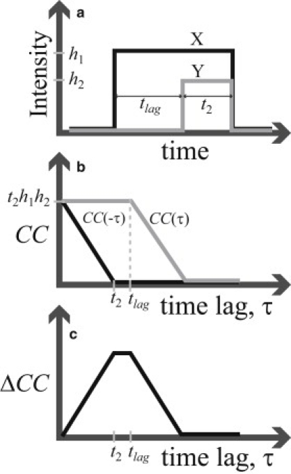
Idealized signaling event illustrating how relevant features appear in the correlation function. Each molecule in the X (Y) channel produces intensity h1 (h2) when bound, and zero intensity otherwise. (a) A binding event occurs in the X channel (black) first, followed by an event in the Y channel (gray) at a time tlag later; the two events then unbind simultaneously. (b) The cross-correlation for positive (gray) and negative (black) time lag, which is not symmetric in time. (c) The cross-correlation difference, ΔCC, characterizing the temporal asymmetry.
The correlation is easily calculated using Eq. 1 and is shown in Fig. 1 b as a function of time lag. The time lag, τ, is a shift in time of one channel relative to the other, and is independent of when the event pair occurs in time (the temporal distance from the origin in Fig. 1 a). This feature allows the conditional statistical interpretation above: given a signal in one channel, what is the probability of a signal in the other channel occurring at some time τ earlier or later? The sign of the correlation gives the type of colocalization compared to statistical independence: positive, negative, or independent.
To have a consistent temporal ordering, there has to be a temporal asymmetry in the correlation, which is quantified by the correlation difference: (Fig. 1 c), where τ is restricted to positive values, so that represents the colocalization at time τ earlier. Note that is equivalent to the positive time lag correlation with the channels switched; i.e., . ΔCC thus characterizes the temporal asymmetry of the correlation function. It is significant that a nonzero ΔCC implies a colocalization probability current. This notion of current is already reflected in the standard biological use of the terms upstream and downstream.
We can also see that the relevant timescales, tlag and t2, appear as corners (time points with discontinuity in slope) in CC(τ) and ΔCC. However, since tlag and t2 will typically be random variables described by probability distributions, the relevant corners will be smoothed into a continuous curve in a generally complicated way, potentially depending on the dynamics of the whole network. Thus, the relative timing may be difficult to clearly resolve. One source of this difficulty is that the relative timing is naturally defined by transitions, whereas the fluorescence intensities inherently reflect colocalization states. The transitions could in principle be found by taking the derivatives of the intensity time series, but imaging noise makes this impractical. In conclusion, peaks in ΔCC (e.g., those in Fig. 2, b and d; see also Fig. 4 h), though intuitively suggestive, should not be interpreted as simply characterizing the relative timing.
Figure 2.
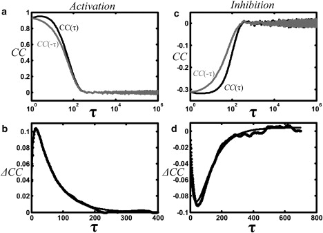
Cross-correlation analysis of simulations. (a) For activation, the cross-correlation, CC(τ), for positive τ (black) and negative τ (gray) are both positive, indicating positive colocalization for all τ. (b) (corresponding to the difference between the curves in a) is also positive for all τ, correctly identifying the X channel as upstream. The simulation parameters were T = 2 × 10⁶ time points, L =127, Lsite = 1, D = 25, N = 100 particles, and there was one binding site. The rate constants are defined as in Eq. 6, with = .015, =.0001. (c and d) Same as a and b, but for inhibition, where . CC(τ) is negative for all τ, indicating negative colocalization. ΔCC(τ) is negative, correctly indicating that X is upstream. The smooth curves in b and d are fits to the functional form for ΔCC(τ) derived in the Appendix: , where A,, and are fitting parameters.
Figure 4.
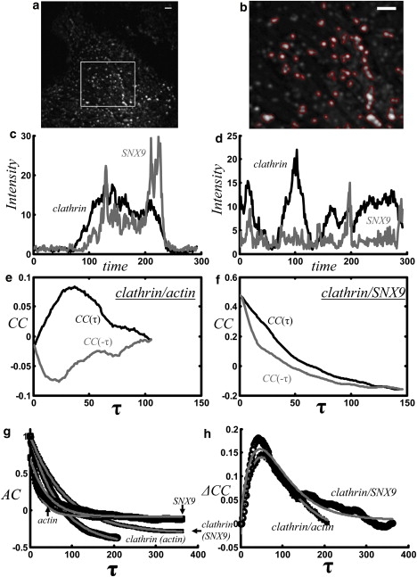
Correlation analysis of clathrin, SNX9, and actin in the endocytic pathway. (a) Temporal average of the clathrin channel after application of a rolling ball filter (radius = 9 pixels), showing one cell. (b) An arbitrary subregion in a is shown overlaid with the outline of the cluster mask. There are 155 clusters identified in the whole image. Pixels within each cluster are summed for each time point, producing a separate intensity time series for each cluster. Scale bar (a and b), 2 μm. (c) Fluorescence-intensity time series from a pixel cluster for clathrin (black) and SNX9 (gray), where the expected relationship is evident in the time series. (d) Same as c, except for a pixel cluster with no apparent temporal relationship between clathrin and SNX9. The time series are divided by the spatial mean of the whole image at each time point to compensate for photobleaching. (e) Average correlation for positive (black) and negative (gray) time lag between clathrin and actin is 1), approximately zero for zero time lag; 2), positive when the clathrin channel is shifted forward in time; and 3), negative when the clathrin channel is shifted backward in time. (f) The average correlation between clathrin and SNX9 averaged over clusters is positive, indicating positive colocalization at all times. (g) All four autocorrelations decay approximately exponentially with decay constants: τ = 71 s, clathrin (actin experiment); τ = 25 s, actin; τ = 88 s, clathrin (SNX9 experiment); and τ =42 s, SNX9. Because the experiment times are comparable to the correlation times, the correlations in e and f are negative for later time shifts. This is because a zero-mean time series will have a zero-mean autocorrelation, and thus, positive correlations at early time lags will be offset by negative correlations at larger time lags. (h) ΔCC is positive for both experiments, suggesting that clathrin is upstream of both actin and SNX9. Fits to the functional form of the model in the Appendix show remarkable agreement with the data, considering the simplicity of the model.
Simple models for temporal ordering of colocalization
We consider two types of generalized colocalization relevant for multispecies cellular processes: activation and inhibition. In activation, an upstream molecule binds and causes downstream molecules to positively colocalize. Examples of activation include recruitment and protein complex assembly. In inhibition, the upstream molecule causes downstream molecules to be negatively colocalized, as in competitive binding events. The terms cause and upstream/downstream in this context imply a nonequilibrium process and the dissipation of energy, which are required for temporal ordering.
The ordering is obtained from the sign of ΔCC and the type of colocalization. For activation, the term —and, thus, ΔCC—is positive when X is upstream and Y is downstream, because a bound upstream particle increases the probability for future binding compared to past binding of the downstream particle, but not vice versa. For inhibition, the same reasoning makes the same ordering correspond to negative ΔCC. If the colocalization is independent, there is no ordering and ΔCC is zero.
Integrated cross-correlation
The correlation typically varies with time lag and for some ranges fluctuates around zero, potentially making the sign determination difficult with limited statistics or noisy data (e.g., see Fig. 2, c and d). However, the sign determination can be made quantitative and more sensitive if the correlation and correlation difference are first summed over a range of τ:
| (4) |
| (5) |
where choosing τmax to be near the correlation time maximizes the signal/noise ratio (see Fig. 3 c), but all available lag times may be used.
Figure 3.
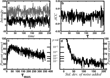
Summing correlation difference increases the robustness of temporal order determination. Gaussian noise with standard deviation σ is added to simulated intensity time series pairs (underlying time series has a standard deviation of 5 intensity units). The parameters are the same as in Fig. 2a, except there are N = 100 sites and T = 8192. For σ = 25, temporal ordering is not evident visually in either the time series (a) (one channel offset for clarity) or the correlation difference, ΔCC(τ) (b). Nonetheless, summing the correlation difference from τ = 0 to τ = τmax and taking the sign (see Methods) reliably indicates the temporal ordering. The fraction of sites with the correct sign is determined, and the probability of obtaining that fraction from random signals gives the p-value for (c) variable τmax (with σ = 25) and (d) variable noise level (with τmax = 50).
Materials and Methods
Cell culturing and transfection
BSC1 stably expressing clathrin light-chain green fluorescent protein (GFP-clathrin) cells (1 × 10⁵) (a gift from T. Kirchausen, Harvard Medical School, Cambridge, Massachusetts) were plated onto 22 × 22-mm glass coverslips (Corning, Corning, NY). The next day, cells were microinjected with X-rhodamine-labeled G-actin (∼1 mg/ml) and imaged 2–4 h postinjection using total internal reflection fluorescence microscopy (TIR-FM). For imaging mCherry-sorting nexin 9 (mCherry-SNX9), 8 × 10⁴ BSC1 GFP-clathrin cells were plated onto coverslips, allowed to attach overnight, and transfected with mCherry-SNX9 DNA using Lipofectamine 2000 (Invitrogen, Carlsbad, CA) according to the manufacturer's instructions. Cells were imaged 16–20 h posttransfection. Cells were viewed with an inverted microscope (TE2000U, Nikon, Tokyo, Japan) custom modified to allow for through-the-objective TIR-FM using a 100×, 1.45 NA objective (Nikon) (system previously described in Yarar et al. (16).). An evanescent field depth of ∼200 nm (calculated from the angle of the light) was used for the experiments. Images were collected using an Orca II-ERG camera (Hamamatsu, Shimokanzo, Japan) operated in 14-bit mode. Stage temperature was maintained at 35°C with a custom-modified stage incubator. Cells were imaged in DMEM (no phenol red), 10 mM HEPES, pH 7.5, 10% fetal bovine serum, and 1.0 U/ml oxyrase. Consecutive red and green TIR-FM (150- to 500-ms exposure) images were taken for 10 min for either GFP-Clathrin and X-rhodamine-actin (2-s intervals) or GFP-Clathrin and mCherry-SNX9 experiments (2.5-s intervals).
Isolating sites where proteins of interest collect
The analysis assumes that the structures are spatially localized. If these structures move, the correlation will also contain information about the mobility of the structures, complicating the analysis. Although this mobility information is often important, it can be determined separately using established techniques, such as FCS or particle tracking.
To eliminate the effect of structure motion, pixels are summed in clusters that confine structures (see Fig. 4 a). These pixel clusters can be found using one of the many methods of image segmentation (17). The segmentation used here began with a temporal average of the movie in which the background was removed using a rolling-ball filter (17) in ImageJ. The H-maxima transform (imhmax in MATLAB's Image Processing Toolbox, The MathWorks, Natick, MA) was applied to suppress maxima with intensity peaks less than a parameter h. We chose h to be 2.5 times the standard deviation of the average image. The transformed image was then thresholded using the same intensity value h. Using the built-in MATLAB function bwlabel, connected regions in the binary image were labeled, defining the clusters. The correlations for each pixel cluster were then averaged together to improve statistics.
Computer simulations
Simple two-channel Monte Carlo simulations of 1D diffusion with binding at discrete sites were custom-written in MATLAB. In all simulations, two types of particles, A and B, represented upstream and downstream proteins. For each time step, the position of unbound particles was advanced by adding a random floating point number picked from a zero mean Gaussian distribution with standard deviation, where is the time step and D is the diffusion coefficient (in units of ΔL2 /Δt, where ΔL is a length unit). Each particle had the same diffusion coefficient D.
In each time step, particles became bound when their positions overlapped with a binding site (i.e., the on-rate, , was diffusion-limited). Bound particles escaped with a probability/time step that depended on the particle type and, for downstream particles, the presence or absence of the upstream species:
| (6) |
Particles that escaped the energy barrier then diffused in the same time step.
Time series of model fluorescent signals were generated by summing the number of particles at each binding site. To test the noise sensitivity, possible sources of noise (read noise, background fluorescence, etc.) were simulated by adding Gaussian white noise to each time series.
The binding sites were of width Lsite = 1 and were placed evenly along the system length L. Simulations illustrating the shape of ΔCC (see Fig. 2) used only one binding site, whereas those testing the noise sensitivity (see Fig. 3) used N = 100. The particles were initially randomly placed with uniform probability and then allowed to relax to the steady-state particle distribution for 5000 time steps before starting the simulation.
In the simulation, the total number of particles was fixed; however, the system is implicitly out of thermodynamic equilibrium, as reflected in the values of the on-rates and off-rates, and , which in turn reflect differences in free energy, , where R is the gas constant. For an isolated system consisting only of sites and A and B particles, the free-energy difference between the state with neither A nor B bound and the state with both A and B bound must be independent of whether the upstream or downstream molecule binds first, but in Eq. 6, this is not so. Thus, consistency with thermodynamics requires an implicit inclusion of other particle species to account for the changes in probabilities that reflect the activation or inhibition. Furthermore, to have a well-defined temporal ordering, the concentrations of these other particles must be out of equilibrium (e.g., physiological levels of ATP).
Results
Simulation results
Correlations from the binding model simulations are shown in Fig. 2 and are described by the expression derived in the Appendix. For the activation simulation (see Methods), the sign of is positive, reflecting the expected positive colocalization (Fig. 2 a). The sign of is also positive (Fig. 2 b), reflecting the temporal ordering: X upstream and Y downstream. For the inhibition simulation, the sign of is negative, reflecting the expected negative colocalization (Fig. 2 c), and the sign of is negative (Fig. 2 d), reflecting the temporal ordering: X upstream and Y downstream.
Fig. 2, b and c, also shows the fit to Eq. 12 (see Appendix): , where CC(0), τ0, and τ1 are fitting parameters. The best-fit values for the two timescales are τ0 = 62.6 and τ1 = 11. These values are consistent with τ0 = = 66.7, the mean binding time of the upstream particle, and , the mean time for the downstream particle to bind after the upstream particle binds (see Appendix). Though similar in this example, the relative timing is not simply the peak of ΔCC, which occurs at = 20.
Ordering and interaction mechanism determinations are robust to noise
To determine the sensitivity of the technique to noise, a binding simulation (activation) was performed as above, but with 100 independent binding sites. The temporal ordering at each site was determined in the presence of noise from the sign of calculated from the time series at that site (Fig. 3). White Gaussian noise with standard deviation σ = 25 is added to the intensity time series for each channel of a cluster (Fig. 3 a) and ΔCC(τ) is calculated (Fig. 3 b); for this value of σ, the noise completely obscures the dynamics, including any apparent temporal ordering. The fraction of sites that produced the correct ordering was measured from the sign of , as a function of the maximum time lag, , over which ΔCC(τ) is summed (Fig. 3 c). The fraction correct reaches a maximum soon after the peak in ΔCC(τ), which occurs at = 20 (see Fig. 2 b). Fig. 3 d shows the fraction of correct sites as a function of added noise strength, with . The determination of the mechanism (activation versus inhibition) shows similar noise sensitivity.
As shown in Fig. 3, c and d, the fraction of sites with correctly identified temporal ordering was converted to a p-value to quantify its statistical significance. The p-value gives the probability of obtaining at least as many correct order determinations as observed, assuming the null hypothesis that there was no ordering. Without ordering, would have positive or negative sign with equal probability, and the number of trials with either outcome would be a binomial random variate with probability 1/2.
It is significant that the determination can be made confidently (low p-value) even when no relation is apparent in the time series (Fig. 3 a) or correlation (Fig. 3 b). Note that the p-values even for these noisy data are orders of magnitude lower (better) than the conventional threshold for statistical significance, p < 0.05. Nonetheless, such noisy data, producing a cross-correlation function with no apparent shape, should be interpreted with caution.
Analysis of endocytic pathway live-cell imaging reproduces known temporal relationships
Fig. 4 shows the results of the cross-correlation analysis for two different two-channel live-cell fluorescent movies of the endocytic pathway: GFP-Clathrin (clathrin)/mCherry-SNX9, and GFP-Clathrin/X-rhodamine-actin. For the experiment in which GFP-Clathrin and X-rhodamine-actin were imaged simultaneously in an individual cell, Fig. 4 a shows the temporal average of the time-lapse GFP-Clathrin movie used to generate the corresponding cluster mask (Fig. 4 b, outlined clusters). There were 155 distinct clusters. For the experiment in which GFP-Clathrin and mCherry-SNX9 were imaged simultaneously in an individual cell, there were 182 clusters. The value of the thresholds changed the number of clusters but did not qualitatively change the results.
Fig. 4, c and d, shows two examples of the fluorescence-intensity time series of GFP-Clathrin and mCherry-SNX9 at single endocytic events; timing relationships from the raw movies and the intensity time series of the clusters can sometimes be determined by eye (e.g., Fig. 4 c, in which SNX9 appears to accumulate after clathrin) but often not (e.g., Fig. 4 d, in which the two time series appear unrelated). Correlation techniques, however, can aggregate the data in a reproducible, systematic way without subjective bias.
Here, the correlation is computed for each cluster and then averaged over clusters. As seen in Fig. 4 e, the average correlation between clathrin and actin is 1), approximately zero for zero time lag, 2), positive when the clathrin channel is shifted forward in time, and 3), negative when the clathrin channel is shifted backward in time. These three features imply that 1), at any given time, actin and clathrin colocalize approximately randomly, 2), the presence of clathrin predicts positive colocalization of actin in the future, and 3), the presence of clathrin predicts negative colocalization of actin in the past. In an equivalent manner, implications 2 and 3 could be described in reference to the presence of actin, which would predict positive colocalization with clathrin in the past and negative colocalization with clathrin in the future. As seen in Fig. 4 f, the correlation between clathrin and SNX9 averaged over clusters is positive, indicating that clathrin accumulates on the plasma membrane with SNX9 (i.e., positive colocalization) at all times. The asymmetry in the correlation indicates that on average, clathrin appears before SNX9. The lack of a negative correlation suggests that clathrin and SNX9 dissociate from the plasma membrane simultaneously.
The average autocorrelations of all four signals are approximately exponential decays (Fig. 4 g), suggesting that the probability of clathrin-coated pit appearance and disappearance is roughly independent of time. Since the diffusive motion of the clathrin-coated pits (D ∼ 10−4 μm2/s, determined by particle tracking; data not shown) has been eliminated, the correlations reflect the dynamics of accumulation and internalization, not motion.
Discussion
Clathrin-mediated endocytosis is a multistep process in which proteins, including clathrin, assemble onto the cell membrane to form clathrin-coated pits. Coated pits subsequently mature, invaginate, and pinch off from the plasma membrane to form clathrin-coated vesicles that move into the cell. Endocytosis is highly regulated and involves the coordinated functions and recruitment of >30 accessory proteins. However, the assembly hierarchy of many of these factors has not been quantitatively analyzed.
In previously published works, the temporal order of accumulation at sites of endocytosis at the plasma membrane of three proteins—clathrin, actin, and SNX9—was determined subjectively by hand analysis of two-color time-lapse image series (16,18). Using the same data, by systematically including all data in an algorithmic way, we reproduced the finding that clathrin accumulation precedes both actin and SNX9 accumulation at endocytic vesicles. The masked clusters, defined using the clathrin channel, corresponded to the accumulation of fluorescent actin and SNX9, as evidenced by the significant correlations in Fig. 4. Presumably, each cluster contains one or (in some cases) several sites on the plasma membrane where a clathrin-coated pit forms and then pinches off to form a vesicle.
The automated segmentation procedure allowed a more comprehensive description of the colocalization in terms of the correlation (Fig. 4, e and f). The generalized colocalization (which implicitly includes the temporal ordering) could be equivalently described by the nonequilibrium biochemical flux between appropriately defined biochemical states (6,19,20).
The correlation for clathrin/SNX9 (Fig. 4 f), which is largely positive, is consistent with our simple activation binding model. The correlation for clathrin/actin (Fig. 4 e), which is both positive and negative, is more complicated. The correlation implies both that clathrin activates actin, and that actin inhibits clathrin. Both descriptions are consistent with a model in which clathrin-coated pits recruit actin, which then induces internalization.
The terms activation and inhibition, which described the simple models used in the computer simulations (see Methods), can refer to a broader class of interactions than those considered here. For instance, the inhibiting molecule (the upstream molecule in the inhibition simulation) could trigger a cascade of events that inhibit the downstream molecule after the upstream particle has left the site. In this case, the colocalization could be positive for some time lags, unlike the inhibition model considered here, which is always negatively colocalized. Furthermore, the temporal ordering would depend on the details of how the system was maintained out of equilibrium.
The possibility of cyclic processes introduces additional complications and potentially makes the temporal ordering ambiguous: two proteins could mutually activate or inhibit each other, possibly with one or more intervening interactions. This ambiguity disappears, however, if the cycle time is much longer than either the observation time or the longest autocorrelation timescale. In both the clathrin/actin and clathrin/SNX9 experiments, the autocorrelations were all monotonically decaying functions, indicating no significant cyclic processes occurring at the timescale of the experiments.
The average correlation difference, ΔCC, for both experiments has been fit to the functional form of the model derived in the Appendix (see Fig. 4 h). Although the fit correspondence suggests that the simple model is relevant to our biological system, we leave a more careful analysis for future work, which would likely require more realistic modeling. Because of the large space of possibilities, these models would be inspired by specific biological hypotheses. We also note that our model does not adequately describe most correlation curves from individual clusters (data not shown). Indeed, about a quarter of the individual cluster curves have an apparent temporal ordering opposite that shown by the average correlation (see Table 1). This discrepancy is likely due to low-frequency noise caused by poor statistics at the individual cluster level, as the experiment times are comparable to the mean lifetime of a clathrin-coated pit (see Fig. 4 h) and each cluster contains, at most, several pits. A reliable correlation would only be expected with a large number of events, which for the data in this study occurs only when the correlation curves from many clusters are averaged together.
Table 1.
Results for endocytic pathway temporal order determination
| Normal pairing |
Randomized pairing |
||||
|---|---|---|---|---|---|
| Same/opposite | p-value | Same/opposite | p-value | ||
| Actin/clathrin | 56 s | 105/48 | 10−6 | 69/84 | 0.9 |
| SNX9/clathrin | 70 s | 148/32 | <10−13 | 92/88 | 0.6 |
The biological significance of these findings is that they imply that clathrin accumulation causally activates the subsequent accumulation of actin and SNX9, leading to the internalization of an endocytic vesicle. Since it is known that SNX9 is involved in activating the polymerization of actin filaments, it would be interesting to know the temporal relationship describing the accumulation of these proteins as analyzed by this new method.
Guidelines for future applications
There are several ways in which useful future applications of the approach might differ from this study. First, the images analyzed could be acquired using another imaging modality (e.g., confocal, widefield fluorescence), not just TIR-FM; and the images could be acquired at any available frame rate. The technique aggregates correlated events occurring within the temporal resolution of the time-lapse images. In practice, this resolution is limited at short timescales by the maximum available frame rate of the camera, adequate photon statistics, and other relevant parameters of high-speed microscopy, and at long timescales largely by cellular behavior, such as movement of cells outside the field of view, or dividing of cells.
Second, the regions of interest (ROIs) (the clusters in our study) could be determined using other segmentation strategies, based, for example, on visible cellular structures (21), which could be in highly processed images (e.g., maps of temporal variance), not just the original-intensity images. ROIs could be identified by hand, or using a third imaging channel (e.g., a stain to identify the nucleus), or could even be an entire cell, in which case colocalization would represent global changes in protein synthesis or degradation. Finally, related cross-correlation methods (22) could also be used to identify regions of interest.
ROIs could be tracked to allow them to move relative to the sample frame. In our study, we tracked the clusters using techniques from multiple particle tracking (data not shown), but the small displacements of the clusters allowed this step to be removed for simplicity, without noticeable effect on the analysis results.
The segmentation step might be eliminated entirely, particularly if the sites of event activity are not optically resolvable. ROIs could be simply each pixel (or binned pixels), or a single diffraction-limited spot, as in standard FCS. If the biochemical reactions occurred on objects that diffused, temporal asymmetry could be observed if the time for the objects to move through a region was slow compared to the characteristic time of the reaction. Without visible structures, control measures to rule out spurious sources of correlation, such as photobleaching or cross talk between fluorescent channels, become especially prudent.
As a final note, the control procedure used to assess the significance of temporal asymmetry should readily transfer to other applications. In particular, pairing an ROI from one channel with a random region in the other channel (see Results) is a quick way to determine the significance of global intensity variations, such as different photobleaching rates or fluctuating illumination sources, which can produce confounding temporal asymmetry. The expected statistical significance could be determined from a comprehensive consideration of event and photon statistics, and other sources of noise, which are similar to those for other correlation techniques (23).
Conclusions
We have applied a new approach to determine the temporal ordering of spatially localized events from noisy live-cell multichannel fluorescence movies. The sign of the correlation function describes a generalized colocalization, and the sign of the temporal asymmetry describes the direction of nonequilibrium biochemical flux, i.e., identifies upstream and downstream channels. The temporal ordering determination was robust to noise, and possible when no apparent relationship was apparent in the time series or correlations. The approach was then applied to a biological system for the first time using two-channel live-cell movies of fluorescently labeled proteins in the endocytic pathway.
In this system, the sites of protein accumulation were not stationary due to the diffusion-like motion of the clathrin-coated pits. To isolate the binding dynamics in the time series, localized pixel clusters were identified using a type of image segmentation applied to the temporal average of movies; the intensities of the pixels in the cluster sites were then summed together.
We believe that this approach can be usefully developed further and applied to a wider range of biological systems, and that it fills a niche between the approaches of molecular biology and systems biology.
Appendix: correlation for simple 1D activation cell-signaling model
In this section, we find an analytical solution for the correlation for a simple activation-like model. We further show that there are two timescales in the problem and find explicit expressions for them. The solution provides a means for rigorous interpretation of the cross-correlation results from the simulation and should guide similar analyses of more realistic models.
Consider a single binding site and two particles of different type: one upstream (X channel), and one downstream (Y channel). The model system is 1D, has a total length L, and has periodic boundary conditions. The binding site has length Lsite. Upstream particles bind weakly when they land in the site, and they unbind with a fixed probability, , for each time step, giving the wait-time distribution for unbinding: , where the time is the inverse of the rate constant . The downstream particle freely diffuses through the binding site when no upstream particle is present, but otherwise binds strongly, so that the downstream particle unbinds only when the upstream particle unbinds. (Note that the binding and unbinding probabilities depend on the free-energy difference between the states (A, B, AB) and that the free-energy difference from an unbound site to AB must be independent of path—i.e., whether A or B binds first. Thus, the probabilities above imply the presence of other particles for the model to be thermodynamically consistent.)
When an X particle is bound at t = 0, the probability of it being bound at time τ decays symmetrically for positive and negative τ. The key asymmetry in the problem is with respect to the time t = 0 when an X particle is bound and concerns Y particles unbound at t = 0. In particular, for positive τ, the probability that the unbound Y particle is bound increases, whereas for negative τ, the probability remains constant at the simultaneous joint probability pY(0)|X(0).
Although the X particle is bound, the binding of the Y particle unbound at t = 0 to bind at time τ is a first-passage problem. The binding probability (normalized rate of binding) is given by Redner (24):
| (7) |
where s is the Laplace frequency, L is the system size minus the binding site length, D is the diffusion coefficient, and x0 is the position of the Y particle at t = 0. Since unbound particles are equally likely to be anywhere on the interval, the average binding probability is
| (8) |
The inverse Laplace transform of Eq. 8 then gives the time-dependent binding rate. The appropriate probability for the correlation is not the binding rate, however, but the probability of being bound at τ, so should be integrated from 0 to τ.
We can now write expressions for the conditional probability for the two time directions:
| (9) |
The terms in the square brackets give the increase in probability for a Y particle to be present at t = τ given an X particle at t = 0; its contribution to the conditional probability for both directions of τ is multiplied by the exponentially decaying probability for the X particle to be bound. The simultaneous joint probability, pY(0)|X(0), depends on the ratio of the site length to the total length, and the binding strength of the X particle.
The third term in the square brackets, present only for positive τ, is the asymmetric piece. The inverse transform can be approximated by first approximating Eq. 8 as
| (10) |
which has a known closed-form inverse transform
| (11) |
where τ1 and a are positive constants that can be determined by expanding both and in s and equating pairs of terms, giving and (the prefactors depend weakly on which terms in the expansion are used but are of order 1). Integrating Eq. 11 from zero to time lag τ is then
where Erf[] is the error function.
We can now compute the correlation difference by substituting the above integral for the approximate inverse Laplace transform into Eq. 9:
| (12) |
This expression is composed of two separable time-dependent contributions: the error function piece, resulting from the binding of the Y particle after activation by the X particle, and the exponentially decaying piece, resulting from the unbinding of the X particle. The binding after activation is described by the timescale τ1 (the time for the error function to saturate), which depends on the diffusion coefficient, the system size, and the mean number of unbound downstream particles: . (If τ1 is comparable to or larger than τ0 or the experiment time, then , and τ1 is no longer relevant to the shape of the correlation.)
The timescale τ0 depends on the binding strength of the X particle. Since the X channel is independent of the Y channel, the exponentially decaying piece can be obtained from the autocorrelation of the upstream channel:
So both relevant timescales can in principle be obtained from the correlations.
Acknowledgments
We acknowledge helpful conversations with Jim McNally, Alexander Lobkovsky, Susette Mueller, Erin Rericha, Paul Roepe, and Tim Stasevich.
This project was supported by National Science Foundation grant DBI-0353030 and Air Force Office of Scientific Research grant FA9550-07-1-0130.
Footnotes
Danial R. Sisan's present address is Biochemical Science Division, National Institute of Standards and Technology, Gaithersburg, MD 20899.
References
- 1.Hensley K., Robinson K.A., Floyd R.A. Reactive oxygen species, cell signaling, and cell injury. Free Radic. Biol. Med. 2000;28:1456–1462. doi: 10.1016/s0891-5849(00)00252-5. [DOI] [PubMed] [Google Scholar]
- 2.Irish J.M., Kotecha N., Nolan G.P. Mapping normal and cancer cell signalling networks: towards single-cell proteomics. Nat. Rev. Cancer. 2006;6:146–155. doi: 10.1038/nrc1804. [DOI] [PubMed] [Google Scholar]
- 3.Laufs U., Liao J.K. Targeting Rho in cardiovascular disease. Circ. Res. 2000;87:526–528. doi: 10.1161/01.res.87.7.526. [DOI] [PubMed] [Google Scholar]
- 4.Giepmans B.N.G., Adams S.R., Tsien R.Y. The fluorescent toolbox for assessing protein location and function. Science. 2006;312:217–224. doi: 10.1126/science.1124618. [DOI] [PubMed] [Google Scholar]
- 5.Sachs K., Perez O., Nolan G.P. Causal protein-signaling networks derived from multiparameter single-cell data. Science. 2005;308:523–529. doi: 10.1126/science.1105809. [DOI] [PubMed] [Google Scholar]
- 6.Qian H., Elson E.L. Fluorescence correlation spectroscopy with high-order and dual-color correlation to probe nonequilibrium steady states. Proc. Natl. Acad. Sci. USA. 2004;101:2828–2833. doi: 10.1073/pnas.0305962101. [DOI] [PMC free article] [PubMed] [Google Scholar]
- 7.Steinberg I.Z. On the time reversal of noise signals. Biophys. J. 1986;50:171–179. doi: 10.1016/S0006-3495(86)83449-X. [DOI] [PMC free article] [PubMed] [Google Scholar]
- 8.Schwille P., Meyer-Almes F.J., Rigler R. Dual-color fluorescence cross-correlation spectroscopy for multicomponent diffusional analysis in solution. Biophys. J. 1997;72:1878–1886. doi: 10.1016/S0006-3495(97)78833-7. [DOI] [PMC free article] [PubMed] [Google Scholar]
- 9.Elson E.L. Fluorescence correlation spectroscopy measures molecular transport in cells. Traffic. 2001;2:789–796. doi: 10.1034/j.1600-0854.2001.21107.x. [DOI] [PubMed] [Google Scholar]
- 10.Petersen N.O., Höddelius P.L., Magnusson K.E. Quantitation of membrane receptor distributions by image correlation spectroscopy: concept and application. Biophys. J. 1993;65:1135–1146. doi: 10.1016/S0006-3495(93)81173-1. [DOI] [PMC free article] [PubMed] [Google Scholar]
- 11.Kettling U., Koltermann A., Eigen M. Real-time enzyme kinetics monitored by dual-color fluorescence cross-correlation spectroscopy. Proc. Natl. Acad. Sci. USA. 1998;95:1416–1420. doi: 10.1073/pnas.95.4.1416. [DOI] [PMC free article] [PubMed] [Google Scholar]
- 12.Baudendistel N., Müller G., Langowski J. Two-hybrid fluorescence cross-correlation spectroscopy detects protein-protein interactions in vivo. ChemPhysChem. 2005;6:984–990. doi: 10.1002/cphc.200400639. [DOI] [PubMed] [Google Scholar]
- 13.Bacia K., Majoul I.V., Schwille P. Probing the endocytic pathway in live cells using dual-color fluorescence cross-correlation analysis. Biophys. J. 2002;83:1184–1193. doi: 10.1016/S0006-3495(02)75242-9. [DOI] [PMC free article] [PubMed] [Google Scholar]
- 14.Bacia K., Kim S.A., Schwille P. Fluorescence cross-correlation spectroscopy in living cells. Nat. Methods. 2006;3:83–89. doi: 10.1038/nmeth822. [DOI] [PubMed] [Google Scholar]
- 15.Weiss N.A. Pearson; Boston: 2006. A Course in Probability. [Google Scholar]
- 16.Yarar D., Waterman-Storer C.M., Schmid S.L. A dynamic actin cytoskeleton functions at multiple stages of clathrin-mediated endocytosis. Mol. Biol. Cell. 2005;16:964–975. doi: 10.1091/mbc.E04-09-0774. [DOI] [PMC free article] [PubMed] [Google Scholar]
- 17.Russ J.C. CRC Press; Boca Raton, FL: 1999. The Image Processing Handbook. [Google Scholar]
- 18.Yarar D., Waterman-Storer C.M., Schmid S.L. SNX9 couples actin assembly to phosphoinositide signals and is required for membrane remodeling during endocytosis. Dev. Cell. 2007;13:43–56. doi: 10.1016/j.devcel.2007.04.014. [DOI] [PubMed] [Google Scholar]
- 19.Hill T.L. Academic Press; New York: 1977. Free Energy Transduction in Biology: The Steady-State Kinetic and Thermodynamic Formalism. [Google Scholar]
- 20.Beard D.A., Qian H. Cambridge University Press; Cambridge, United Kingdom: 2008. Chemical Biophysics: Quantitative Analysis of Cellular Systems. [Google Scholar]
- 21.Das R., Hammond S., Baird B.A. Real-time cross-correlation image analysis of early events in IgE receptor signaling. Biophys. J. 2008;94:4996–5008. doi: 10.1529/biophysj.107.105502. [DOI] [PMC free article] [PubMed] [Google Scholar]
- 22.Digman M.A., Wiseman P.W., Gratton E. Detecting protein complexes in living cells from laser scanning confocal image sequences by the cross correlation raster image spectroscopy method. Biophys. J. 2009;96:707–716. doi: 10.1016/j.bpj.2008.09.051. [DOI] [PMC free article] [PubMed] [Google Scholar]
- 23.Kolin D.L., Costantino S., Wiseman P.W. Sampling effects, noise, and photobleaching in temporal image correlation spectroscopy. Biophys. J. 2006;90:628–639. doi: 10.1529/biophysj.105.072322. [DOI] [PMC free article] [PubMed] [Google Scholar]
- 24.Redner S. Cambridge University Press; Cambridge: 2001. A Guide to First-Passage Processes. [Google Scholar]