

Abstract
Accurate ligand-protein binding affinity prediction, for a set of similar binders, is a major challenge in the lead optimization stage in drug development. In general, docking and scoring functions perform unsatisfactorily in this application. Docking calculations, followed by molecular dynamics simulations and free energy calculations can be applied to improve the predictions. However, for targets with large, flexible binding sites, with no experimentally determined binding modes for a set of ligands, insufficient sampling can decrease the accuracy of the free energy calculations. Cytochrome P450s, a protein family of major importance for drug metabolism, is an example of a challenging target for binding affinity predictions. As a result, the choice of starting structure from the docking solutions becomes crucial. In this study, an iterative scheme is introduced that includes multiple independent molecular dynamics simulations to obtain weighted ensemble averages to be used in the linear interaction energy method. The proposed scheme makes the initial pose selection less crucial for further simulation, as it automatically calculates the relative weights of the various poses. It also properly takes into account the possibility that multiple binding modes contribute similarly to the overall affinity, or of similar compounds occupying very different poses. The method was applied to a set of 12 compounds binding to cytochrome P450 2C9 and it displayed a root mean-square error of 2.9 kJ/mol.
Introduction
Accurate prediction of ligand-protein binding affinities plays a crucial role in computer-aided drug design, in particular at the lead optimization stage. The most commonly used structure-based method is still docking and scoring, due to its speed and ease of use (1,2). Docking fulfills three roles: binding mode prediction; distinguishing binders from nonbinders in a large data set (i.e., virtual screening); and binding affinity prediction of a smaller set of binders. Scoring functions are generally reasonably good at predicting correct binding modes, as has been shown in numerous studies of redocking ligands to cocrystallized complex structures. However, scoring functions are not always able to distinguish the crystallographically correct binding mode, even if it is present in the suggested docking solutions, from other suggested poses (3–5). In addition, scoring functions have been shown to be successful in enriching binders from a large data set of binders and nonbinders, and therefore are useful for virtual screening (3,5). However, using docking and scoring at a more fine-tuned level, for accurately predicting binding affinities of a set of binders, or rank compounds accordingly, has proven to be a much more challenging task (3,4,6,7). The low success rate is mainly because the protein is mostly kept rigid during the docking procedure, allowing only the ligand to be fully flexible. Currently, a number of commonly used docking programs allow for some protein flexibility, either by softening the interactions in the active site, which introduces side-chain flexibility, or by docking to an ensemble of protein structures (8–11). However, for many target proteins the allowed protein flexibility is still too small to accurately model ligand-induced changes of the protein conformation or the existence of several protein conformations differently favored by different ligands. This is the classical induced-fit problem. In addition, the scoring functions do not consider the possibility that multiple binding poses contribute to the overall affinity of the ligand. Another challenge for the docking programs is how to treat solvation in the active site. Most programs now offer the possibility to include static or partly rotatable water molecules during the docking procedure, and some programs even offer the possibility of predicting whether certain water molecules should be taken into account for each ligand (12–14). However, the number of water molecules that can be treated this way is generally very low (up to three waters), which can cause problems with larger binding sites, and the overall increase in accuracy by including water molecules is still doubtful. However, there are studies indicating a general improvement in docking results, typically in binding mode prediction (15,16). The consensus seems to have shifted in favor of including static, or partly rotatable, water molecules in docking calculations, but studies of the actual benefit and molecular accuracy of including them seem to indicate that the improvement is minimal, if any (17–19).
A number of studies have shown that refining docking and scoring calculations by performing molecular dynamics (MD) and free energy calculations starting from docked poses can greatly increase the accuracy of binding affinity predictions (7,20,21). Due to the much more elaborate procedure and the simulation time needed for each compound, only a small set of compounds, up to ∼50, can be predicted at the same time. This scheme is therefore only useful in the lead optimization stage, where accurate binding affinity predictions of a smaller set of similar compounds are needed for selection of compounds to be synthesized and for rationalization of particularly interesting interactions between the compounds and the binding site. The improved accuracy of the simulations is mainly due to the increased level of molecular detail, using a flexible and explicitly solvated protein. Problems do remain, such as the restriction of sampling time, as no major structural changes will take place during the simulation time that can realistically be used for efficient binding affinity predictions. In connection with this is the importance of using accurate starting structures, which has been reported in a number of studies (7,21–23).
One of the free energy calculation methods that has been studied extensively for this approach is the linear interaction energy (LIE) method, introduced by Åqvist et al. in 1994 (24). The LIE method takes only the endpoints of binding into consideration, i.e., the ligand free in water and the ligand bound to protein, and estimates the solvation free energy at these endpoints using linear response theory. The resulting equation for the binding free energy becomes (25)
| (1) |
where is the electrostatic interaction energy between the ligand and its surroundings in complex with solvated protein or free in solution. Likewise, is the van der Waals interaction between the ligand and its surroundings. The angular brackets denote an ensemble average and α and β are coefficients. According to linear response theory, the value of β should be 1/2. In the original applications of the LIE method, β was set to 0.5 and α was parameterized on a training set (24). Later applications lead to deviations of the value of the parameters, changing with the properties of the ligands (26). Due to the approximations introduced in the derivation of the method, it is accepted that both β and α can be parameterized on a training set for a certain target to optimize the predictions for that target protein. There have also been cases where it is necessary to include a constant γ or a parameter δ for changes in intramolecular ligand interactions upon binding to the protein (7,27).
Cytochrome P450s (P450s) are heme-containing redox enzymes and among the most important proteins for the metabolism of endogenous and exogenous compounds throughout the biosphere (28). P450s are important to consider, particularly in drug design, as ∼75% of the drugs currently on the market are metabolized by P450s before being excreted from the body. To avoid the formation of reactive metabolites, drug-drug interactions, and the problem of interindividual differences in metabolic efficiency due to genetic polymorphisms, it is important to understand the interaction of the drug with different P450 enzymes (29). Molecular modeling of P450s and predictions of binding modes and affinities are being introduced earlier in the drug discovery process today. However, P450s are difficult proteins to model. The active sites can be very large and flexible, as their evolutionary role is to metabolize and adapt to a large range of compounds (30,31). There are also several studies indicating that some P450s bind multiple ligands in the active site during metabolism (32,33). Binding mode prediction can therefore be difficult for compounds binding to P450s, although some docking studies have been successful in this regard (16,17,34,35). The criterion for success is then often a maximum distance of the atom undergoing metabolism from the heme-Fe, which says little about the accuracy of the actual binding mode. The lack of multiple ligand bound crystal structures makes experimental validation difficult. Accurate binding affinity predictions are even more challenging, although ligand based methods, e.g., QSAR, have shown some success in this area (36,37).
In this study, the binding of a set of 12 thiourea-containing compounds to cytochrome P450 2C9 was modeled, and compared to experimental findings (38). The aim was to accurately predict the known binding affinities for this set of compounds. Docking was used to obtain starting structures for MD simulations, followed by free energy calculations using the LIE method. P450 2C9 has one of the larger active sites of the human P450s for which crystal structures have been solved to date. The number of possibilities for different ligand conformations and orientations within the active site is large in this protein, making it difficult to choose the correct binding mode. Therefore, several binding modes were chosen based on the expected site of interaction and/or metabolism for these compounds. Both manually placed poses and docking poses fulfilling the expected metabolism criteria were used for further simulation and calculations. The results originating from the different starting structures were used to estimate probabilities for the binding modes and subsequently the energies were reweighted accordingly. This resulted in a new method to combine multiple binding modes in free energy calculations, more specifically the LIE method. Starting from a set of potentially possible binding modes, this approach determines the likelihood of all poses based on their intrinsic binding affinity.
Materials and Methods
Theory of combining interaction energies from simulations of multiple binding poses
The free energy of binding according to the LIE method is the difference of the solvation free energies of the free ligand, ΔGsol (free), and the ligand bound to protein, ΔGsol (protein). The calculations of these two solvation free energies for a given pose, i, can be calculated according to Eqs. 2 and 3,
| (2) |
| (3) |
where and are the ligand-surrounding potential electrostatic and van der Waals energies as before.
In general, a free energy difference between two states A and B can be calculated from the contributions of different conformations or poses, i, using a formalism reminiscent of the Jarzynski equation (39),
| (4) |
where [i]A is the relative weight of conformation i in state A and calculated as (40)
| (5) |
In this particular case, the states A and B represent the solvated and unsolvated state of the ligand in protein. The relative weight i of each starting conformation in the protein simulation can therefore be written as
| (6) |
with calculated according to Eq. 3.
The overall electrostatic and van der Waals ligand-surrounding interaction energy averages can then be calculated as
| (7) |
| (8) |
which can then be used in the original LIE method (Eq. 1).
Because α and β appear already in Eqs. 2 and 3, the LIE equation needs to be solved iteratively, as displayed in Scheme 1, below. The convergence criteria for α and β were set to <0.001 units of change. As the relative weights are completely determined by the energies and a given α and β, this scheme does not add any additional degrees of freedom to the model building. By adding multiple poses, additional simulation data is added and the estimate of the ensemble averages in Eqs. 7 and 8 improves, but there are no additional fitting parameters. The weights are not fitting parameters are but are determined based on the statistical mechanical formulae in Eqs. 4 and 6. Scheme 1 offers a correct way of including data from independent simulations in the LIE model construction.
Scheme 1
-
Step 1.
Starting values of α and β are guessed.
-
Step 2.
For all conformations i (i.e., poses in the protein) that have been simulated, the solvation free energy, , is calculated using Eq. 3.
-
Step 3.
The relative weight of each conformation, i, is calculated using Eq. 6.
-
Step 4.
The overall interaction energy averages are estimated using Eqs. 7 and 8.
-
Step 5.
New α- and β-values are calculated solving the original LIE equation, Eq. 1.
-
Step 6.
The new α- and β-values are used to calculate new solvation free energies for all conformations (i.e., go back to Step 2).
The iterations continue until the values of α and β converge.
Starting poses
The scaffold of the set of compounds and the list of the side chains for each compound are given in Fig. 1 and Table 1. These compounds contain both an imidazole and a thiourea moiety. Imidazoles are known to efficiently inhibit P450s by coordinating the heme iron atom (41,42). On the other hand, studies show that thioureas can also be metabolized at the sulfur atom (43,44). Examples of the various docking poses that were considered as reasonable starting structures are displayed in Fig. 2. The positioning of the imidiazole-Nɛ directed toward the heme-Fe constitutes the first two docking poses, N_1 and N_2, with the rest of the molecule directed in two different ways in the binding site. The third and fourth docking poses, S_1 and S_2, direct the thiourea moiety toward the heme-Fe.
Figure 1.
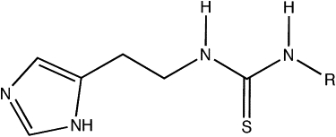
Scaffold of the thiourea-containing compounds. The R groups for the different compounds are displayed in Table 1.
Table 1.
The R-groups of the set of 12 thiourea-containing compounds used in the study
| Compound name | R | Structure |
|---|---|---|
| TH1 | Methyl | |
| TH2 | Ethyl | |
| TH3 | 1-Propyl | |
| TH4 | 2-Propyl | |
| TH5 | cHexyl |  |
| TH6 | Phenyl |  |
| TH7 | p-Methylphenyl |  |
| TH8 | p-Methoxyphenyl |  |
| TH9 | p-Chlorophenyl |  |
| TH10 | Methylphenyl |  |
| TH11 | Methyl-(p-methoxy)phenyl |  |
| TH12 | Ethylphenyl |  |
Figure 2.
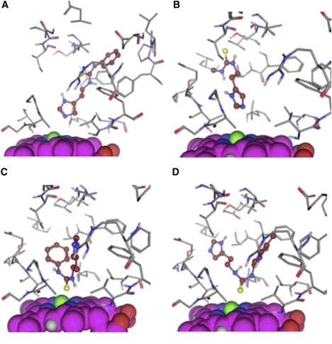
Examples of the four different starting conformations for the MD simulations. The heme is displayed in space-fill and is oriented in the same way in all figures. The ligand is displayed in ball-and-stick, with carbon atoms and the residues of the protein in sticks. (A) N_1 pose of compound TH6. (B) N_2 pose of compound TH1. (C) Pose S_1 of compound TH6. (D) Pose S_2 of compound TH7.
The structure of P450 2C9 cocrystallized with flurbiprofen, PDB code 1R9O (45), was used for the docking calculations and the following MD simulations. Missing loops in the crystal structure were modeled-in for the MD simulations, using MOE (46) and GROMOS05 (47). No crystallographic water molecules were included in the docking or the MD simulations. All docking calculations were performed with GOLD version 3.2 (48,49). Both the GOLDScore and the ChemScore (50) scoring functions were used to guide the docking and score the resulting docking poses. The radius of the sphere in which the docking program tries to position the ligand was set to 15 Å, centered in the middle of the active site. For the rest, default settings were used. Fifty docking poses of each scoring function were saved and visually inspected. Binding modes in accordance with N_1, N_2, S_1, or S_2, with the expected point of interaction close to and directed toward the heme-Fe, were selected for further MD simulation. The expected interaction points for all of the compounds were the Nɛ of the imidazole and the S atom of the thiourea group. For ligands where these poses did not appear in the top 50 poses of either GOLDScore or ChemScore, the pose was created by superposition on a similar compound displaying that particular pose followed by energy minimization or by restrained minimization, restraining the distance between the point of interaction and the heme-Fe.
Simulation settings
The thiourea-containing compounds were parameterized using the GROMOS force field, parameter set 45A4 (51), see Supporting Material for the parameterization of the scaffold. All setup, simulations, and analysis were performed with the GROMOS05 (47) and GROMACS 3.2.1 (52,53) biomolecular simulation packages. Protein simulations of 2 ns were performed for all the ligands and the ligand-surrounding interaction energies were inspected for convergence. The interaction energies of the final 1 ns were used for averaging and LIE model building and calculations. Pose N_1 was observed in the docking solutions of all the ligands, and extra simulations were performed for this pose starting from the same structure but using different random starting velocities. The ligands were also simulated free in solution for 1 ns.
The simulations were performed using the following protocol. The energy-minimized molecular structure was centered in a periodic truncated octahedron solvated with ∼16,700 (protein) and 1100 (free) simple-point charge water molecules (54). One Cl− counterion was added at a random position in the box of the protein simulation to obtain the same net charge of zero in the protein simulation as in the simulation of ligand free in solution. Initial velocities were randomly assigned according to a Maxwell-Boltzmann distribution at 50 K. The system was gradually heated up to 298 K, increasing the temperature by 50 K every 20 ps, followed by 40 ps of equilibration. During the heating up of the system, position restraints on the heavy atoms were gradually released. Subsequently, 2 ns of simulation was performed. For some of the systems, extended simulations were carried out, to reach convergence of the interaction energies. A time step of 2 fs was used and all bonds were constrained using the LINCS algorithm (55). The simulations were conducted at constant temperature and pressure, using the weak coupling algorithm (56). The solute and solvent molecules were separately coupled to two temperature baths at 298 K with a relaxation time of 0.1 ps. The relaxation time for the isotropic pressure scaling was set to 0.3 ps with an isothermal compressibility of 2.807 × 10⁻⁵ atm−1 and a reference pressure of 1 atm. Nonbonded interactions within 0.8 nm were calculated every time step using a pair list generated every fifth time-step. Long-range interactions, up to 1.4 nm, were calculated every fifth time-step. A reaction-field term was added to the energies and forces, with an effective dielectric constant of 61.0 to represent the electrostatic interactions outside the 1.4-nm cutoff (57). Solute coordinates were stored every 0.4 ps for the solute and energies were stored every 0.02 ps.
Results and Discussion
The GOLD and ChemScore docking scores are not free energies of binding and cannot be compared directly to the experimental values or the values calculated by the LIE method below. However, the ranking of the compounds based on the scores can be expressed in terms of the Spearman rank. The ranking of the compounds was unsatisfactory, displaying a Spearman rank of 0.30 for the docked N_1 poses, using ChemScore.
Throughout the simulations the protein structure remained well conserved with atom positional root mean-square (RMS) deviations with respect to the crystal structure of, at most, 0.3 nm for the backbone atoms. The inhibitors were relatively mobile in the active site, although interconversions of one pose to another during the simulations were not observed.
A classic LIE model, only including the N_1 docked conformations (see Fig. 2 A) as starting structures for the simulations, was constructed (Model 1). The last nanoseconds of the 2-ns simulations were used to calculate the energy averages. The resulting model is displayed in Fig. 3. The resulting LIE model has an RMS error of 5.4 kJ/mol (see Table 2), and displays four compounds for which the predictions deviate >6 kJ/mol. The Spearman rank is 0.52, an improvement compared to the docking scores, which corresponds to a reasonable ranking of the compounds.
Figure 3.
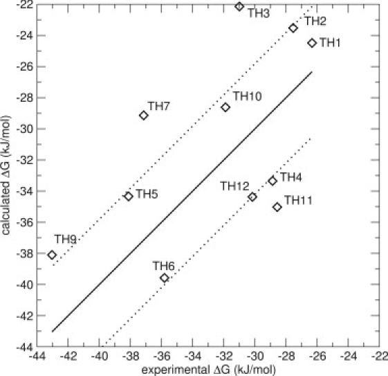
LIE Model 1 for the thiourea compounds, including energies from simulations of one docked pose (N_1). The thick line is not a correlation line, but indicates the perfect correlation between experimental and calculated values. The thin lines represent an error of ±4.19 kJ/mol (1 kcal/mol). The values are α = 0.53 and β = 0.11. The RMS error is 5.4 kJ/mol. The marker for compound TH8 falls outside the scale of the graph.
Table 2.
Summary of the results of the different LIE models
| LIE model No. | Starting structures | α | β | RMS error (kJ/mol) | Spearman rank |
|---|---|---|---|---|---|
| 1 | One pose (docked); N_1 | 0.53 | 0.11 | 5.4 | 0.52 |
| 2 | Four poses (docked and superposed); N_1, N_2, S_1, and S_2 | 0.50 | 0.11 | 4.7 | 0.52 |
| 3 | Three poses (docked); 3∗N_1 | 0.54 | 0.28 | 4.3 | 0.59 |
| 4 | One pose (restrained); N_1 | 0.53 | 0.11 | 5.3 | 0.52 |
| 5 | Three poses (restrained); N_1, N_2, and S_1 | 0.54 | 0.39 | 6.1 | 0.10 |
| 6 | Three poses (docked and superposed); N_1, N_2, and S_1 | 0.50 | 0.12 | 4.7 | 0.53 |
| 7 | Maximum four poses (only docked); N_1, N_2, S_1, and S_2 | 0.53 | 0.20 | 3.7 | 0.59 |
| 8 | Maximum six poses (only docked); N_1, N_2, S_1, and S_2 | 0.54 | 0.51 | 2.9 | 0.69 |
| 9 | One pose (selected from Model 8) | 0.54 | 0.51 | 3.0 | 0.61 |
Including multiple poses
Because of the lack of experimental information about binding modes of the thiourea-containing compounds in P450 2C9, and the large flexibility displayed by P450s, several different starting structures were used to try to improve the model. These conformations correspond to the binding modes displayed in Fig. 2, A–D. For most of the compounds it was not possible to find all the four different binding modes among the docking poses. These compounds were therefore superposed on a similar compound displaying that specific binding mode, followed by energy minimization. The energy averages from the four different simulations for each compound were combined according to Scheme 1. Varying the starting values of α and β did not change the new values of α and β significantly, indicating a robust method. Typically 5–10 iterations were needed to reach convergence of the values of α and β. The resulting model (Model 2) displays a slightly improved RMS error and the same Spearman rank compared to using only one pose. However, studying the relative weights, [i]A, for each conformation and compound, it is clear that for some of the compounds the additional simulations using different starting structures are relevant, leading to an improved model. As an example, compound TH3, an outlier with an error of 8.8 kJ/mol in Model 1, displays an error of −2.2 kJ/mol in Model 2, and the relative weights for this compound strongly favor another pose than the one used in Model 1, namely pose N_2. Model 2 displays four compounds with errors >6 kJ/mol, two of which are the same compounds as the outliers in Model 1, but with reduced errors and contributions from more poses. On the other hand, two compounds for which several poses are contributing show larger deviations from experimental values in Model 2 than in Model 1.
To investigate whether the improvement of the model is a result of additional sampling, two additional N_1 simulations in the protein were performed for all the compounds, starting with different randomly generated starting velocities. A model using energy averages from the three N_1 simulations was constructed using Scheme 1 (Model 3); see Table 2. The value of β increases significantly from 0.11 to 0.28, whereas α stays approximately the same. The RMS error of this model is slightly decreased compared to the previous models, 4.3 kJ/mol, and the Spearman rank increases somewhat, indicating a better ranking. Previous studies have shown that a good LIE model is able to make predictions within 1 kcal/mol (4.19 kJ/mol) of the experimental values (25,58). Model 3 displays one big outlier (>7.5 kJ/mol), compound TH3, which in Model 2 displayed a favorable weight on pose N_2, which is not taken into account in Model 3. Fig. 4 displays Model 3.
Figure 4.
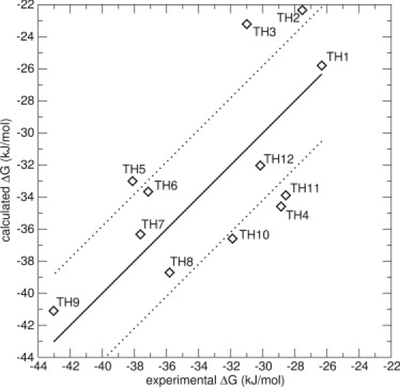
LIE Model 3 for the thiourea compounds, including energies from three simulations originating from one docked pose (N_1), but using different starting velocities. The thick line is not a correlation line, but indicates the perfect correlation between experimental and calculated values. The thin lines represent an error of ±4.19 kJ/mol (1 kcal/mol). The values are α = 0.54 and β = 0.28. The RMS error is 4.3 kJ/mol.
Effect of initial poses
The different docking poses that were selected were based on data of moieties coordinating the heme iron. Not all of the poses displayed the typical distance for atoms coordinating the heme-Fe, but were positioned slightly further away. To study whether a more pronounced coordination could reduce the errors in the previous models, three poses were positioned with the imidazole-Nɛ or the S of the thiourea moiety within ∼2.5 Å from the heme-Fe. The positioning was achieved by minimizing the complex using a distance restraint between the N or S and the Fe. Three different simulations starting from different starting conformations, corresponding to N_1, N_2, and S_1 (see Fig. 2, A–C), were performed. The LIE model originating from using only the restrained N_1 pose (Model 4) displays similar α and β values as by using the docked N_1 poses as starting structures, but displays larger errors (up to 10 kJ/mol) for three of the compounds. The RMS error is 5.3 kJ/mol. Including all the three poses results, similarly to including several simulations of N_1 docked poses, in a higher β of 0.39, whereas α stays approximately the same (Model 5). However, there are again three large outliers, different from the ones in Model 4, and the resulting RMS error is 6.1 kJ/mol, with a very poor Spearman rank of 0.10. This can be compared to Model 6, which includes the corresponding three docked poses, and which results in a better model with a RMS error of 4.7 kJ/mol, and Spearman rank of 0.53. Interestingly, these results indicate that it is more favorable to start simulations from docked poses similar to the expected binding mode, than starting from conformations that have been forced into the binding site, to strictly fulfill a certain hypothesis. The differences in the quality of the resulting models are significant.
Following the reasoning that it is more favorable to start simulations from docked poses, the model with four different docked poses (Model 2) was revised. As mentioned above, a representative of each of the four conformations for each compound was not always available in the docking poses. Therefore some starting structures were modeled by superposition on a similar molecule, followed by energy minimization. In Model 7, only docked poses have been included, which resulted in a varying amount of simulations for the different compounds, ranging from one to three. In this model, α and β are 0.53 and 0.20, respectively. All predictions are within 5.5 kJ/mol of the experimental values, the Spearman rank is improved to 0.59, and the RMS error is reduced to 3.7 kJ/mol. This again indicates that forcing the compounds in a specific pose may actually worsen the prediction and that the docking program is able to generate suitable starting positions, even if the scoring function does not correctly rank the different poses or the different compounds. It also indicates that in this particular case, the induced fit effect is not very large. Docking in a rigid structure followed by fully flexible MD simulations is sufficient to obtain improved affinity predictions.
Final model building
All the data, originating only from simulations of docked poses, were then included in one model, resulting in six possible conformations for each compound (Model 8). Respecting the criterion that only docked poses should be used, the data set resulted in a range of three-to-five energy averages for each compound. In this model, β increased to 0.51, very close to its theoretical value of 1/2, and α remained at a value of 0.54, very close to the α-values of the other models in Table 2. The fact that β increased to 0.51 in Model 8 is reassuring in the sense that it confirms the LIE theory. The RMS error decreased to 2.9 kJ/mol, unusually good for this type of calculation, and the Spearman rank increased to 0.69, which corresponds to a good ranking. Fig. 5 displays Model 8 and Table 3 displays the experimental and calculated values of this model. A Leave-One-Out cross validation was performed for Model 8. The resulting RMS error is 3.6 kJ/mol, which indicates a robust model.
Figure 5.
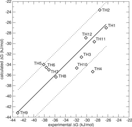
LIE Model 8 for the thiourea compounds, including energies from simulations of maximum six docked poses. The thick line is not a correlation line, but indicates the perfect correlation between experimental and calculated values. The thin lines represent an error of ±4.19 kJ/mol (1 kcal/mol). The values are α = 0.54 and β = 0.51. The RMS error is 2.9 kJ/mol. The only big outlier is compound TH4, with an error of 6.5 kJ/mol.
Table 3.
Experimental versus calculated free energies of binding for the best model, Model 8
| Compound | Experimental ΔG (kJ/mol)∗ | Calculated ΔG (kJ/mol)† | Error (kJ/mol) |
|---|---|---|---|
| TH1 | −26.3 | −27.0 | −0.7 |
| TH2 | −27.5 | −23.6 | 3.9 |
| TH3 | −31.0 | −32.6 | −1.6 |
| TH4 | −28.9 | −35.3 | −6.4 |
| TH5 | −38.1 | −34.0 | 4.1 |
| TH6 | −37.1 | −35.0 | 2.1 |
| TH7 | −37.6 | −34.5 | 3.1 |
| TH8 | −35.8 | −36.4 | −0.5 |
| TH9 | −43.0 | −43.2 | −0.2 |
| TH10 | −31.9 | −34.7 | −2.8 |
| TH11 | −28.6 | −29.7 | −1.1 |
| TH12 | −30.2 | −28.9 | 1.3 |
Compound TH4 is the only outlier, with an error of 6.5 kJ/mol. The matrix of the relative weights for the different conformations, [i]A, is shown in Table 4. As can be seen, it is mostly the simulations started from the N_1 conformation that contribute. The exceptions are compounds TH2, TH3, and TH8, where the N_2 conformation contributes significantly, as was observed in the previous models. For TH2 and TH8, multiple binding modes contribute similarly to the overall affinity. This may indicate that the loss of translational and rotational entropy upon ligand binding is different for these compounds, which may go against the implicit assumption in LIE that the entropy loss upon binding is similar for similar compounds. For compound TH7, the S_2 starting structure contributes the most. Interestingly, for the outlier TH4, there is only one docked pose taken into account in the calculations. The reason for this is that no other docking solutions, similar to the ones described in Fig. 2, were available. It is possible that, with the increased β-value of this model, the sampling of the TH4 compound is insufficient. Simulations using the starting structure S_1 do not contribute significantly for any of the compounds and could be left out, without significant changes to the model. This indicates that in a setup in which docking poses were not manually selected but all poses were included, the irrelevant poses will not affect the model.
Table 4.
Relative weights of the energies,, originating from the simulations with different starting structures, i, contributing to the total energy in Model 8
| Compound | Pose N_1 1 | Pose N_1 2 | Pose N_1 3 | Pose N_2 | Pose S_1 | Pose S_2 |
|---|---|---|---|---|---|---|
| TH1 | 0.0042 | 0.24 | 0.74 | 0.014 | —∗ | —∗ |
| TH2 | 0.17 | 0.23 | 0.054 | 0.54 | —∗ | —∗ |
| TH3 | 0† | 0.0025 | 0.011 | 0.98 | —∗ | —∗ |
| TH4 | 0.97 | 0.0067 | 0.025 | —∗ | —∗ | —∗ |
| TH5 | 0.17 | 0.80 | 0.035 | —∗ | —∗ | —∗ |
| TH6 | 0.0085 | 0.91 | 0.047 | —∗ | 0.034 | —∗ |
| TH7 | 0.017 | 0† | 0.0040 | —∗ | —∗ | 0.94 |
| TH8 | 0.0087 | 0.60 | 0.041 | 0.34 | 0.0098 | —∗ |
| TH9 | 0.11 | 0.54 | 0.35 | —∗ | —∗ | —∗ |
| TH10 | 0† | 0.95 | 0.0010 | —∗ | 0.048 | —∗ |
| TH11 | 0.57 | 0.022 | 0.41 | —∗ | —∗ | —∗ |
| TH12 | 0.41 | 0.026 | 0.56 | —∗ | —∗ | 0.0059 |
Conformation is not included in the energy calculation.
Relative weight <0.001.
One additional model, Model 9, was constructed using only the single most likely pose according to Table 4. A similar model is obtained with a RMS deviation error of 3.1 kJ/mol and a Spearman rank of 0.61. This shows that reasonable LIE models may be obtained using single simulations. The proposed method automatically selects the most appropriate pose from a number of suitable propositions from docking. For compounds TH2 and TH8, the predictions in Model 9 deteriorate slightly (deviations of 4.5 kJ/mol and 1.2 kJ/mol, respectively), because multiple binding modes, which are relevant for these compounds, are no longer included in Model 9.
It should be stressed that, even though our models seem able to include various poses, care should be taken to keep a balanced amount of poses for all the compounds, as α and β are intricately connected to the eventual relative weights of the poses. This was seen for compound TH4, an outlier in Model 8, where only one of the four different poses was sampled. That is, if insufficient poses, or poses with a very different balance between electrostatic and van der Waals energies are included for a compound, this will lead to variations of α and β, which subsequently leads to different relative weights of the poses.
In summary, we have introduced an iterative scheme that allows us to correctly include multiple independent MD simulations to obtain weighted ensemble averages to be used in the LIE formalism. This can be of importance for predictions in lead optimization programs if binding modes have not yet been determined experimentally. Nervall et al. (22) showed that the LIE method could distinguish between two distinct clusters of suggested docking poses of ligands in HIV reverse transcriptase. One of the clusters was close to a crystal structure conformation and considered to be correct. Scoring functions failed to predict the correct binding mode, whereas by using the optimized LIE parameters (27) the LIE model could predict the correct binding mode for each ligand in the set to have a more favorable free energy of binding. Our proposed scheme makes the initial pose selection less crucial for further simulation, as it automatically calculates the relative weights of the various poses. It also leaves the possibility open of multiple binding modes contributing similarly to the overall affinity, or of similar compounds occupying very different poses. It appears that the docking program is able to properly identify potential binding poses, even if the scoring function does not rank these appropriately. The proposed scheme weights the various poses based on thermodynamics and includes the information of all poses in the affinity prediction.
Conclusions
We have proposed a new iterative scheme that calculates weighted ensemble averages from multiple MD simulations to be used with the LIE method for binding affinity predictions. The accuracy of an initial, classic LIE model was significantly increased for a set of 12 thioureas binding to cytochrome P450 2C9. The best model displayed a RMS error of only 2.9 kJ/mol and was obtained by using all MD data starting from docked conformations. We also observed that using starting conformations from docking experiments leads to better models than using manually constructed or restrained starting poses. An increase in the overall sampling was seen to lead to an increased β-value, toward the theoretical value of 1/2.
Supporting Material
Force field parameters for the scaffold of the thiourea containing compounds are available at http://www.biophysj.org/biophysj/supplemental/S0006-3495(10)00310-3.
Supporting Material
Acknowledgments
We gratefully acknowledge financial support from The Netherlands Organization for Scientific Research (via Horizon Breakthrough grant No. 935-18-018 and VENI grant No. 700-55-401).
References
- 1.Moitessier N., Englebienne P., Corbeil C.R. Towards the development of universal, fast and highly accurate docking/scoring methods: a long way to go. Br. J. Pharmacol. 2008;153(Suppl 1):S7–S26. doi: 10.1038/sj.bjp.0707515. [DOI] [PMC free article] [PubMed] [Google Scholar]
- 2.Leach A.R., Shoichet B.K., Peishoff C.E. Prediction of protein-ligand interactions. Docking and scoring: successes and gaps. J. Med. Chem. 2006;49:5851–5855. doi: 10.1021/jm060999m. [DOI] [PubMed] [Google Scholar]
- 3.Warren G.L., Andrews C.W., Head M.S. A critical assessment of docking programs and scoring functions. J. Med. Chem. 2005;49:5912–5931. doi: 10.1021/jm050362n. [DOI] [PubMed] [Google Scholar]
- 4.Cheng T., Li X., Wang R. Comparative assessment of scoring functions on a diverse test set. J. Chem. Inf. Model. 2009;49:1079–1093. doi: 10.1021/ci9000053. [DOI] [PubMed] [Google Scholar]
- 5.Cross J.B., Thompson D.C., Humblet C. Comparison of several molecular docking programs: pose prediction and virtual screening accuracy. J. Chem. Inf. Model. 2009;49:1455–1474. doi: 10.1021/ci900056c. [DOI] [PubMed] [Google Scholar]
- 6.Ferrara P., Gohlke H., Brooks C.L. Assessing scoring functions for protein-ligand interactions. J. Med. Chem. 2004;47:3032–3047. doi: 10.1021/jm030489h. [DOI] [PubMed] [Google Scholar]
- 7.Stjernschantz E., Marelius J., Oostenbrink C. Are automated molecular dynamics simulations and binding free energy calculations realistic tools in lead optimization? An evaluation of the linear interaction energy (LIE) method. J. Chem. Inf. Model. 2006;46:1972–1983. doi: 10.1021/ci0601214. [DOI] [PubMed] [Google Scholar]
- 8.Claussen H., Buning C., Lengauer T. FlexE: efficient molecular docking considering protein structure variations. J. Mol. Biol. 2001;308:377–395. doi: 10.1006/jmbi.2001.4551. [DOI] [PubMed] [Google Scholar]
- 9.Sherman W., Day T., Farid R. Novel procedure for modeling ligand/receptor induced fit effects. J. Med. Chem. 2006;49:534–553. doi: 10.1021/jm050540c. [DOI] [PubMed] [Google Scholar]
- 10.Bottegoni G., Kufareva I., Abagyan R. A new method for ligand docking to flexible receptors by dual alanine scanning and refinement (SCARE) J. Comput. Aided Mol. Des. 2008;22:311–325. doi: 10.1007/s10822-008-9188-5. [DOI] [PMC free article] [PubMed] [Google Scholar]
- 11.Totrov M., Abagyan R. Flexible ligand docking to multiple receptor conformations: a practical alternative. Curr. Opin. Struct. Biol. 2008;18:178–184. doi: 10.1016/j.sbi.2008.01.004. [DOI] [PMC free article] [PubMed] [Google Scholar]
- 12.Rarey M., Kramer B., Lengauer T. The particle concept: placing discrete water molecules during protein-ligand docking predictions. Proteins. 1999;34:17–28. [PubMed] [Google Scholar]
- 13.Schnecke V., Kuhn L.A. Virtual screening with alvation and ligand-induced complementarity. Perspect. Drug Discov. Des. 2000;20:171–190. [Google Scholar]
- 14.Verdonk M.L., Chessari G., Taylor R. Modeling water molecules in protein-ligand docking using GOLD. J. Med. Chem. 2005;48:6504–6515. doi: 10.1021/jm050543p. [DOI] [PubMed] [Google Scholar]
- 15.Roberts B.C., Mancera R.L. Ligand-protein docking with water molecules. J. Chem. Inf. Model. 2008;48:397–408. doi: 10.1021/ci700285e. [DOI] [PubMed] [Google Scholar]
- 16.de Graaf C., Pospisil P., Vermeulen N.P. Binding mode prediction of cytochrome p450 and thymidine kinase protein-ligand complexes by consideration of water and rescoring in automated docking. J. Med. Chem. 2005;48:2308–2318. doi: 10.1021/jm049650u. [DOI] [PubMed] [Google Scholar]
- 17.Englebienne P., Moitessier N. Docking ligands into flexible and solvated macromolecules. 4. Are popular scoring functions accurate for this class of proteins? J. Chem. Inf. Model. 2009;49:1568–1580. doi: 10.1021/ci8004308. [DOI] [PubMed] [Google Scholar]
- 18.Vasanthanathan P., Hritz J., Oostenbrink C. Virtual screening and prediction of site of metabolism for cytochrome P450 1A2 ligands. J. Chem. Inf. Model. 2009;49:43–52. doi: 10.1021/ci800371f. [DOI] [PubMed] [Google Scholar]
- 19.Santos R., Hritz J., Oostenbrink C. Role of water in molecular docking simulations of cytochrome P450 2D6. J. Chem. Inf. Model. 2010;50:146–154. doi: 10.1021/ci900293e. [DOI] [PubMed] [Google Scholar]
- 20.Andér M., Luzhkov V.B., Aqvist J. Ligand binding to the voltage-gated Kv1.5 potassium channel in the open state—docking and computer simulations of a homology model. Biophys. J. 2008;94:820–831. doi: 10.1529/biophysj.107.112045. [DOI] [PMC free article] [PubMed] [Google Scholar]
- 21.Carlsson J., Boukharta L., Åqvist J. Combining docking, molecular dynamics and the linear interaction energy method to predict binding modes and affinities for non-nucleoside inhibitors to HIV-1 reverse transcriptase. J. Med. Chem. 2008;51:2648–2656. doi: 10.1021/jm7012198. [DOI] [PubMed] [Google Scholar]
- 22.Nervall M., Hanspers P., Aqvist J. Predicting binding modes from free energy calculations. J. Med. Chem. 2008;51:2657–2667. doi: 10.1021/jm701218j. [DOI] [PubMed] [Google Scholar]
- 23.Waszkowycz B. Towards improving compound selection in structure-based virtual screening. Drug Discov. Today. 2008;13:219–226. doi: 10.1016/j.drudis.2007.12.002. [DOI] [PubMed] [Google Scholar]
- 24.Åqvist J., Medina C., Samuelsson J.E. A new method for predicting binding affinity in computer-aided drug design. Protein Eng. 1994;7:385–391. doi: 10.1093/protein/7.3.385. [DOI] [PubMed] [Google Scholar]
- 25.Åqvist J., Luzhkov V.B., Brandsdal B.O. Ligand binding affinities from MD simulations. Acc. Chem. Res. 2002;35:358–365. doi: 10.1021/ar010014p. [DOI] [PubMed] [Google Scholar]
- 26.Hansson T., Marelius J., Åqvist J. Ligand binding affinity prediction by linear interaction energy methods. J. Comput. Aided Mol. Des. 1998;12:27–35. doi: 10.1023/a:1007930623000. [DOI] [PubMed] [Google Scholar]
- 27.Almlöf M., Brandsdal B.O., Åqvist J. Binding affinity prediction with different force fields: examination of the linear interaction energy method. J. Comput. Chem. 2004;25:1242–1254. doi: 10.1002/jcc.20047. [DOI] [PubMed] [Google Scholar]
- 28.Denisov I.G., Makris T.M., Schlichting I. Structure and chemistry of cytochrome P450. Chem. Rev. 2005;105:2253–2277. doi: 10.1021/cr0307143. [DOI] [PubMed] [Google Scholar]
- 29.Guengerich F.P. Cytochrome p450 and chemical toxicology. Chem. Res. Toxicol. 2008;21:70–83. doi: 10.1021/tx700079z. [DOI] [PubMed] [Google Scholar]
- 30.Ekroos M., Sjögren T. Structural basis for ligand promiscuity in cytochrome P450 3A4. Proc. Natl. Acad. Sci. USA. 2006;103:13682–13687. doi: 10.1073/pnas.0603236103. [DOI] [PMC free article] [PubMed] [Google Scholar]
- 31.Stjernschantz E., Vermeulen N.P.E., Oostenbrink C. Computational prediction of drug binding and rationalization of selectivity towards cytochromes P450. Expert Opin. Drug Metab. Toxicol. 2008;4:513–527. doi: 10.1517/17425255.4.5.513. [DOI] [PubMed] [Google Scholar]
- 32.Guengerich F.P. Mechanisms of cytochrome P450 substrate oxidation: MiniReview. J. Biochem. Mol. Toxicol. 2007;21:163–168. doi: 10.1002/jbt.20174. [DOI] [PubMed] [Google Scholar]
- 33.Isin E.M., Guengerich F.P. Kinetics and thermodynamics of ligand binding by cytochrome P450 3A4. J. Biol. Chem. 2006;281:9127–9136. doi: 10.1074/jbc.M511375200. [DOI] [PubMed] [Google Scholar]
- 34.Hritz J., de Ruiter A., Oostenbrink C. Impact of plasticity and flexibility on docking results for cytochrome P450 2D6: a combined approach of molecular dynamics and ligand docking. J. Med. Chem. 2008;51:7469–7477. doi: 10.1021/jm801005m. [DOI] [PubMed] [Google Scholar]
- 35.Zhou D., Afzelius L., Zamora I. Comparison of methods for the prediction of the metabolic sites for CYP3A4-mediated metabolic reactions. Drug Metab. Dispos. 2006;34:976–983. doi: 10.1124/dmd.105.008631. [DOI] [PubMed] [Google Scholar]
- 36.Chohan K.K., Paine S.W., Waters N.J. Quantitative structure activity relationships in drug metabolism. Curr. Top. Med. Chem. 2006;6:1569–1578. doi: 10.2174/156802606778108960. [DOI] [PubMed] [Google Scholar]
- 37.Arimoto R. Computational models for predicting interactions with cytochrome p450 enzyme. Curr. Top. Med. Chem. 2006;6:1609–1618. doi: 10.2174/156802606778108951. [DOI] [PubMed] [Google Scholar]
- 38.Onderwater, R. 2005. Molecular toxicology of thiourea-containing compounds. PhD thesis. Vrije Universiteit, Amsterdam.
- 39.Jarzynski C. Nonequilibrium equality for free energy differences. Phys. Rev. Lett. 1997;78:2690–2693. [Google Scholar]
- 40.Hritz J., Oostenbrink C. Efficient free energy calculations for compounds with multiple stable conformations separated by high energy barriers. J. Phys. Chem. B. 2009;113:12711–12720. doi: 10.1021/jp902968m. [DOI] [PubMed] [Google Scholar]
- 41.Testa B., Jenner P. Inhibitors of cytochrome P-450s and their mechanism of action. Drug Metab. Rev. 1981;12:1–117. doi: 10.3109/03602538109011082. [DOI] [PubMed] [Google Scholar]
- 42.Verras A., Kuntz I.D., Ortiz de Montellano P.R. Computer-assisted design of selective imidazole inhibitors for cytochrome p450 enzymes. J. Med. Chem. 2004;47:3572–3579. doi: 10.1021/jm030608t. [DOI] [PubMed] [Google Scholar]
- 43.Kayser H., Eilinger P. Metabolism of diafenthiuron by microsomal oxidation: procide activation and inactivation as mechanisms contributing to selectivity. Pest Manag. Sci. 2001;57:975–980. doi: 10.1002/ps.360. [DOI] [PubMed] [Google Scholar]
- 44.Stevens G.J., Hitchcock K., Mangold B.L. In vitro metabolism of N-(5-chloro-2-methylphenyl)-N′-(2-methylpropyl)thiourea: species comparison and identification of a novel thiocarbamide-glutathione adduct. Chem. Res. Toxicol. 1997;10:733–741. doi: 10.1021/tx9700230. [DOI] [PubMed] [Google Scholar]
- 45.Wester M.R., Yano J.K., Johnson E.F. The structure of human cytochrome P450 2C9 complexed with flurbiprofen at 2.0-Å resolution. J. Biol. Chem. 2004;279:35630–35637. doi: 10.1074/jbc.M405427200. [DOI] [PubMed] [Google Scholar]
- 46.Chemical Computing Group. MOE: Molecular Operating Environment. C.C.G. Inc., Montreal, Quebec, Canada.
- 47.Christen M., Hünenberger P.H., Van Gunsteren W.F. The GROMOS software for biomolecular simulation: GROMOS05. J. Comput. Chem. 2005;26:1719–1751. doi: 10.1002/jcc.20303. [DOI] [PubMed] [Google Scholar]
- 48.Jones G., Willett P., Glen R.C. Molecular recognition of receptor sites using a genetic algorithm with a description of desolvation. J. Mol. Biol. 1995;245:43–53. doi: 10.1016/s0022-2836(95)80037-9. [DOI] [PubMed] [Google Scholar]
- 49.Jones G., Willett P., Taylor R. Development and validation of a genetic algorithm for flexible docking. J. Mol. Biol. 1997;267:727–748. doi: 10.1006/jmbi.1996.0897. [DOI] [PubMed] [Google Scholar]
- 50.Eldridge M.D., Murray C.W., Mee R.P. Empirical scoring functions: I. The development of a fast empirical scoring function to estimate the binding affinity of ligands in receptor complexes. J. Comput. Aided Mol. Des. 1997;11:425–445. doi: 10.1023/a:1007996124545. [DOI] [PubMed] [Google Scholar]
- 51.Schuler L.D., Daura X., van Gunsteren W.F. An improved GROMOS96 force field for aliphatic hydrocarbons in the condensed phase. J. Comput. Chem. 2001;22:1205–1218. [Google Scholar]
- 52.Berendsen H.J.C., Van der Spoel D., Van Drunen R. GROMACS: a message-passing parallel molecular dynamics implementation. Comput. Phys. Commun. 1995;91:43–56. [Google Scholar]
- 53.Lindahl E., Hess B., Van der Spoel D. GROMACS 3.0: a package for molecular simulation and trajectory analysis. J. Mol. Model. 2001;7:306–317. [Google Scholar]
- 54.Berendsen H.J.C., Postma J.P.M., Hermans J. Intermolecular Forces. Reidel; Dordrecht, The Netherlands: 1981. Interaction models for water in relation to protein hydration. [Google Scholar]
- 55.Hess B., Bekker H., Fraaije J.G.E.M. LINCS: a linear constraint solver for molecular simulations. J. Comput. Chem. 1997;18:1463–1472. [Google Scholar]
- 56.Berendsen H.J.C., Postma J.P.M., Haak J.R. Molecular-dynamics with coupling to an external bath. J. Chem. Phys. 1984;81:3684–3690. [Google Scholar]
- 57.Tironi I.G., Sperb R., van Gunsteren W.F. A generalized reaction field method for molecular-dynamics simulations. J. Chem. Phys. 1995;102:5451–5459. [Google Scholar]
- 58.Brandsdal B.O., Österberg F., Aqvist J. Free energy calculations and ligand binding. Adv. Protein Chem. 2003;66:123–158. doi: 10.1016/s0065-3233(03)66004-3. [DOI] [PubMed] [Google Scholar]
Associated Data
This section collects any data citations, data availability statements, or supplementary materials included in this article.