TEAM: efficient two-locus epistasis tests in human genome-wide association study

Abstract

As a promising tool for identifying genetic markers underlying phenotypic differences, genome-wide association study (GWAS) has been extensively investigated in recent years. In GWAS, detecting epistasis (or gene–gene interaction) is preferable over single locus study since many diseases are known to be complex traits. A brute force search is infeasible for epistasis detection in the genome-wide scale because of the intensive computational burden. Existing epistasis detection algorithms are designed for dataset consisting of homozygous markers and small sample size. In human study, however, the genotype may be heterozygous, and number of individuals can be up to thousands. Thus, existing methods are not readily applicable to human datasets. In this article, we propose an efficient algorithm, TEAM, which significantly speeds up epistasis detection for human GWAS. Our algorithm is exhaustive, i.e. it does not ignore any epistatic interaction. Utilizing the minimum spanning tree structure, the algorithm incrementally updates the contingency tables for epistatic tests without scanning all individuals. Our algorithm has broader applicability and is more efficient than existing methods for large sample study. It supports any statistical test that is based on contingency tables, and enables both family-wise error rate and false discovery rate controlling. Extensive experiments show that our algorithm only needs to examine a small portion of the individuals to update the contingency tables, and it achieves at least an order of magnitude speed up over the brute force approach.

Contact: xiang@cs.unc.edu

1 INTRODUCTION

Genetic association analysis examines the statistical correlation between an organism's genotype with its phenotype. With the development of high-throughput genotyping technologies, genetic variation of human and other model organisms has been measured at genome-wide scale. As the most abundant source of genetic variation, the number of single nucleotide polymorphism (SNPs) in public databases (dbGaP, JAX) is up to millions. Genome-wide association study (GWAS) has been shown to be a promising tool to locate the genetic factors that cause phenotypic differences (Saxena et al., 2007; Scuteri et al., 2007; WTCCC, 2007; Weedon et al., 2007). Epistasis, or gene–gene interaction detection, has received increasing attention in complex trait analysis. Different from single-locus approach, the goal of two-locus epistasis detection is to identify interacting SNP pairs that have strong association with the phenotype. Please refer to Balding (2006), Hirschhorn and Daly (2005), Hoh and Ott (2003) and Musani et al. (2007) for reviews of current progress and challenges in epistasis detection in GWAS.

There are two grand challenges in epistasis detection. The first is to develop statistical tests that can effectively capture the interaction between SNPs. Various tests have been proposed for two-locus association study, such as the chi-square test, likelihood ratio test and entropy-based test (Balding, 2006). Another crucial challenge in two-locus association study is the intensive computational burden imposed by the enormous search space. Suppose that there are N SNPs for M individuals. The overall search space of pairwise interactions is MN(N − 1)/2. The large number of tests also causes the multiple testing problem (Miller, 1981). Controlling the family-wise error rate (FWER) and false discovery rate (FDR) are standard ways to control the error rate (Dudoit and Laan, 2008; Westfall and Young, 1993). In the FWER and FDR controlling, permutation test is preferred over simple Bonferroni correction since many SNPs are correlated (Churchill and Doerge, 1994). The correlation structure among genotype profiles is preserved across permutations and is incorporated into permutation P-value estimation. The idea of permutation test is to randomly shuffle the phenotype values among the individuals and recalculate the test statistics. The distribution of these test values are used to estimate the null distribution. Permutation test dramatically increases the search space. With K permutations, the entire search space of two-locus association mapping is KMN(N − 1)/2. Consider a moderate GWAS setting, in which M = 1000, N = 100 000 and K = 1000. The size of the search space is about 5 × 10¹⁵. Apparently, a brute force enumeration of the search space is infeasible and thus efficient algorithms are in demand.

Although the computational challenge of epistasis detection has been well recognized, the algorithmic development is still very limited. For a small number of SNPs, e.g. from tens to a few hundreds, exhaustive algorithms that explicitly enumerate all possible SNP combinations have been developed (Nelson et al., 2001; Ritchie et al., 2001). These methods are not scalable for genome-wide computing. Genetic algorithm (Carlborg et al., 2000) has been proposed. This approach is heuristic, which does not guarantee to find the optimal solution. To avoid explicitly exploring the entire search space, a common heuristic used in epistasis detection is a two-step approach (Evans et al., 2006; Hoh et al., 2000; Yang et al., 2009). First, a subset of SNPs are selected according to certain criteria. Then the selected SNPs are used for subsequent epistatic analysis. However, the SNP screening process suffers from the same problem as the single-locus approach. SNPs with strong epistasis but low marginal effects are likely to be filtered out (Zhang et al., 2009a).

Recently, the approach based on search space pruning has been shown to be able to dramatically speed up the process of epistasis detection without compromising the optimality of the results. FastANOVA (Zhang et al., 2008) and FastChi (Zhang et al., 2009b) are specifically designed for ANOVA test and chi-square test, respectively. The COE algorithm (Zhang et al., 2009a) is a more general approach that is applicable to all convex tests. Utilizing an upper bound derived for the test being used, these algorithms only need to examine a small number of promising SNP pairs and prune the SNP pairs that are proven to have no strong association with the phenotype. Unlike heuristic approaches, these algorithms are guaranteed to find the optimal solution. Although these methods provide promising alternatives for GWAS, there are two major drawbacks that limit their applicability. First, they are designed for relatively small sample size and only consider homozygous markers (i.e. each SNP can be represented as a {0, 1} binary variable). In human study, however, the sample size is usually large and most SNPs contain heterozygous genotypes and are coded using {0, 1, 2}. These make existing methods intractable. Second, although the FWER and the FDR are both widely used for error controlling, existing methods are designed only to control the FWER. From a computational point of view, the difference in the FWER and the FDR controlling is that, to estimate FWER, for each permutation, only the maximum two-locus test value is needed. To estimate the FDR, on the other hand, for each permutation, all two-locus test values must be computed. Further details of the FWER and the FDR controlling are described in Section 2.

In this article, we propose an exhaustive algorithm, TEAM (Tree-based Epistasis Association Mapping), for efficient epistasis detection in human GWAS. TEAM has several advantages over previous methods.

• It supports to both homozygous and heterozygous data.

• By exhaustively computing all two-locus test values in permutation test, it enables both FWER and FDR controlling.

• It is applicable to all statistics based on the contingency table. Previous methods are either designed for specific tests or require the test statistics to satisfy certain property.

• Experimental results demonstrate that TEAM is more efficient than existing methods for large sample study.

TEAM incorporates permutation test for proper error controlling. The key idea is to incrementally update the contingency tables of two-locus tests. We show that only four of the 18 observed frequencies in the contingency table need to be updated to compute the test value. In the algorithm, we build a minimum spanning tree (Cormen et al., 2001) on the SNPs. The nodes of the tree are SNPs. Each edge represents the genotype difference between the two connected SNPs. This tree structure can be utilized to speed up updating process for the contingency tables. A majority of the individuals are pruned and only a small portion are scanned to update the contingency tables. This is advantageous in human study, which usually involves thousands of individuals. Extensive experimental results demonstrate the efficiency of the TEAM algorithm.

2 THE PROBLEM OF TWO-LOCUS EPISTASIS DETECTION IN HUMAN GWAS

Suppose that the genotype dataset consists of N SNPs {X₁,…, X_N} for M individuals {S₁,…, S_M}. We adopt the convention of using 0 and 2 to represent the homozygous majority and homozygous minority genotypes, respectively, and 1 to represent the heterozygous case. Let Y₀ ∈ {0, 1} be the phenotype of interest (0 for controls and 1 for cases). Let Y′ = {Y₁,…, Y_K} be the set of K permutations of Y₀. In each permutation Y_k, the phenotype labels are randomly reassigned to individuals with no replacement.

Table 1 shows an example dataset of SNPs and phenotype permutations. The genotype dataset consists of six SNPs {X₁,…, X₆} for 24 individuals {S₁,…, S₂₄}. Individuals {S₁,…, S₁₂} are cases and {S₁₃,…, S₂₄} are controls. The phenotype is permuted five times, i.e. Y′ = {Y₁,…, Y₅}.

Table 1.

An example dataset consisting of six SNPs {X₁,…, X₆}, the original phenotype Y₀ and five phenotype permutations {Y₁,…, Y₅} for 24 individuals {S₁,…, S₂₄}

	S1	S2	S3	S4	S5	S6	S7	S8	S9	S10	S11	S12	S13	S14	S15	S16	S17	S18	S19	S20	S21	S22	S23	S24
X1	0	0	0	1	2	0	2	0	2	0	0	2	0	0	0	2	0	2	1	0	0	2	2	0
X2	2	2	0	2	0	2	0	2	2	2	2	0	1	0	0	2	0	2	1	0	2	2	2	2
X3	2	0	0	2	0	2	0	1	2	1	2	2	1	0	2	2	0	2	1	2	2	2	2	2
X4	0	2	2	0	0	0	2	1	0	2	2	0	0	0	0	0	0	0	1	0	1	2	0	0
X5	0	2	2	0	0	0	1	1	2	1	2	0	0	0	0	0	0	2	1	0	2	2	0	2
X6	0	2	2	0	0	0	2	1	0	1	2	0	0	0	0	2	0	2	1	0	2	2	0	0
Y0	1	1	1	1	1	1	1	1	1	1	1	1	0	0	0	0	0	0	0	0	0	0	0	0
Y1	0	1	0	0	1	1	1	0	0	0	1	1	1	1	1	0	1	0	0	1	0	1	0	0
Y2	0	0	1	0	1	1	1	1	1	1	0	0	1	0	0	1	1	1	0	0	0	1	0	0
Y3	1	0	1	1	1	1	0	1	1	1	0	0	0	1	0	1	0	0	1	0	0	0	1	0
Y4	0	1	1	1	1	1	0	0	0	1	0	0	1	0	1	0	0	0	1	1	0	1	1	0
Y5	1	0	1	1	0	0	0	0	0	1	1	1	1	0	1	1	0	0	0	0	0	1	1	1

Let ℑ denote the statistical test to be used. Specifically, we represent the test value of SNP X_i and phenotype Y_k (0≤k≤K) as ℑ(X_i, Y_k), and represent the test value of SNP pair (X_iX_j) and Y_k as ℑ(X_iX_j, Y_k). A contingency table that records the observed values of certain events, is the basis of many statistical tests. Tables 2–4 show contingency tables for the single-locus tests ℑ(X_i, Y_k) and ℑ(X_j, Y_k), genotype relationship between SNPs X_i and X_j and two-locus test ℑ(X_iX_j, Y_k), respectively.

Table 2.

Contingency tables for single-locus tests ℑ(X_i, Y_k) and ℑ(X_j, Y_k)

Contingency table for ℑ(Xi, Yk)					Contingency table for ℑ(Xj, Yk)
	Xi=0	Xi=1	Xi=2	Total		Xj=0	Xj=1	Xj=2	Total
Yk=0	Event A	Event B	Event E		Yk=0	Event G	Event H	Event I
Yk=1	Event C	Event D	Event F		Yk=1	Event J	Event L	Event O
Total				M	Total				M

Table 3.

Contingency table for genotype relation between two SNPs X_i and X_j

	Xi=0	Xi=1	Xi=2	Total
Xj=0	Event S	Event T	Event R
Xj=1	Event P	Event Q	Event U
Xj=2	Event V	Event W	Event Z
Total				M

Table 4.

Contingency table for two-locus test ℑ(X_iX_j, Y_k)

	Xi=0			Xi=1			Xi=2			Total
	Xj=0	Xj=1	Xj=2	Xj=0	Xj=1	Xj=2	Xj=0	Xj=1	Xj=2
Yk=0	Event a1	Event a2	Event a3	Event b1	Event b2	Event b3	Event e1	Event e2	Event e3
Yk=1	Event c1	Event c2	Event c3	Event d1	Event d2	Event d3	Event f1	Event f2	Event f3
Total										M

Due to the large number of hypotheses being tested, multiple testing problem has received considerable attention in GWAS. Controlling the FWER and FDR are two widely used approaches to control the error rate. The FWER is the probability of having at least one false positive. The FDR is the expected proportion of false positives among rejected hypotheses. Permutation test is the standard way to estimate the null distribution in both approaches. Next, we briefly describe the typical procedures of the FWER and FDR control. For statistical background of these approaches, refer to Dudoit and Laan (2008) and Westfall and Young (1993) for details.

The FWER controlling procedure: for each permutation Y_k ∈ Y′, let ℑ_Yk represent the maximum test value among all SNP pairs, i.e. ℑ_Yk = max {ℑ(X_iX_j, Y_k)|1 ≤ i < j ≤ N}. The distribution of {ℑ_Yk|Y_k ∈ Y′} is used as the null distribution. Given an error rate threshold α, the critical value ℑ_α is the αK-th largest value in {ℑ_Yk|Y_k ∈ Y′}. A SNP pair (X_iX_j) is considered significant if its test value with the original phenotype Y₀ exceeds the critical value, i.e. ℑ₍X_iX_j, Y₀)≥ℑ_α.

The FDR controlling procedure: let PV represent the set of the pooled test values of all permutation tests, i.e. PV={ℑ(X_iX_j, Y_k)|1≤i<j≤N, 1≤k≤K}. The P−value of test ℑ(X_iX_j, Y₀) can be calculated as p(ℑ(X_iX_j, Y₀))=|{t≥ℑ(X_iX_j, Y₀)|t∈PV}|/|PV|, i.e. the proportion of the values in PV that are no less than ℑ(X_iX_j, Y₀). Let p₍₁₎≤p₍₂₎…≤p_(N(N−1)/2) be the ordered P-values of the original tests. Let . The classic Benjamini–Hochberg method rejects all hypotheses for which the corresponding P-values are in the set {p₍₁₎, p₍₂₎,…, p_(v)}.

In the FWER controlling, we only need the maximum test value of each permutation. To control the FDR, all test values need to be computed to estimate the P-value of the original tests. The existing algorithms, such as FastChi (Zhang et al., 2009b) and COE (Zhang et al., 2009a), prune the SNP pairs having weak associations. Thus they cannot be used to control the FDR. Our algorithm, TEAM, exhaustively computes the test values of all SNP pairs for every permutation. It can be used for both the FWER and FDR controlling. In this article, we mainly focus on the problem of permutation test, since it is the most computationally intensive procedure. Testing SNP pairs using original phenotype can be treated as a special case of permutation test.

3 FREE VARIABLES IN THE CONTINGENCY TABLE OF TWO-LOCUS TEST

Let E_event and O_event denote the expected frequency and observed frequency of an event in Tables 2–4. Note that each event represents a subset of individuals. For example, event D is a subset of individuals satisfying (X_i = 1 ∧ Y_k = 1), and O_D represents its observed frequency, i.e. O_D = |D|. Using the dataset in Table 1, consider X₃ and Y₄ (i.e. i = 3 and k = 4), we have D = {S₁₀, S₁₃, S₁₉}, and O_D = 3.

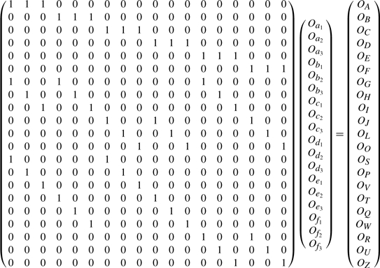
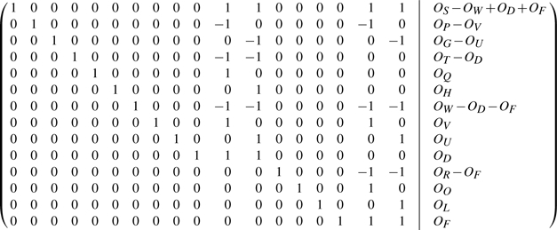
Many statistics, such as chi-square test and likelihood ratio test are defined as functions of the observed frequencies in contingency tables. For any test ℑ based on the contingency table, to calculate the two-locus test value ℑ(X_iX_j, Y_k), one needs all 18 observed frequencies for the events in the two-locus contingency table shown in Table 4. The following theorem shows that we only need four of the 18 values to calculate the two-locus test value given the three contingency tables in Tables 2 and 3.

Theorem 3.1. —

For SNPs X_i, X_j and permutation Y_k, given the observed frequencies in Tables 2 and 3, specifically, the values of {O_D, O_F, O_J, O_L, O_O, O_S, O_P, O_V, O_T, O_Q, O_W, O_R, O_U, O_Z}, all of the observed frequencies in Table 4 can be determined if the values of {O_d2, O_d3, O_f2, O_f3} are known.

Proof. —

See Appendix.

Suppose that we have all the single-locus contingency tables, i.e. Table 2. Given a SNP pair (X_i, X_j), Table 3 is fixed. Thus, from Theorem 3.1, for permutation Y_k, once we have the values of {O_d2, O_d3, O_f2, O_f3}, ℑ(X_iX_j, Y_k) can be calculated accordingly. In the following, we show that these values can be computed incrementally utilizing a minimum spanning tree built on SNPs. We focus on the incremental process for O_d2. The same process can be applied to update O_d3, O_f2 and O_f3. We first discuss how to update O_d2 for a specific permutation. Then we show that the procedure can also handle all the permutations in a batch mode.

4 BUILDING THE MINIMUM SPANNING TREE ON THE SNPS

To build a minimum spanning tree (Cormen et al., 2001) on the SNPs, let the SNPs {X₁, X₂,…, X_N} be the nodes and SNP pairs (X_iX_j) (i≠j) be the (undirected) edges. For each edge (X_iX_j), we denote its weight (the number of individuals having different genotypes in the two SNPs) as w(X_iX_j). A spanning tree 𝒯 is a tree that spans (connects) all SNPs. Let V(𝒯) be its node set and E(𝒯) be its edge set. A minimum spanning tree is a spanning tree whose weight W_𝒯=∑w(X_iX_j), where (X_iX_j) ∈ E(𝒯), is no greater than any other spanning tree. Figure 1 shows the minimum spanning tree built using the example dataset in Table 1. The number on each edge represents its weight. For example, in X₃ and X₂, there are six individuals, {S₂, S₈, S₁₀, S₁₂, S₁₅, S₂₀}, having different genotypes.

Fig. 1.

The minimum spanning tree built on the SNPs in the example dataset shown in Table 1.

For any individual, the genotype difference from X_i to X_j can be any one of the six combinations, i.e. 0→ 1 (indicating that the genotype in X_i is 0, and the genotype in X_j is 1), 1→ 0, 0→ 2, 2→ 0, 1→ 2 and 2→ 1. Using the example dataset in Table 1, Table 5 shows the genotype differences between the connected two SNPs in the minimum spanning tree in Figure 1. We use (X_iX_j)_{u→v}(u, v ∈ {0, 1, 2}) to represent the set of individuals whose genotype in X_i is u and genotype in X_j is v. For example, (X₃X₂)_{1→2}={S₈, S₁₀} and (X₃X₂)_{{1→2}∪{0→2}} = {S₂, S₈, S₁₀}.

Table 5.

Genotype difference between the connected SNPs in the minimum spanning tree shown in Figure 1

	0→1	1→0	0→2	2→0	1→2	2→1
(X3X2)	∅	∅	{S2}	{S12, S15, S20}	{S8, S10}	∅
(X2X5)	{S7}	{S13}	{S3}	{S1, S4, S6, S16, S23}	∅	{S8, S10}
(X5X6)	∅	∅	{S16}	{S9, S24}	{S7}	∅
(X6X1)	{S4}	{S8, S10}	{S5, S9, S12, S23}	{S2, S3, S11, S21}	∅	∅
(X6X4)	∅	∅	∅	{S16, S18}	{S10}	{S21}

5 INCREMENTALLY UPDATING OBSERVED FREQUENCY O_d2

In this section, we discuss how to update O_d2 by utilizing the minimum spanning tree. For clarity, from now on, we use d₂(X_iX_j, Y_k) to denote the specific event d₂ for the SNP pair (X_iX_j) and permutation Y_k, i.e. the subsets of individuals satisfying (X_i = 1 ∧ X_j = 1 ∧ Y_k=1). We use O_d2(X_iX_j, Y_k) to represent its observed frequency, i.e. O_d2(X_iX_j, Y_k)=|d₂(X_iX_j, Y_k)|. This notation also applies to other events in the contingency tables shown in Tables 2–4. For example, D(X_i, Y_k) represents the subset of individuals satisfying (X_i = 1 ∧ Y_k=1), and O_D(X_i, Y_k) = |D(X_i, Y_k)|.

Next, we show that for any SNP pair (X_iX_j) and an edge (X_jX_j′) ∈ E(𝒯), given O_d2(X_iX_j, Y_k), how to update the value for O_d2(X_iX_j′, Y_k). From the contingency tables in Table 2–4, it is easy to see that

and

The following theorem shows that, given O_d2(X_iX_j, Y_k) and D(X_i, Y_k), using the genotype difference associated with edge (X_jX_j′), we can get the value of O_d2(X_iX_j′, Y_k).

Theorem 5.1. —

For any SNP pair (X_iX_j) and an edge (X_jX_j′) ∈ E(𝒯), we have O_d2(X_iX_j′, Y_k) = O_d2(X_iX_j, Y_k)+|D(X_i, Y_k)∩(X_jX_j′)_{{0→1}∪{2→1}}|− |D(X_i, Y_k)∩(X_jX_j′)_{{1→0}∪{1→2}}|.

Proof. —

See Appendix.

Example 5.2. —

Using the example dataset in Table 1, let i=3, j=2, j′=5, and k=4, i.e. we consider SNP pair (X₃X₂), permutation Y₄ and the edge (X₂X₅) in Figure 1. Suppose that we already know that O_d2(X₃X₂, Y₄)=2, and event D(X₃, Y₄)={S₁₀, S₁₃, S₁₉}. From Table 5, we have (X₂X₅)_{{0→1}∪{2→1}}={S₇, S₈, S₁₀}, and (X₂X₅)_{{1→0}∪{1→2}}={S₁₃}. Thus according to Theorem 5.1, we have O_d2(X₃X₅, Y₄)=O_d2(X₃X₂, Y₄)+|{S₁₀}|−|{S₁₃}|=2. Note that by this way, we get the value of O_d2(X₃X₅, Y₄) from O_d2(X₃X₂, Y₄)without scanning all individuals.

So far, we have discussed the procedure to update the value of O_d2(X_iX_j′, Y_k) from O_d2(X_iX_j, Y_k) for a specific phenotype permutation Y_k. This procedure can be easily extended to handle all the permutations. From Theorem 5.1, for any permutation Y_k, to update the value of O_d2(X_iX_j′, Y_k) from O_d2(X_iX_j, Y_k), we need the value of D(X_i, Y_k) and the genotype difference associated with edge (X_jX_j′). Note that the genotype difference is fixed once the minimum spanning tree is built. Next, we discuss how to compute D(X_i, Y_k) for all permutations {Y₁, Y₂,…, Y_K} in a batch mode in detail.

Let D_K(X_i) be a list of M entries, with each entry corresponding to an individual. For each individual S_m, we record in D_K(X_i)[m] the set of phenotypes satisfying (X_i = 1 ∧ Y_k=1). For example, consider the dataset in Table 1, we have that D_K(X₃)[8]={Y₂, Y₃}. Table 4 shows the entries of D_K(X₃). Only non-empty entries, i.e. D_K(X_i)[m]≠∅, are shown in the table. It is easy to see that, for any X_i and Y_k, we can get D(X_i, Y_k) from D_K(X_i) as follows: D(X_i, Y_k) is the set of individuals whose corresponding entries in D_K(X_i) contain Y_k as an element, i.e.

(1)

For example, using the example dataset in Table 1, from Table 6, we know that D(X₃, Y₄)={S₁₀, S₁₃, S₁₉}.

Table 6.

Entries of D_K(X₃) with empty entries omitted for all permutations in a batch mode

Individual id.	Phenotype permutations
S8	{Y2, Y3}
S10	{Y2, Y3, Y4, Y5}
S13	{Y1, Y2, Y4, Y5}
S19	{Y3, Y4}

For SNP pair (X_iX_j), let O_d2(X_iX_j)=[O_d2(X_iX_j, Y₁), O_d2(X_iX_j, Y₂),…, O_d2(X_iX_j, Y_K)]. From Theorem 5.1 and Equation (1), for any SNP pair (X_iX_j) and an edge (X_jX_j′)∈E(𝒯), we can get O_d2(X_iX_j′) from O_d2(X_iX_j) using D_K(X_i) and the genotype difference information associated with edge (X_jX_j′). First, initialize O_d2(X_iX_j′)=O_d2(X_iX_j). Next, for every m (1≤m≤M), if Y_k ∈ D_K(X_i)[m], we update O_d2(X_iX_j′) as follows:

Example 5.3. —

Following Example 5.2, we consider the two SNP pairs (X₃X₂) and (X₃X₅), with (X₂X₅) being an edge of the tree in Figure 1. Assume that D_K(X₃) is as shown in Table 6, and O_d2(X₃X₂)=[1, 1, 1, 2, 1]. From Table 5, the genotype difference on edge (X₂X₅) is (X₂X₅)_{{0→1}∪{2→1}}={S₇, S₈, S₁₀}, and (X₂X₅)_{{1→0}∪{1→2}}={S₁₃}. For individual S_m ∈ {S₇, S₈, S₁₀} (S_m ∈ {S₁₃}), we need to increase (decrease) the corresponding values in O_d2(X₃X₂) according to D_K(X₃). Table 7 shows the updating process for O_d2(X₃X₅). Initially, O_d2(X₃X₅)=O_d2(X₃X₂). For individual S₇, since its corresponding entry in D_K(X3), D_K(X3)[7]=∅, O_d2(X₃X₅) remains unchanged. For individual S₈, D_K(X3)[8]={Y₂, Y₃}, we increase the values of O_d2(X₃X₅, Y₂) and O_d2(X₃X₅, Y₃) by 1. Similarly, we increase and decrease the values in O_d2(X₃X₅) according to D_K(X3) for S₁₀ and S₁₃. For individual S₁₉, we do not have any update because S₁₉ ∉ {S₇, S₈, S₁₀} and S₁₉ ∉ {S₁₃}. The final result is O_d2(X₃X₅)=[0, 2, 3, 2, 1].

Table 7.

Updating O_d2(X₃X₅) from O_d2(X₃X₂) for all permutations in a batch mode

	Y1	Y2	Y3	Y4	Y5
Od2(X3X5) after initializing	1	1	1	2	1
Od2(X3X5) after updating for S7	1	1	1	2	1
Od2(X3X5) after updating for S8	1	2	2	2	1
Od2(X3X5) after updating for S10	1	3	3	3	2
Od2(X3X5) after updating for S13	0	2	3	2	1

Note that to get the value of O_d2(X_iX_j), using a brute force approach, we need to scan a (2+K) × M matrix consisting of the genotype of (X_iX_j) and permutations {Y₁, Y₂,…, Y_K} for the M individuals. In the previous example, to compute the value of O_d2(X₃X₅), the cost of the brute force approach is (3+5) × 24=192. Using our approach, the total number of updates is |D_K(X3)[8]|+|D_K(X3)[10]|+|D_K(X3)[13]|=10, which is significantly less than the cost of the brute force approach. More formally, given D_K(X_i), the time complexity of updating O_d2(X_iX_j′) from O_d2(X_iX_j) is O(w(X_jX_j′)K).

The procedure of updating O_d2(X_iX_j′) from O_d2(X_iX_j) can also be applied to update the remaining free variables O_d3(X_iX_j), O_f2(X_iX_j) and O_f3(X_iX_j). Note that, to update O_f2(X_iX_j), O_f3(X_iX_j), we will need F_K(X_i), which can be defined in a similar way to that of D_K(X_i): for each individual S_m, we record in F_K(X_i)[m] the set of phenotypes satisfying (X_i = 2 ∧ Y_k=1).

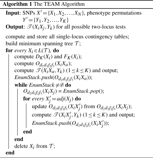
6 THE TEAM ALGORITHM

TEAM examines SNP pairs through a double loop, where the outer loop visits a leaf node at a time, and the inner loop traverse the rest of the tree, starting from the parent node of the leaf. Let O_d2d3f2f3(X_iX_j)=[O_d2(X_iX_j), O_d3(X_iX_j), O_f2(X_iX_j), O_f3(X_iX_j)]. Let L(𝒯) ∈ V(𝒯) be the set of leaf nodes of the minimum spanning tree 𝒯. For any leaf node X_i ∈ L(𝒯), let AP(X_i) = {(X_iX_j)|i≠j, X_j ∈ V(𝒯)}. Let X_a be the parent node of X_i. Since all SNPs are connected in 𝒯, once we have O_d2d3f2f3(X_iX_a), we can update all O_d2(X_iX_j) ∈ AP(X_i) by enumerating the edges in E(𝒯) in a breath-first traversal starting from X_a.

Example 6.1. —

Consider the tree in Figure 1. Let X_i = X₃ and X_a = X₂. We have AP(X₃) = {(X₃X₂), (X₃X₅), (X₃X₆), (X₃X₁), (X₃X₄)}. Starting from X₃, a breadth-first search will enumerate edges {(X₂X₅), (X₅X₆), (X₆X₁), (X₆X₄)}, which can be utilized to update O_d2d3f2f3(X_iX_j) for the SNP pairs in AP(X₃).

Once the SNP pairs in AP(X_i) have been processed, we delete X_i from L(𝒯), and repeat the same process for another leaf node. The overall algorithm is summarized in Algorithm 1. Given the SNPs X′ = {X₁, X₂,…, X_N}, phenotype permutations Y′ = {Y₁, Y₂,…, Y_K}, we first enumerate and store all single-locus contingency tables. We then build the minimum spanning tree 𝒯, with genotype difference associated with each edge. For leaf node X_i, we compute D_K(X_i), F_K(X_i) and O_d2d3f2f3(X_iX_a). This information is then used to incrementally update O_d2d3f2f3 (X_iX_j′) for all SNP pairs in AP(X_i). After processing AP(X_i), we delete X_i from 𝒯 and repeat the procedure for the remaining leaf nodes.

Time complexity: the time complexity on generating all single-locus contingency tables and building the minimum spanning tree is O(MNK) and O(MN²), respectively. The time complexity to compute D_K(X_i) and F_K(X_i) for all SNPs is O(MNK). The total updating cost for all AP(X_i) is O(W_𝒯NK). Thus, the overall time complexity of TEAM is O(MNK+MN²+W_𝒯NK). Note that the complexity of the brute force approach is O(MN²K). The number of SNPs N is the dominant factor.

Space complexity: the dataset size is O(M(N+K)). The space needed to store all single-locus contingency tables is O(NK). The size of tree 𝒯 is O(W_𝒯). The size of D_K(X_i) and F_K(X_i) is O(MK). Thus, the total space complexity of TEAM is O(M(N + K)+K(N+M)+W_𝒯).

Note that we can do incremental computation using any exploration order. TEAM utilizes minimum spanning tree to update the contingency tables. The reason is that the cost of such update depends on the difference between the SNPs. The more similar they are, the lower the cost. Since minimum spanning tree has the minimum weight W_𝒯 over all spanning trees, using it to guide the computation leads to optimal efficiency. It is not absolutely necessary to use a minimum spanning tree. As long as the tree is close to a minimum spanning tree, we should expect good performance. An implementation issue in building the minimum spanning tree is that we need O(N²) space to store all pairwise differences between the SNPs. In practise, we divide the SNPs into sub groups of equal size. A minimum spanning tree is built for each group. Then the sub trees are merged to a larger tree by randomly connecting leave nodes. The tree built in this way is an approximate minimum spanning tree. Our focus in this article is not to build an optimal minimum spanning tree, but to use the tree structure for efficient updating. Refer to Eisner (1997) and Graham and Hell (1985) for surveys on minimum spanning tree construction. In the experiments, we show the performance evaluation using different spanning trees.

7 EXPERIMENTAL RESULTS

In this section, we present extensive experimental results on the performance of the TEAM algorithm. TEAM is implemented in C++. We first evaluate the efficiency of TEAM. Then, we present the findings of epistasis detection in simulated human genome-wide study.

7.1 Efficiency evaluation

We use both simulated human and real mouse for the efficiency evaluation experiments. The experiments are performed on a 2.6 GHz PC with 8G memory running Linux system.

7.1.1 Human data

The human datasets are generated by the simulator Hapsample (Wright et al., 2007), which is publicly accessible from the web site http://www.hapsample.org. We evaluate the performance of TEAM by comparing it with the brute force approach since there is no previous algorithm readily applicable to human datasets. Note that the brute force approach is very time consuming, we use a moderate number of SNPs and permutations in the experiments so that the brute force approach can finish in a reasonable amount of time. Unless otherwise specified, the default experimental setting is the following: #individuals = 400, #SNPs = 10 000, #permutations = 100, and the case/control ratio is 1. These experimental settings are chosen to demonstrate the efficiency gain offered by TEAM over the brute force implementation. TEAM can handle much larger datasets. The performance of TEAM is expected to follow the same trends presented in this section.

TEAM contains three major components: building the minimum spanning tree, updating the contingency tables, and calculating the actual test values. Note that TEAM can be applied to any statistics defined on the contingency table. With different statistics, the only difference in runtime would be caused by the last component calculating the statistics. In the experiments, we choose chi-square test as our statistic. Figure 2 shows the running time comparison of TEAM and the brute force approach using different experimental settings. The y-axis is in logarithm scale. In these figures, we also show the detailed runtime of these three components.

Fig. 2.

Comparison between TEAM and the brute force approach on human datasets under various experimental settings: varying the number of SNPs (a), individuals (b), permutations (c) and varying the case/control ratio (d).

Table 8 shows the percentage of individuals pruned by TEAM under different experimental settings. Since in theory we can update the contingency tables in any exploration order, in the table, we also show the pruning effect of using a random spanning tree and a linear spanning tree to guide the updating process. The random spanning tree is generated by starting from a randomly picked SNP and growing edges that connect the remaining SNPs in a random order. The linear tree is a single path connecting all SNPs sequentially. From the table, we can see that TEAM prunes more effectively than the other two updating methods. In the table, we also show the ratio of the tree weights and the size of the SNP dataset, i.e. W_𝒯/(M × N), which is a determining factor of the pruning ratio. Note that varying the number of permutations and the case/control ratio does not effect the tree being built.

Table 8.

The tree weight and the proportion of the individuals pruned by TEAM on the human datasets

	Settings	TEAM		Updating by Random Tree		Updating by Linear Tree
		Tree weight (%)	Pruning ratio (%)	Tree weight (%)	Pruning ratio (%)	Tree weight (%)	Pruning ratio (%)
No. of SNPs	10 K	17.721	94.104	53.326	88.722	53.158	89.210
	20 K	18.692	93.981	52.881	88.895	52.851	89.390
	30 K	19.314	93.802	53.011	88.823	52.946	89.380
No. of Individuals	200	16.641	94.376	53.358	88.749	53.179	89.205
	300	17.342	94.209	53.343	88.730	53.142	89.213
	400	17.721	94.104	53.326	88.722	53.158	89.210
No. of Permutations	100	17.721	94.104	53.326	88.722	53.158	89.210
	300	17.721	94.105	53.326	88.724	53.158	89.212
	500	17.721	94.104	53.326	88.724	53.158	89.212
Case/control ratio	100/300	17.721	97.049	53.326	94.355	53.158	94.599
	200/200	17.721	94.104	53.326	88.722	53.158	89.210
	300/100	17.721	97.049	53.326	94.355	53.158	94.599

Figures 2a depicts the runtime comparison when varying the number of SNPs. TEAM is more than an order of magnitude faster than the brute force approach. Among the three components of TEAM, the procedures on building the minimum spanning tree and calculating test values only take a small portion of the total runtime of TEAM. The runtime of TEAM is dominated by the cost of updating the contingency tables. As will be shown later, TEAM prunes most of the individuals when updating the contingency tables. In Figures 2b–d, we can also observe a similar one to two orders of magnitude speed up of TEAM over the brute force approach when varying the number of individuals, the number of permutations and the case/control ratio.

7.1.2 Mouse data

The mouse datasets is extracted from a set of combined SNPs from the 10 K GNF (http://www.gnf.org/) mouse dataset and the 140 K Broad/MIT mouse dataset (Wade and Daly, 2005). This merged dataset has 1 56 525 SNPs for 71 mouse strains. The missing values in the dataset are imputed using NPUTE (Roberts et al., 2007). We compare TEAM and the recently proposed COE algorithm (Zhang et al., 2009a), which is specifically designed for association study in mouse datasets. The default experimental setting is as follows: #individuals = 70, #SNPs = 10 000, #permutations = 100, and the case/control ratio is 1.

Figure 3 shows the comparison results. In the figure, we also plot the runtime of the brute force approach. Figure 3a shows the runtime of the three approaches when varying the number of SNPs. It is clear that both TEAM and COE are orders of magnitude faster than the brute force approach. TEAM is about twice faster than COE. Figure 3b shows the runtime comparison when varying the number of individuals. From the figure, COE is more suitable for datasets having small number of individual. As the number of individuals increases, the TEAM algorithm becomes more efficient than COE. Note that in human study, the number of individuals usually ranges up to thousands, much larger than that in typical mouse datasets.

Fig. 3.

Comparison between TEAM, COE and the brute force approach on mouse datasets under various experimental settings: (a) varying the number of SNPs and (b) varying the number of individuals.

7.2 Epistasis detection in simulated human GWAS

In this section, we report the results of epistasis detection using simulated human GWAS data generated by Hapsample. In total, we generate four datasets, each of which has 112 036 SNPs for 250 cases and 250 controls. In each dataset, a disease causal interacting SNP pair is embedded. The embedded SNP pairs are: (rs768529, rs3804940) in dataset 1, (rs10495728, rs521882) in dataset 2, (rs1016836, rs2783130) in dataset 3 and (rs648519, rs1012273) in dataset 4. We use standard chi-square test with 500 permutations. Similar results can be found by using likelihood ratio test.

With an overall FDR threshold of 0.005, Table 9 shows the identified significant SNP pairs using TEAM. TEAM successfully identified the embedded SNP pairs in all simulated datasets. The embedded SNP pairs are labelled with stars ‘*’. The table shows the SNP loci on the genome. For example, in dataset 1, we embed SNP pair rs768529 and rs3804940, which are located on chromosome 1 at position 51 946 762 bp and chromosome 3 at 7 520 545 bp, respectively. The FWER for each reported SNP pair is also shown. Note that, for a SNP pair, an FDR (or FWER) value of 0 indicates that permutation tests do not generate any test value larger than value of the reported SNP pair. In dataset 1, except for the embedded SNP pair (rs768529, rs3804940), five other SNP pairs are also reported. One of the embedded SNP, rs768529, is involved in all the five pairs. A closer look at the other SNPs in the reported SNP pairs shows that they are all adjacent to the embedded SNP rs3804940. The normalized linkage disequilibrium (Lewontin and Kojima, 1960) between rs3804940 and the other five SNPs are D′(rs3804940, rs756084)=1, D′(rs3804940, rs779742)= 0.477, D′(rs3804940, rs1872393)= 0.442, D′(rs3804940, rs779744)= 0.442 and D′(rs3804940, rs6764561)= 0.454, indicating there is strong linkage disequilibrium between them.

Table 9.

Identified significant SNP pairs in the simulated human GWAS datasets

Dataset	Significant SNP-pair	Chromosome and location	FDR	FWER
1	(rs768529, rs3804940)*	(chr1: 51946762, chr3: 7520545)	0.00067	0
	(rs768529, rs756084)	(chr1: 51946762, chr3: 7536149)	0.00067	0
	(rs768529, rs779742)	(chr1: 51946762, chr3: 7558058)	0.00067	0
	(rs768529, rs1872393)	(chr1: 51946762, chr3: 7546236)	0.00067	0.004
	(rs768529, rs779744)	(chr1: 51946762, chr3: 7555121)	0.00067	0.004
	(rs768529, rs6764561)	(chr1: 51946762, chr3: 7514592)	0.00067	0.004
2	(rs10495728, rs521882)*	(chr2: 22811773, chr8: 16688797)	0.004	0.004
3	(rs1016836, rs2783130)*	(chr10: 31935845, chr13: 79068161)	0	0
4	(rs648519, rs1012273)*	(chr11: 98972936, chr16: 58525067)	0.002	0.002

8 CONCLUSION AND FUTURE WORK

The large number of SNPs genotyped in the genome-wide scale poses great computational challenges in two-locus epistasis detection. The permutation test used for proper error rate controlling makes the problem computationally even more intensive. In this article, we propose an efficient algorithm, TEAM, for epistasis detection human GWAS. TEAM has the same strength as the recently developed epistasis detection methods, i.e. it guarantees to find the optimal solution. Compared with existing methods, TEAM is more efficient in large sample study, and offers broader applicability. Existing methods designed for homozygous SNPs cannot be used for human data where most SNPs are heterozygous. TEAM, on the other hand, can handle both homozygous and heterozygous SNPs. Since it exhaustively enumerate all SNP pairs, TEAM can be used to control the FWER and FDR, both of which are widely used in controlling error in GWAS; while previous methods only control the FWER. Existing methods need to exam the formulation of the statistic. TEAM is focused on efficiently updating contingency tables rather than any specific statistic. It can, therefore, be used for any statistical test based on contingency table regardless of its formulation.

In this artcile, we focus on the disease phenotypes that can be represented as binary variables. Many association studies involve phenotypes measured as continuous variables. We will investigate how to apply the idea of the current algorithm to quantitative phenotypes in the future study.

Funding: National Science Foundation (awards IIS0448392, IIS0812464, partially).

Conflict of Interest: none declared.

APPENDIX

Proof of Theorem 3.1

Proof. —

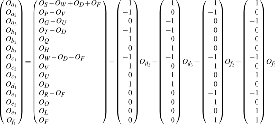
From the four contingency tables shown in Tables 2–4, it is easy to get the following linear equation system:

The rank of the above linear system is 14. We thus take 14 rows {4, 6, 10, 11, 12, 13, 14, 15, 16, 17, 18, 19, 20, 21}, which form a full rank matrix. The row reduced echelon form of this non-redundant linear system is

Thus, we have the following solution:

Clearly, only four variables {O_d2, O_d3, O_f2, O_f3} are free. Once the values of these free variables are known, the observed frequencies of remaining events in the two-locus contingency table are also known.

Proof of Theorem 5.1

Proof. —

It suffices to show that

This is the same as to show that

This is clearly true, hence completes the proof.

REFERENCES

- Balding DJ. A tutorial on statistical methods for population association studies. Nat. Rev. Genet. 2006;7:781–791. doi: 10.1038/nrg1916. [DOI] [PubMed] [Google Scholar]
- Carlborg O, et al. The use of a genetic algorithm for simultaneous mapping of multiple interacting quantitative trait loci. Genetics. 2000;155:2003–2010. doi: 10.1093/genetics/155.4.2003. [DOI] [PMC free article] [PubMed] [Google Scholar]
- Churchill GA, Doerge RW. Empirical threshold values for quantitative trait mapping. Genetics. 1994;138:963–971. doi: 10.1093/genetics/138.3.963. [DOI] [PMC free article] [PubMed] [Google Scholar]
- Cormen TH, et al. Introduction to Algorithms. MIT Press and McGraw-Hill; 2001. [Google Scholar]
- Dudoit S, Laan MJ. Multiple Testing Procedures with Applications to Genomics. Springer; 2008. [Google Scholar]
- Eisner J. State-of-the-art algorithms for minimum spanning trees: a tutorial discussion. Manuscript,University of Pennsylvania; 1997. [Google Scholar]
- Evans DM, et al. Two-stage two-locus models in genome-wide association. PLoS Genet. 2006;2:e157. doi: 10.1371/journal.pgen.0020157. [DOI] [PMC free article] [PubMed] [Google Scholar]
- Graham RL, Hell P. On the history of the minimum spanning tree problem. Ann. History Comput. 1985;7:43–57. [Google Scholar]
- Hirschhorn JN, Daly MJ. Genome-wide association studies for common diseases and complex traits. Nat. Rev. Genet. 2005;6:95–108. doi: 10.1038/nrg1521. [DOI] [PubMed] [Google Scholar]
- Hoh J, Ott J. Mathematical multi-locus approaches to localizing complex human trait genes. Nat. Rev. Genet. 2003;4:701–709. doi: 10.1038/nrg1155. [DOI] [PubMed] [Google Scholar]
- Hoh J, et al. Selecting snps in two-stage analysis of disease association data: a model-free approach. Ann. Hum. Genet. 2000;64:413–417. doi: 10.1046/j.1469-1809.2000.6450413.x. [DOI] [PubMed] [Google Scholar]
- Lewontin RC, Kojima K. The evolutionary dynamics of complex polymorphisms. Evolution. 1960;14:458–472. [Google Scholar]
- Miller RG. Simultaneous Statistical Inference. New York: Springer; 1981. [Google Scholar]
- Musani SK, et al. Detection of gene x gene interactions in genome-wide association studies of human population data. Hum. Hered. 2007;63:67–84. doi: 10.1159/000099179. [DOI] [PubMed] [Google Scholar]
- Nelson MR, et al. A combinatorial partitioning method to identify multilocus genotypic partitions that predict quantitative trait variation. Genome Res. 2001;11:458–470. doi: 10.1101/gr.172901. [DOI] [PMC free article] [PubMed] [Google Scholar]
- Ritchie MD, et al. Multifactor-dimensionality reduction reveals high-order interactions among estrogen-metabolism genes in sporadic breast cancer. Am. J. Hum. Genet. 2001;69:138–147. doi: 10.1086/321276. [DOI] [PMC free article] [PubMed] [Google Scholar]
- Roberts A, et al. Inferring missing genotypes in large snp panels using fast nearest-neighbor searches over sliding windows. Proceeding of ISMB. 2007 doi: 10.1093/bioinformatics/btm220. [DOI] [PubMed] [Google Scholar]
- Saxena R, et al. Genome-wide association analysis identifies loci for type 2 diabetes and triglyceride levels. Science. 2007;316:1331–1336. doi: 10.1126/science.1142358. [DOI] [PubMed] [Google Scholar]
- Scuteri A, et al. Genome-wide association scan shows genetic variants in the fto gene are associated with obesity-related traits. PLoS Genet. 2007;3:1200–1210. doi: 10.1371/journal.pgen.0030115. [DOI] [PMC free article] [PubMed] [Google Scholar]
- The Wellcome Trust Case Control Consortium. Genome-wide association study of 14,000 cases of seven common diseases and 3,000 shared controls. Nature. 2007;447:661–678. doi: 10.1038/nature05911. [DOI] [PMC free article] [PubMed] [Google Scholar]
- Wade CM, Daly MJ. Genetic variation in laboratory mice. Nat. Genet. 2005;37:1175–1180. doi: 10.1038/ng1666. [DOI] [PubMed] [Google Scholar]
- Weedon M, et al. A common variant of hmga2 is associated with adult and childhood height in the general population. Nat. Genet. 2007;39:1245–1250. doi: 10.1038/ng2121. [DOI] [PMC free article] [PubMed] [Google Scholar]
- Westfall PH, Young SS. Resampling-based Multiple Testing. New York: Wiley; 1993. [Google Scholar]
- Wright FA, et al. Simulating association studies: a data-based resampling method for candidate regions or whole genome scans. Bioinformatics. 2007;23:2581–2588. doi: 10.1093/bioinformatics/btm386. [DOI] [PubMed] [Google Scholar]
- Yang C, et al. SNPHarvester: a filtering-based approach for detecting epistatic interactions in genomewide association studies. Bioinformatics. 2009;25:504–511. doi: 10.1093/bioinformatics/btn652. [DOI] [PubMed] [Google Scholar]
- Zhang X, et al. FastANOVA: an efficient algorithm for genome-wide association study. Proceeding of KDD. 2008 [PMC free article] [PubMed] [Google Scholar]
- Zhang X, et al. COE: a general approach for efficient genome-wide two-locus epistatic test in disease association study. Proceeding of RECOMB. 2009a doi: 10.1089/cmb.2009.0155. [DOI] [PubMed] [Google Scholar]
- Zhang X, et al. FastChi: an efficient algorithm for analyzing gene-gene interactions. Proceeding of PSB. 2009b [PMC free article] [PubMed] [Google Scholar]