On quantifying the magnitude of confounding

Abstract

When estimating the association between an exposure and outcome, a simple approach to quantifying the amount of confounding by a factor, Z, is to compare estimates of the exposure–outcome association with and without adjustment for Z. This approach is widely believed to be problematic due to the nonlinearity of some exposure-effect measures. When the expected value of the outcome is modeled as a nonlinear function of the exposure, the adjusted and unadjusted exposure effects can differ even in the absence of confounding (Greenland , Robins, and Pearl, 1999); we call this the nonlinearity effect. In this paper, we propose a corrected measure of confounding that does not include the nonlinearity effect. The performances of the simple and corrected estimates of confounding are assessed in simulations and illustrated using a study of risk factors for low birth–weight infants. We conclude that the simple estimate of confounding is adequate or even preferred in settings where the nonlinearity effect is very small. In settings with a sizable nonlinearity effect, the corrected estimate of confounding has improved performance.

1. INTRODUCTION

Confounding is a perpetual challenge in epidemiological research. Assessing the amount of confounding is important for determining whether or not a specific factor should be statistically adjusted in the analysis. In addition, reporting the amount of confounding by a particular factor can aid in interpreting unadjusted associations reported in other studies. As an example, consider the association between maternal uterine irritability and the incidence of low birth–weight infants. Smoking is a possible confounder, being a known risk factor for low-birth weight and also a potential contributor to uterine irritability. A simple approach to quantifying confounding by smoking would be to compare odds ratios relating uterine irritability and low-birth weight with and without adjustment for smoking, that is, conditional and marginal odds ratios (see e.g. Breslow and Day, 1980; Kleinbaum and others, 1982). We call this the simple approach to quantifying confounding. Many have cautioned against this approach, pointing out that conditional and marginal effect measures can differ absent confounding, and that confounding can occur even when conditional and marginal effect measures are equal (Miettinen and Cook, 1981; Greenland and Robins, 1986; Wickramaratne and Holford, 1987; Greenland , Robins, and Pearl, 1999; Greenland and Morgenstern, 2001. This situation can occur when the measure of exposure effect is nonlinear.

In this paper, we develop a statistical framework that distinguishes the magnitude of confounding from the size of the nonlinearity effect. We show that the simple measure of confounding combines the true confounding bias with the magnitude of the nonlinearity effect. We develop a corrected measure of confounding and associated methods for estimation and inference. Using simulations, we compare the performance of the simple and corrected estimates of confounding. We find that, in scenarios where the nonlinearity effect is very small, the simple estimate of confounding is adequate or even preferred. With a sizeable nonlinearity effect, the corrected estimate of confounding yields improved performance.

2. STATISTICAL FRAMEWORK

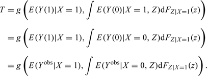
We define confounding bias using the potential outcomes framework of Neyman (1923) and Rubin (1974, 1978) as discussed by Greenland , Robins, and Pearl (1999), Greenland and Morgenstern (2001), and Maldonado and Greenland (2002). Let X denote the observed binary exposure and Y^obs the observed outcome. The methods are generalized to a continuous exposure in Section 1 of the supplementary material available at Biostatistics online. Denote by Y(1) and Y(0) the potential outcomes with and without exposure. That is, Y(0) is the outcome that would be observed if a subject was not exposed, and Y(1) is the outcome that would be observed if the subject was exposed. Our interest lies in estimating the causal effect of exposure on the outcome among a set of exposed subjects (X = 1). We compare the outcomes for the exposed subjects with their expected outcomes had they not been exposed using

(2.1)

where g is a measure of the exposure effect such as a log relative risk or log odds ratio. T is defined as the causal exposure effect among the exposed (Greenland , Robins, and Pearl, 1999; Greenland and Morgenstern, 2001; Hernan, 2004; Hernan and Robins, 2006). This is a sensible measure of exposure effect for harmful exposures. Section 3 of the supplementary material available at Biostatistics online extends the approach to other measures of causal exposure effect.

3. QUANTIFYING CONFOUNDING

The causal exposure effect defined in (2.1) is not directly observable. Specifically, E(Y(1)|X = 1) = E(Y^obs|X = 1) is observable but E(Y(0)|X = 1) is not. Suppose that we have data for a population of unexposed individuals to serve as a reference. Let

(3.1)

be the marginal exposure effect utilizing the reference population. Note that T_m depends only on observable quantities since E(Y(1)|X = 1) = E(Y^obs|X = 1) and E(Y(0)|X = 0) = E(Y^obs|X = 0). As in Greenland , Robins, and Pearl (1999), Greenland and Morgenstern (2001), and Maldonado and Greenland (2002), we define confounding as any difference between the causal exposure effect (T) and the marginal exposure effect (T_m). Confounding is then a consequence of factors other than exposure that differ between the unexposed and exposed groups.

Consider one or more covariates, Z, that explain the confounding or difference between exposed and unexposed groups. In other words, assume that the potential outcome Y(0) is independent of exposure given Z so that, within strata of Z, those exposed have the same distribution of Y(0) as those unexposed. Under this assumption E(Y(0)|X = 1,Z) = E(Y(0)|X = 0,Z), and the causal exposure effect T can be rewritten as

(3.2)

Note that all the quantities in (3.2) are now directly observable. In addition, expression (3.2) shows that the causal exposure effect is obtained by reweighting the unexposed observations with respect to the distribution of Z in the exposed population.

The magnitude of confounding bias can thus be written as

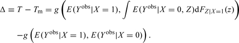(3.3)

Observe that (3.3) reduces to zero if the distribution of Z is the same in the exposed and unexposed populations. This occurs, for example, when the 2 populations are matched with respect to Z.

Given a random sample of exposed and unexposed individuals, we estimate the magnitude of confounding (Δ = T − T_m) in 2 different ways. We utilize estimators of the causal exposure effect (T) described by Hernan and Robins (2006) and Sato and Matsuyama (2003). With the first approach, the quantities in (3.3) are estimated directly:

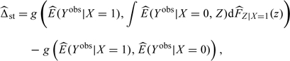(3.4)

where (Y^obs|X = 1), (Y^obs|X = 0), and Z | X = 1 are empirical estimates and (Y^obs|X = 0, Z) is obtained from a binary regression model. Following Hernan and Robins (2006) and Sato and Matsuyama (2003), we refer to this as the standardization estimator of Δ. Bootstrapping is used for inference.

For the second estimation approach, note that E(Y(0)|X = 1) is equivalent to

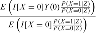which is an inverse probability weighted (IPW) mean with weights P(X = 1|Z)/P(X = 0|Z) (Hernan and Robins, 2006). Hence, T can be estimated by

(3.5)

where E(Y^obs|X = 1) is estimated empirically and P(X = 1|Z) is estimated by using a binary regression model such as logistic regression (Hernan and Robins, 2006; Hernan, 2004; Sato and Matsuyama, 2003). Subtracting from this the estimated marginal exposure effect () yields the IPW estimate of confounding bias,

(3.6)

We note that for discrete Z, the standardization and IPW estimates of Δ are the same (_st = _IPW) but they differ otherwise (Hernan and Robins, 2006). Bootstrapping is used for inference for its flexibility, although asymptotic variance expressions could also be used (Robins, 1998; Robins, 1999).

4. QUANTIFYING THE NONLINEARITY OF THE EXPOSURE EFFECT

The potential outcomes framework also provides a simple definition of the nonlinearity effect. Consider the causal effect of exposure, X, on the outcome, Y, conditional on the covariate, Z:

(4.1)

As indicated by the notation, to isolate the issue of confounding, we assume that Z is not an effect modifier, in other words that T_c is constant across the levels of Z. We say that a measure of association g incorporates a nonlinearity effect over Z if the conditional exposure effect (T_c) differs from the causal exposure effect (T). Observe that the nonlinearity effect is not due to confounding by Z; by definition neither T nor T_c are confounded by Z.

Neither the rate difference nor the log relative risk incorporate nonlinearity effects, but the log odds ratio does. Neuhaus and others (1991) considered nonlinearity effects in the context of marginal and random-effects logistic models for correlated binary data; in our setting Z behaves as the random effect. They show that for the log odds ratio, |T_c| ≥ |T|, and

(4.2)

for the logistic regression model:logoddsE(Y|X,Z) = β₀ + β_xX + β_zZ, where logoddsp_z = β₀ + β_zZ and q_z = 1 − p_z. In other words, the size of the nonlinearity effect depends on the effects of X and Z on Y and on the variance of Z.

The simple approach to quantifying confounding contrasts conditional and marginal effect measures (T_c − T_m). In the epidemiologic literature, a measure for which T_c≠T_m is not “strictly collapsible” (Greenland , Robins, and Pearl, 1999; Greenland and Morgenstern, 2001). The difference T_c − T_m includes both bias due to confounding and the nonlinearity effect. To see this, we write

(4.3)

The first component (T − T_m = Δ) is confounding bias. The second component (T_c − T = Δ_nl) is the size of the nonlinearity effect. As discussed above, the second component reduces to zero when g is the risk difference or log relative risk but not when g is the log odds ratio. Therefore, when the log odds ratio is the parameter of interest, T_c − T_m is generally an inaccurate measure of confounding because it includes the nonlinearity effect. In Section 5, we compare the properties of the simple measure of confounding (T_c − T_m) and the corrected measure of confounding (T − T_m) when the parameter of interest is a log odds ratio.

5. SIMULATION STUDIES

We consider the logistic model for a binary outcome and a binary exposure. The continuous exposure case is discussed in Section 1 of the supplementary material. Three estimates of confounding bias are compared in terms of bias and variability: the simple estimate,

(5.1)

which includes the nonlinearity effect, and 2 estimates of the corrected measure of confounding that do not include the nonlinearity effect, the standardization estimate (3.4) and the IPW estimate (3.6).

We simulate 5000 data sets with 1000 exposed and 1000 unexposed subjects under the following model:

(5.2)

with β₀ = − 3, α₀ = 0, and a modest conditional exposure effect, e^β₁ = 2.0. The parameters α₁ and β₂ are varied to explore different scenarios. We consider the causal log odds ratio, T, the confounding bias Δ = T − T_m, and the size of the nonlinearity effect, Δ_nl = T_c − T.

Each scenario is displayed graphically using a plot of E(Y|X,Z) versus Z, for each value of X (see Table 1). These plots visually display the size of the exposure effect, the amount of confounding, and the size of the nonlinearity effect. The length of the lines is governed by the interquartile range of Z|X, and the dot on each line is at the marginal mean E(Z|X). The vertical separation between the lines for X = 0 and X = 1 displays the size of the conditional exposure effect. The horizontal separation between the lines is due to differences in the Z-distribution between exposed and unexposed populations, and thus represents the amount of confounding. Finally, the curvature of the lines measures the degree of nonlinearity of E(Y|X,Z) as function of Z and therefore captures the nonlinearity effect.

Table 1.

5000 simulations under model (5.2) to evaluate the performance of the 3 estimates of confounding bias for a binary exposure. In each scenario, E(Y|X, Z) is plotted against Z for each value of X. In all scenarios, e^β₁ = 2.0. The mean Neuhaus and others (1991) estimate of the nonlinearity effect is also shown

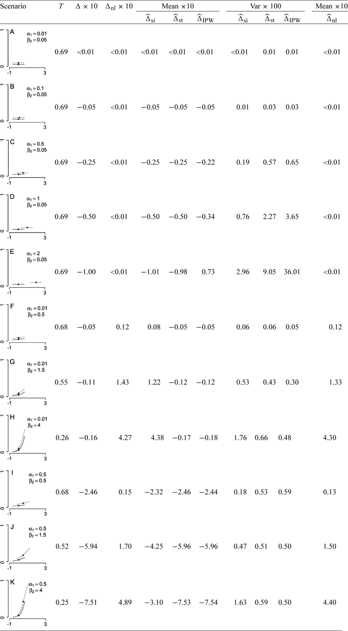The performances of the estimators of confounding bias are displayed in Table 1. When there is negligible confounding and nonlinearity effect (both < 1% of the size of the exposure effect; Scenarios A and B), the standardization and IPW estimators tend to be less biased but more variable than the simple estimator. As the amount of confounding bias increases (holding the nonlinearity effect under 1% of the size of the exposure effect; Scenarios C, D, and E), the simple and corrected estimates are all relatively unbiased, but the corrected estimates are substantially more variable. Note that the IPW estimator, in particular, performs poorly when the Z–X association is strong (Scenarios D and E), as P(X = 1|X) is close to 0 or 1 and the weights are extreme. When there is a large nonlinearity effect ( > 25% of the size of the exposure effect) but negligible confounding bias ( < 7% of the size of the exposure effect; Scenarios G and H), the simple estimator is substantially biased, and the corrected estimators are relatively unbiased and less variable. Finally when there is large confounding bias (> 30% of the size of the exposure effect; Scenarios I, J, and K), adding a nonlinearity effect makes the simple estimator biased; the corrected estimators are relatively unbiased but tend to be more variable.

The approximation of Neuhaus and others (1991) given in (4.2) is also used to estimate the nonlinearity effect in each scenario (Table 1). This approximation produces a reasonably unbiased estimate of the nonlinearity effect and can be used as a simple diagnostic to determine whether the nonlinearity effect is large enough to merit using a bias-corrected estimate of confounding.

We conclude that in scenarios with very small nonlinearity effects, the simple estimate of confounding bias, obtained by contrasting coefficients for the risk factor of interest from regression models with and without the confounders, is appropriate. Correcting for the small amount of bias comes at too high a cost in terms of extra variability. On the other hand, in circumstances where the nonlinearity effect is sizeable, the corrected estimates of confounding are less biased. But the reduction in bias may be associated with a confounding estimate with increased variability. By varying the size of the conditional exposure effect we find similar conclusions.

6. DATA ANALYSIS EXAMPLE

In this section, we use the data from a 1986 cohort study conducted at the Baystate Medical Center, Springfield Massachusetts (Hosmer and Lemeshow, 2000) to illustrate the various approaches to quantifying confounding. The study was designed to identify risk factors associated with giving birth to a low birth–weight baby (weighing less than 2500 grams). Data were collected on 189 pregnant women, 59 of whom had low birth–weight infants. We study the effect of uterine irritability (yes/no) on low-birth weight. Smoking status during pregnancy (yes/no) is a possible confounder. Smoking is well known to increase the risk of low-birth weight and may also be a contributor to uterine irritability. There is no significant evidence that smoking modifies the effect of uterine irritability on low-birth weight (p = 0.57, Wald test; see Table 2).

Table 2.

Low birth–weight study: uterine irritability, smoking, and low birth–weight status

Maternal uterine irritability	Low birth–weight infant
	No	Yes
Nonsmoking mother
No	78	22
Yes	8	7
Smoking mother
No	38	23
Yes	6	7

We estimate confounding by smoking using the standardization estimator (3.4); the IPW estimator is identical because the confounder is discrete. The components of (3.4) are estimated empirically, and confidence intervals are based on quantiles of distributions of estimates across 1000 bootstrap samples.

The estimates of confounding and nonlinearity effect are shown in Table 3. With the standardization estimator, we calculate that the confounding due to smoking in the marginal log odds ratio is = − 0.07 (95% CI: − 0.27 to 0.09). Since e^0.07 = 1.07, this implies that confounding by smoking magnifies the marginal odds ratio by 7% (95% CI: 9% attenuation to 31% magnification). The estimated marginal odds ratio confounded by smoking is 2.58 (95% CI: 1.07–5.89), while the estimated marginal odds ratio unconfounded by smoking is 2.41 (95% CI: 1.01–5.50).

Table 3.

Estimates of confounding bias (Δ) and nonlinearity effect (Δ_nl) in the low birth–weight study. Smoking confounds the log odds ratio relating uterine irritability and low birth–weight. Simple (5.1) and standardization (3.4) estimates are shown along with 95% CI based on bootstrap resampling. IPW estimates are identical to the standardization estimates

	(CI)	nl (CI)
Simple	− 0.03 (− 0.21, 0.14)	—
Standardization	− 0.07 (− 0.27, 0.09)	0.03 (− 0.02, 0.12)

Compare this to the simple estimate of confounding, defined as the difference in log odds ratios from logistic regression models with and without smoking status. We estimate that confounding by smoking magnifies the odds ratio by 3% (95% CI: 13% attenuation to 24% magnification). This is a slight underestimate of the magnitude of confounding; it includes both bias due to confounding and the effect of nonlinearity of the odds ratio. The nonlinearity effect is relatively small; we estimate that the conditional odds ratio is 3% larger than the marginal odds ratio, absent confounding by smoking (95% CI: 2% smaller to 13% larger).

When estimating confounding using the standardization estimator versus the simple estimator, we see that there is a slight increase in variability. This is consistent with what we saw in the simulations. In Scenarios F and I, where the nonlinearity effects are of comparable size, the corrected estimates of confounding are less biased and have similar or slightly more variability than the simple confounding estimate.

7. DISCUSSION

Much of the epidemiologic literature places an emphasis on the distinction between confounding bias and nonlinearity in the measure of exposure effect (Miettinen and Cook, 1981; Greenland and Robins, 1986; Wickramaratne and Holford, 1987; Greenland , Robins, and Pearl, 1999; Greenland and Morgenstern, 2001). The simple approach to quantifying confounding, by contrasting the conditional and marginal effect estimates, is not advocated. Statistical methods have been developed to compare conditional and marginal effect estimates (Hausman, 1978; Whittemore, 1978; Greenland and Maldonado, 1994; Ducharme and Lepage, 1986; Greenland and Mickey, 1988; Hoffmann and others, 2008), but as we have seen this contrast includes both bias due to confounding and the magnitude of the nonlinearity effect. In this paper, we propose a corrected approach that separates confounding bias from nonlinearity effect. We develop estimates of both the true confounding bias and the magnitude of the nonlinearity effect.

Under a linear or log-linear model, there is no nonlinearity effect and therefore the simple estimate of confounding defined in (5.1) is unbiased. Under a logistic model, the simple measure can be biased. Using simulations, we explored the performance of the corrected estimates of confounding. Section 1 of the supplementary material available at Biostatistics online extends these simulations to the continuous exposure case. We found that when there is a sizeable nonlinearity effect, the corrected estimate of confounding is preferred. The classic examples of nonlinearity effects in the literature are such scenarios. For instance, the example shown in Table 1 of Greenland , Robins, and Pearl (1999) has no confounding (Δ = 0) and a very large nonlinearity effect (Δ_nl = 0.17; 21% of the size of the exposure effect); here the corrected estimate of confounding is warranted. However, when the nonlinearity effect is small, the simple estimate of confounding is appropriate since correcting for the small linearity effect incurs a cost of extra variability in the estimate of confounding. The estimate of the nonlinearity effect based on the approximation of Neuhaus and others (1991) can be used as a simple diagnostic to determine whether separating confounding and the nonlinearity effect is warranted.

The approach presented here can be generalized. First, it can be used to quantify confounding due to one factor over and above known confounders. We extend the methods to this setting in the Section 2 of the supplementary material available at Biostatistics online. Second, we have used the causal exposure effect among exposed individuals as the basis for the approach to quantifying confounding. The methods can easily be extended to settings where the exposure effect among the total population is of interest, as shown in Section 3 of the supplementary material available at Biostatistics online.

Care should be taken to determine whether it is appropriate to condition on a variable in any given data analysis. Causal diagrams are useful tools for identifying confounders for conditioning (Pearl, 1995; Pearl, 2000; Greenland , Pearl, and Robins, 1999). They provide a general framework for identifying the variables that should be conditioned on to avoid bias due to confounding or selection bias. Causal diagrams can also be used to identify variables that should not be conditioned on. For example, a more detailed treatment is required of a variable that is an intermediate step between exposure and disease (Robins, 1989; Robins and Greenland, 1992). Conditioning on “collider variables,” which are affected by both exposure and outcome, can actually create bias (Greenland, 2003). However, causal diagrams do not provide information about the magnitude of bias due to lack of conditioning. This is the focus of our work: given a confounder, we propose an approach to quantify the bias resulting from it.

Our approach assumes that the confounders have been measured. There is, however, a large literature on methods for quantifying confounding due to unmeasured factors. Sensitivity analyses make assumptions about the behavior of the unmeasured confounders, calculate the associated bias, and then vary the assumed values over a range to assess the potential magnitude of confounding (see e.g. Cornfield and others, 1959; Gail and others, 1988; Rosenbaum 2002). Alternatively, a probabilistic approach can be used wherein a distribution is assumed for the unknown parameters and incorporated into the measure of confounding bias (see e.g. Lash and Silliman, 2000, Greenland, 2001, Greenland, 2003, Greenland, 2005, Phillips, 2003).

We have assumed throughout that there is no effect modification. When Z modifies the exposure effect, primary interest lies in the conditional exposure effect T_c(Z) as it varies with Z. However, an overall exposure effect may also be obtained by averaging the conditional effects. For nonlinear exposure–effect measures, the average conditional exposure effect T^* = ∫T_c(Z)dG(Z), where G is an arbitrary measure, will differ from the marginal exposure effect T_m. This is also called noncollapsibility of the exposure effect (Greenland , Robins, and Pearl, 1999; Greenland and Morgenstern, 2001). Our methods can be used to show that T^* − T_m = T − T_m + T^* − T and to distinguish confounding bias (T − T_m) from the nonlinearity effect (T^* − T).

SUPPLEMENTARY MATERIAL

Supplementary material is available at http://biostatistics.oxfordjournals.org.

FUNDING

National Institute of Environmental Health Sciences (Award Numbers R01ES012054 and R83622 and EPA RD83241701).

References

- Breslow NE, Day NE. Statistical Methods in Cancer Research Volume 1: Analysis of Case-Control Data. Geneva, Switzerland: World Health Organization; 1980. [PubMed] [Google Scholar]
- Cornfield J, Haenszel W, Hammond EC, Lilienfeld AM, Shimkin MB, Wynder EL. Smoking and lung cancer: recent evidence and a discussion of some questions. Journal of the National Cancer Institute. 1959;22:173–203. [PubMed] [Google Scholar]
- Ducharme GR, Lepage Y. Testing collapsibility in contingency tables. Journal of the Royal Statistical Society, Series B. 1986;48:197–205. [Google Scholar]
- Gail MH, Wacholder S, Lubin JH. Indirect corrections for confounding under multiplicative and additive models. American journal of industrial medicine. 1988;13:119–130. doi: 10.1002/ajim.4700130108. [DOI] [PubMed] [Google Scholar]
- Greenland S. Sensitivity analysis, Monte-Carlo risk analysis, and Bayesian uncertainty assessment. Risk Analysis. 2001;21:579–583. doi: 10.1111/0272-4332.214136. [DOI] [PubMed] [Google Scholar]
- Greenland S. The impact of prior distributions for uncontrolled confounding and response bias: a case study of the relation of wire codes and magnetic fields to childhood leukemia. Journal of the American Statistical Association. 2003;98:47–54. [Google Scholar]
- Greenland S. Multiple-bias modeling for analysis of observational data (with discussion) Journal of the Royal Statistical Society, Series A. 2005;168:267–308. [Google Scholar]
- Greenland S, Maldonado G. Inference on collapsibility in generalized linear models. Biometrical Journal. 1994;36:771–782. [Google Scholar]
- Greenland S, Mickey RM. Closed form and dually consistent methods for inference on strict collapsibility in 2 x 2 x K and 2 x J x K tables. Applied Statistics. 1988;37:335–343. [Google Scholar]
- Greenland S, Morgenstern H. Confounding in health research. Annual Review of Public Health. 2001;22:189–212. doi: 10.1146/annurev.publhealth.22.1.189. [DOI] [PubMed] [Google Scholar]
- Greenland S, Pearl J, Robins JM. Causal diagrams for epidemiologic research. Epidemiology. 1999;10:37–48. [PubMed] [Google Scholar]
- Greenland S, Robins JM. Identifiability, exchangeability, and epidemiological confounding. International Journal of Epidemiology. 1986;15:413–418. doi: 10.1093/ije/15.3.413. [DOI] [PubMed] [Google Scholar]
- Greenland S, Robins JM, Pearl J. Confounding and collapsibility in causal inference. Statistical Science. 1999;14:29–46. [Google Scholar]
- Hausman JA. Specification tests in econometrics. Econometrica. 1978;46:1251–1271. [Google Scholar]
- Hernan MA. A definition of causal effect for epidemiological research. Journal of Epidemiology and Community Health. 2004;58:265–271. doi: 10.1136/jech.2002.006361. [DOI] [PMC free article] [PubMed] [Google Scholar]
- Hernan MA, Robins JM. Estimating causal effects from epidemiological data. Journal of Epidemiology and Community Health. 2006;60:578–586. doi: 10.1136/jech.2004.029496. [DOI] [PMC free article] [PubMed] [Google Scholar]
- Hoffmann K, Pischon T, Schulz M, Schulze MB, Ray J, Boeing H. A statistical test for the equality of differently adjusted incidence rate ratios. American Journal of Epidemiology. 2008;167:512–522. doi: 10.1093/aje/kwm357. [DOI] [PubMed] [Google Scholar]
- Hosmer DW, Lemeshow S. Applied Logistic Regression. 2nd edition. New York: John Wiley and Sons; 2000. [Google Scholar]
- Kleinbaum DG, Kupper LL, Morgenstern H. Epidemiologic Research. Belmont, CA: Lifetime Learning Publications; 1982. [Google Scholar]
- Lash TL, Silliman RA. A sensitivity analysis to separate bias due to confounding from bias due to predicting misclassification by a variable that does both. Epidemiology. 2000;11:544–549. doi: 10.1097/00001648-200009000-00010. [DOI] [PubMed] [Google Scholar]
- Maldonado G, Greenland S. Estimating causal effects. International Journal of Epidemiology. 2002;31:422–429. [PubMed] [Google Scholar]
- Miettinen OS, Cook EF. Confounding: essence and detection. American Journal of Epidemiology. 1981;114:593–603. doi: 10.1093/oxfordjournals.aje.a113225. [DOI] [PubMed] [Google Scholar]
- Neuhaus JM, Kalbfleisch JD, Hauck WW. A comparison of cluster-specific and population-averaged approaches for analyzing correlated binary data. International Statistical Review. 1991;59:25–35. [Google Scholar]
- Neyman J. On the application of probability theory to agricultural experiments: essay on principles, section 9. Statistical Science. 1923;5:465–480. (Translated) [Google Scholar]
- Pearl J. Causal diagrams for empirical research. Biometrika. 1995;82:669–710. [Google Scholar]
- Pearl J. Causality. New York: Cambridge University Press; 2000. [Google Scholar]
- Phillips CV. Quantifying and reporting uncertainty from systematic errors. Epidemiology. 2003;14:459–466. doi: 10.1097/01.ede.0000072106.65262.ae. [DOI] [PubMed] [Google Scholar]
- Robins JM. The control of confounding by intermediate variables. Statistics in Medicine. 1989;8:679–701. doi: 10.1002/sim.4780080608. [DOI] [PubMed] [Google Scholar]
- Robins JM. Marginal structural models. 1997 Proceedings of the Section on Bayesian Statistical Science. Alexandria, VA: American Statistical Association; 1998. pp. 1–10. [Google Scholar]
- Robins JM. Marginal structural models versus structural nested models as tools for causal inference. In: Halloran E, Berry D, editors. Statistical Models in Epidemiology: The Environment and Clinical Trials. New York: Springer; 1999. pp. 95–134. [Google Scholar]
- Robins JM, Greenland S. Identifiability and exchangeability for direct and indirect effects. Epidemiology. 1992;3:143–155. doi: 10.1097/00001648-199203000-00013. [DOI] [PubMed] [Google Scholar]
- Rosenbaum PR. Observational Studies. 2nd edition. New York: Springer; 2002. [Google Scholar]
- Rubin DB. Estimating causal effects of treatments in randomized and nonrandomized studies. Journal of Educational Psychology. 1974;66:688–701. [Google Scholar]
- Rubin DB. Bayesian inference for causal effects: the role of randomization. Annals of Statistics. 1978;6:34–58. [Google Scholar]
- Sato T, Matsuyama Y. Marginal structural models as a tool for standardization. Epidemiology. 2003;14:680–686. doi: 10.1097/01.EDE.0000081989.82616.7d. [DOI] [PubMed] [Google Scholar]
- Wickramaratne PJ, Holford TR. Confounding in epidemiologic studies: the adequacy of the control group as a measure of confounding. Biometrics. 1987;43:751–765. [PubMed] [Google Scholar]
- Whittemore AS. Collapsibility of multidimensional contingency tables. Journal of the Royal Statistical Society, Series B. 1978;40:328–340. [Google Scholar]
Associated Data
This section collects any data citations, data availability statements, or supplementary materials included in this article.