Searching for Autocoherence in the Cortical Network with a Time-Frequency Analysis of the Local Field Potential

Abstract

Gamma-band peaks in the power spectrum of local field potentials (LFP) are found in multiple brain regions. It has been theorized that gamma oscillations may serve as a ‘clock’ signal for the purposes of precise temporal encoding of information and ‘binding’ of stimulus features across regions of the brain. Neurons in model networks may exhibit periodic spike firing or synchronized membrane potentials that give rise to a gamma-band oscillation that could operate as a ‘clock’. The phase of the oscillation in such models is conserved over the length of the stimulus. We define these types of oscillations to be ‘autocoherent’. We investigated the hypothesis that autocoherent oscillations are the basis of the experimentally observed gamma-band peaks: the autocoherent oscillator (ACO) hypothesis. To test the ACO hypothesis, we developed a new technique to analyze the autocoherence of a time-varying signal. This analysis used the continuous Gabor transform to examine the time evolution of the phase of each frequency component in the power spectrum. Using this analysis method, we formulated a statistical test to compare the ACO hypothesis with measurements of the LFP in macaque primary visual cortex, V1. The experimental data were not consistent with the ACO hypothesis. Gamma-band activity recorded in V1 did not have the properties of a ‘clock’ signal during visual stimulation. We propose instead that the source of the gamma-band spectral peak is the resonant V1 network driven by random inputs.

Introduction

Gamma-band (25 to 90 Hz) oscillations occur in many parts of the brain. We are seeking to understand the underlying neural mechanisms that generate gamma-band spectral peaks in the cerebral cortex by studying gamma activity in the local field potential (LFP) in the primary visual cortex, V1. The LFP is commonly interpreted as a measure of local network activity (Kruse and Eckhorn, 1996; Logothetis et al., 2001; Buzsaki, 2006). Previous experimental studies of V1 have reported a peak in the gamma-band of the LFP power spectrum when the visual cortex was visually driven (Gray and Singer, 1989; Gray et al., 1989; Frien et al., 2000; Logothetis et al., 2001; Siegel and Konig, 2003; Henrie and Shapley, 2005).

The presence of gamma-band activity in many LFP measurements under stimulation led to the idea that gamma-band oscillations serve as a ‘clock’ signal for the purpose of temporally encoding information (Hopfield, 1995; Buzsaki and Chrobak, 1995; Jefferys et al., 1996; Buzsaki and Draguhn, 2004; Buzsaki, 2006; Bartos et al., 2007; Fries et al., 2007; Hopfield, 2004). The ‘clock’ theory of gamma combined with the pervasiveness of gamma oscillations have given rise to the theory that the brain uses gamma oscillations to synchronize different regions of the brain for the purpose of ‘binding’ information about a stimulus (Gray and Singer, 1989; Singer and Gray, 1995).

Many studies of neuronal network models have sought to explain the mechanisms underlying gamma-band activity through either quasi-periodic spike firing, synchronized oscillatory spiking, or rhythmic subthreshold membrane potential oscillations (see Results, Oscillator models of the LFP). We define an oscillation that can be modeled as a sinusoid with a fixed phase that does not vary with time to be ‘autocoherent’. A shared feature of many network models of gamma oscillations is that they generate an autocoherent network oscillation as an equilibrium state of the network. Autocoherence is an essential feature of such models because they were designed to yield gamma oscillations that could be used as a clock signal. We refer to the hypothesis that autocoherent oscillations underlie experimentally observed gamma-band spectral peaks as the autocoherent oscillator (ACO) hypothesis.

The aim of this study was to test the ACO hypothesis. We analyzed LFP measurements recorded from V1 cortex. Visual stimulation evoked a noisy LFP response in V1, with a peak of spectral power in the gamma-band. We developed a new method of signal processing to search for either constant amplitude or amplitude-modulated autocoherent signals embedded in the LFP. Our technique uses the continuous Gabor transform (CGT; Mallat, 1999; see Methods) to investigate LFP phase portraits at each temporal frequency. Using the CGT, we formulated a statistical test to compare the ACO hypothesis with LFP data from V1 cortex. In brief, we performed a rigorous search for autocoherent oscillations in visually-driven V1 activity and did not find them; the data did not support the ACO hypothesis. This result rules out a class of models that predicts that gamma activity is generated by a deterministic mechanism that produces a constant-phase clock signal. Our interpretation is that the source of the gamma-band peak is of a stochastic nature, a hypothesis considered in the Discussion.

Materials and Methods

Experimental Procedure

Surgery and preparation.

Acute experiments were performed on adult Old World monkeys (Macaca fascicularis). All surgical and experimental procedures were performed in accordance with the guidelines of the U.S. Department of Agriculture and have been approved by the University Animal Welfare Committee at New York University. Animals were tranquilized with acepromazine (50 μg/kg, i.m.) and anesthetized initially with ketamine (30 mg/kg, i.m.) and then with isofluorane (1.5% to 3.5% in air). After cannulation and tracheotomy, the animal was placed in a stereotaxic frame and was maintained on opioid anesthetic (sufentanil citrate, 6 to 12 μg kg⁻¹ h⁻¹, i.v.) for craniotomy. A craniotomy (about 5 mm in diameter) was made in one hemisphere posterior to the lunate sulcus (15 mm anterior to the occipital ridge, 10 to 20 mm lateral from the midline). A small opening in the dura (3 × 3 mm²) was made to provide access for multiple electrodes. After surgery, the animal was anesthetized and paralyzed with a continuous infusion of sufentanil citrate (6 to 12 μg kg⁻¹ h⁻¹, i.v.) and vecuronium bromide (0.1 mg kg⁻¹ h⁻¹, i.v.). Vital signs, including heart rate, electroencephalogram, blood pressure, oxygen level in blood, and urine-specific gravity were closely monitored throughout the experiment. Expired carbon dioxide was maintained close to 5%, and body temperature was kept at a constant 37°C. A broad-spectrum antibiotic (Bicillin, 50,000 iu/kg, i.m.) and anti-inflammatory steroid (dexamethasone, 0.5 mg/kg, i.m.) were given on the first day and every other day during the experiment. The eyes were treated with 1% atropine sulfate solution to dilate the pupils and with a topical antibiotic (gentamicin sulfate, 3%) before being covered with gas-permeable contact lenses. Foveae were mapped onto a tangent screen using a reversing ophthalmoscope. Proper refraction was achieved by placing corrective lenses in front of the eyes on custom-designed lens holders.

Electrophysiological recordings and data acquisition.

The Thomas 7-electrode system was used to record simultaneously from multiple cortical cells in V1. The seven electrodes were arranged in a straight line with each electrode separated from its neighbor by 300 μm. The electrodes had impedance values in the range 0.7 to 4 Megohms. Electrical signals from the seven electrodes were amplified, digitized, and filtered (0.3 to 10 kHz) with RA16SD preamplifiers in a Tucker-Davis System 3. The Tucker-Davis system was interfaced to a Dell PC computer. Visual stimuli were generated with the custom OPEQ program (written by Dr. J.A. Henrie), running in Linux on a Dell PC with an off-the-shelf graphics card. Data collection was synchronized with the screen refresh to a precision of better than 0.01 ms. Stimuli were displayed on an IIyama HM 204DTA flat Color Graphic Display (size, 40.38 × 30.22 cm²; pixels, 2048 × 1536; frame rate, 100 Hz; mean luminance, 53 cd/m²). The screen viewing distance was 115 cm.

Visual stimulation.

Once all seven electrodes were placed in V1 cortex, an experiment was run with drifting sinusoidal gratings (at high contrast [0.8], spatial frequency 2 cycle/deg, temporal frequency 4 Hz) that covered the visual fields of all the recording sites. The stimulus was drifted in 18 different directions between 0 and 360°, in 20° steps. The stimulus in each condition was presented for 2 or 4 s, repeated between 25 and 50 times depending on the experiment.

R-spectrum and spectral shape index

The R-spectrum, as used here, is defined to be the visual stimulated power spectrum divided frequency by frequency by the spontaneous power spectrum,

The R-spectrum is useful for expressing the stimulated power spectrum in normalized dimensionless units that can be compared across experiments. At frequencies where R > 1, the stimulated spectrum has elevated power in comparison to the spontaneous activity.

The spectral shape index (SSI) is a measure of how large a peak in the R-spectrum is in relation to its neighboring frequencies and is defined as (cf. Henrie and Shapley, 2005),

where R is the R-spectrum of Equation 1. The SSI is also dimensionless. When SSI > 1, a peak seen in the gamma-band R-spectrum sits above the average LFP power and forms a power spectral ‘bump’ about the maximum R-spectrum value.

Continuous Gabor transform

The continuous Gabor transform (CGT) is a short-time or windowed Fourier transform (also called a complex spectrogram) that retains the time dependence of the spectrum that is lost in the Fourier transform (Mallat, 1999). The continuous transform differs from the discrete version in that the signal is oversampled in time and frequency so that neighboring points are not independent. The Gabor filter ψ(t) used here is a one-dimensional plane wave with frequency ω₀ (in Hz) windowed with a Gaussian g(t) centered at t₀,

The CGT of a signal f (t) is found by convolving the Gabor function with f (t) and results in a complex time series R(t₀)e^iϕ(t0) that represents the amplitude and phase of the signal at the frequency of the Gabor filter,

In time-frequency analyses the uncertainty principle limits the resolution that can be resolved in the temporal and spectral domains. This limitation is expressed by the parameter σ in Equation 3. A balance between the time and frequency resolutions must be found that captures the characteristics of interest for the time series studied. If the characteristic width of the Gabor filter is considered to be two e-folding lengths (the distance at which the Gaussian envelope is e⁻² less than its peak value), the uncertainty condition for the CGT is

where δ_t is the characteristic time scale and δ_ω is the characteristic frequency scale. Here δ_t corresponds to the time scale of the LFP bursts (∼100 ms) which gives a frequency resolution of 6.4 Hz using Equation 5.

Phase portraits and phase rotation

The CGT, described in Equation 4, generates complex values that represent the amplitude and phase of the signal at the center frequency of the Gabor filter at each time step. The time dependence of the data is maintained by the CGT, as opposed to the Fourier transform, which is why this type of analysis is called a time-frequency analysis. Using the amplitude and phase at each frequency as functions of time, we can plot a phase portrait (in polar coordinates) for each frequency component that tracks the time evolution of the oscillation. In computing the CGT, the phase at each time step is computed with respect to the time at the center of the Gabor filter rather than with respect to the beginning of the record. To determine whether a frequency component is autocoherent, one must compare the phases at different time steps; the phases must be rotated to a common reference time. This rotation is performed by finding the phase shift of each time point relative to a reference point (here the first time point in the record) by computing the number of cycles that a sine wave at frequency ω oscillates during the time Δt that separates the time point from the reference point. The rotated phase ϕ_R of the time point is the measured local phase minus the phase shift Δϕ

where T = 1/ω is the period of the oscillation.

As an example, consider the phase portrait of an autocoherent (constant phase) sine wave. It has a trajectory that forms a circle as the CGT tracks the propagation of the local phase of the sine wave through time. To reveal that these data points are generated by a constant-phase sine wave, a phase shift, Δϕ, that represents the propagation of the sine wave is subtracted from each local phase point, ϕ(t,ω). This corresponds to rotating the local phases back to the reference point at the start of the record. Once the phases have been rotated, all points have the same rotated phase value, ϕ_R(t,ω) = ϕ(t₀,ω), because the oscillation is autocoherent. The phase portrait of a constant phase sine wave is thus a single point, as shown in Figure 4A.

Figure 4.

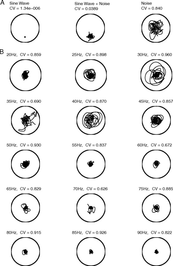
A, Phase portraits for a constant amplitude sine wave, a constant amplitude sine wave in noise, and noise only. B, Phase portraits of the data shown in Figure 3 for frequencies in the gamma band. Each portrait is for a 4 s period.

Test for visual response

For each experiment the LFP response to a blank stimulus (spontaneous activity) and an optimal drifting grating stimulus were recorded with 25 to 50 repetitions. An empirical probability density function (PDF) for the power at each frequency for the spontaneous activity was estimated by bootstrapping the mean of the Fourier transform of the spontaneous recordings. The power at each frequency of the stimulated data was estimated from the mean of the Fourier transform of the data. Those frequencies with stimulated power outside of the 95th percentile with respect to the spontaneous activity were considered significant.

Circular variance

The degree to which an oscillation is considered autocoherent can be characterized by the localization of the rotated phase portrait (described in Phase portraits and phase rotation). We used the circular variance (CV; Mardia, 1972) of the phase portraits as a statistic to quantify this localization and hence the phase coherence of the LFP signal at each frequency. The CV has values on [0,1]. The CV statistic, as used here, takes smaller values for ACOs and larger values for more random signals.

For the constant amplitude ACO null hypothesis described in Results, Phase portraits and phase rotation, the CV used to quantify the phase portraits has the form,

To quantify the autocoherence of the amplitude-modulated ACO null hypothesis described in Results, Null hypothesis II, the projection onto the second Fourier mode is used in the following formula,

The second mode is used in the amplitude-modulated case because the time varying amplitude, A(t), of the null-hypothesis model (Equation 18) is allowed to take on negative values. This results in an amplitude-modulated ACO having a phase portrait that lies along a line that passes through origin with values of the phase at ϕ − π.

Amplitude-modulated oscillations and heterodyning

A sinusoid whose amplitude is modulated may not necessarily be expected to have a phase portrait that is localized in a particular sector of the polar plot. Using the Fourier expansion of the amplitude modulation, we can express any arbitrary modulating signal as a series of phase shifted sinewaves,

Each of the products in Equation 12 can be expressed as a sum of two cosines using the trigonometric identity,

and are reduced to a series of constant amplitude sinusoids,

that will, under the CGT, exhibit localized phase portraits as described in Phase portraits and phase rotation. The expansion of an amplitude-modulated sinusoid in Equation 14 into a sum of constant amplitude sinusoids is referred to as ‘heterodyning’. The constant amplitude sinusoid sidebands in Equation 14 are called heterodynes and have symmetric amplitudes about the carrier frequency at the sum and difference frequencies of the carrier and component frequencies of the modulation. The phases of the heterodynes are also determined by Equation 14 to be the sum and difference of the phases of the carrier with the components of the modulation.

Modeling amplitude-modulated autocoherent oscillations

If the filters used in the Gabor transform to analyze the data had sufficiently narrow spectral resolution, the problem of detecting an amplitude-modulated ACO would simplify to detecting a series of constant amplitude ACOs that make up the sidebands. But to have filters with temporal resolution on the order of the burst seen in the LFP data, ∼100 ms (see Fig. 3D), the spectral width of the filters cannot be smaller than about 6 Hz, because of the uncertainty principle (see Eq. 5). Because of these limitations on the Gabor filters, an amplitude-modulated ACO cannot be detected by the constant amplitude ACO test described in Results, Null hypothesis I.

Figure 3.

Continuous Gabor transform (CGT) analysis of LFP data. A, The time course of a 4 s LFP recording (same example data as in Fig. 2A). B, Schematic diagram of continuous Gabor transform. C, The amplitude spectrum from the continuous Gabor transform of the time course in A.

To model an amplitude-modulated autocoherent oscillation, a symmetric modulation power spectrum centered on the carrier frequency ω₀ was fit to the significant frequencies in the gamma-band of the stimulated power spectra. The carrier frequency, ω₀, was estimated by calculating the center of mass of the significant frequencies in the gamma-band (20 to 90 Hz). The symmetric spectrum was fit by averaging the power in the sidebands on either side of the carrier. The modulation signal being modeled, A(t) of Equation 12, contains frequencies at the difference between the carrier, ω₀, and the sideband, ω_i. To avoid fitting noise, only frequencies that have power >1/3 of the carrier were included in the envelope. To generate a real-time series from the fitted symmetric modulation spectrum, the inverse Fourier transform was taken, with random phases assigned to the carrier frequency, ω₀, and to each component of the Fourier decomposition of A(t) (Equation 12) which correspond to the sets of symmetric sidebands in Figure 7A according to the heterodyning relation described above.

Figure 7.

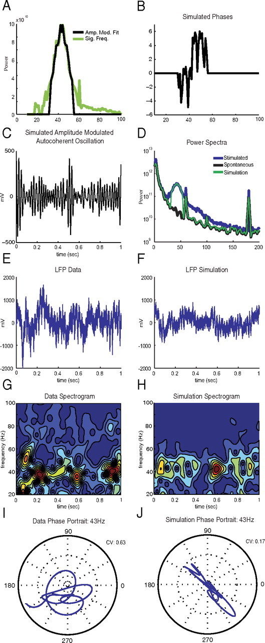
Simulation of null model: amplitude-modulated autocoherent oscillator from LFP data. A, Power of stimulated LFP data at frequencies significantly elevated from the spontaneous activity (green); power spectrum of the simulated amplitude-modulated ACO is a symmetric power spectrum fitted to the LFP data (black). B, Phase spectrum of simulated amplitude-modulated ACO. C, Simulated amplitude-modulated ACO signal, A(t), generated by the inverse Fourier transform of the spectra in A (black) and B. D, Power spectra of spontaneous activity of LFP data (black), stimulated LFP data (blue), and simulated null model: simulated amplitude-modulated ACO added to simulated spontaneous activity (green). E, Voltage time series of LFP data. F, Voltage time series of simulated null model: simulated amplitude-modulated ACO added to simulated spontaneous activity. G, Spectrogram of E. H, Spectrogram of F. I, Phase portrait of LFP data (subplot E) at the estimated carrier frequency. J, Phase portrait of simulated null model (subplot F) at the estimated carrier frequency.

Line noise filtering

In the data collected there was a strong line noise signal at 60 Hz associated with the alternating current of the electrical circuitry in the laboratory. Over the length of the recordings, the amplitude of the line noise was constant but its phase drifted. To filter out the line noise signal from the LFP recording, the amplitude of the 60 Hz signal line noise was estimated from the spectrum of the raw signal. This estimate was found by taking the Fourier transform of the entire record and interpolating the amplitude at 60 Hz from its neighboring values as an estimate of the 60 Hz component of the LFP signal. The amplitude of the line noise was assumed to be the difference between the interpolated amplitude and measured amplitude. This method effectively removed the line noise at 60 Hz in most cases, but it is still possible that higher harmonics (120 Hz and 180 Hz) of line noise were present in the data. As this study only examines the frequency band of 10 to 100 Hz, the harmonics did not pose a problem.

Results

Overview of study

In this study we have tested the idea that a deterministic oscillation, which may serve as a clock for the binding of stimuli across regions of the brain, underlies the gamma-band peak observed in the LFP recorded in V1. If it exists, this clock would supply a regular reference time for the precise temporal encoding of spikes. The gamma clock hypothesis is a prominent concept in studies of gamma activity, and for this reason it is important to submit it to rigorous statistical testing using in vivo data from cortex.

To assist the reader in navigating the study, we provide here a step-by-step summary. To begin, we review the extensive literature on the experimental and theoretical work that predicts the presence of a gamma clock oscillation in Oscillator models of the LFP (below). A demonstration of how traditional signal processing methods such as the power spectrum and spectrogram are not capable of discriminating nonautocoherent from autocoherent signals is presented in Need for statistical test of the ACO hypothesis versus intuition with an introduction to the new technique we have developed to measure the autocoherence of a signal. The cortical data are described in Local field potential data and Time-frequency analysis. In Null hypothesis I our first null hypothesis of a constant-amplitude ACO in noise is discussed. A description of the statistical test of this hypothesis is presented in Null hypothesis I: statistical tests. The results of the statistical test, in Null hypothesis I: test results, reject the constant amplitude ACO hypothesis and are plotted in Figure 6. The next model we consider, in Null hypothesis II, is an amplitude-modulated ACO in noise. In Null hypothesis II: statistical tests, we perform a statistical test of the amplitude-modulated ACO hypothesis. In Null hypothesis II: test results, the results of the statistical test reject the amplitude-modulated hypothesis and are plotted in Figure 8. To show that autocoherent neural signals exist in the brain and that our analysis is capable of detecting them, in Autocoherent oscillations in EEG data, we study an EEG recording that contains an alpha rhythm and find that it is autocoherent over several seconds. Finally, a discussion of the implications of the lack of autocoherence in gamma-band activity of cortex is presented in the Discussion.

Figure 6.

Statistical test of null hypothesis I: constant amplitude autocoherent oscillator (ACO). The differences between the CVs of the data at each frequency with significantly elevated power under visual stimulation for all 90 experiments and the simulated 99th percentiles of CV with respect to the constant amplitude ACO null model are shown. Differences greater than zero correspond to the rejection of the constant amplitude ACO hypothesis.

Figure 8.

Statistical test of null hypothesis II: amplitude-modulated autocoherent oscillator (ACO). Circular variances of the data with standard errors at the estimated carrier frequencies (red), and 99th percentile of the CV PDF of the simulated amplitude-modulated ACO null model (black).

Oscillator models of the LFP

An overwhelming amount of the theoretical neuroscience literature about the source of gamma-band spectral peaks has been concerned with the analysis of model networks that generate autocoherent oscillations. The reasons for this focus on autocoherent models were experimental evidence and also computational goals like the ‘clock’ theory of gamma oscillations.

Theorists hypothesized that oscillations in the LFP might be a ‘clock’ signal used to encode spikes temporally at precise times with respect to the phase of the LFP clock (Hopfield, 1995; Lisman and Idiart, 1995; Jefferys et al., 1996; Hopfield, 2004; Buzsaki and Draguhn, 2004; Fries et al., 2007). In these theories, regular rhythmic oscillations (which we call autocoherent oscillations) in the LFP were viewed as self-organizing emergent properties of the network. If different areas of the brain shared the same autocoherent LFP ‘clock’, the ‘clock’ oscillation could be used for ‘binding’ features of a stimulus to integrate information across many regions of the brain (Gray and Singer, 1989; Gray et al., 1989; Singer and Gray, 1995; Gray, 1999; Varela et al., 2001; Buzsaki, 2006).

The simplest proposed mechanism for the generation of a gamma clock signal is a population of cells each of which outputs a regular spike rate in the gamma band. For example, ‘chattering’ cells have been recorded in vivo from cat visual cortex that exhibit rhythmic firing in the 20 to 70 Hz range (Gray and McCormick, 1996).

Early mathematical models of networks of neurons found rhythmic oscillations in certain parameter regimes that were generated by feedback between inhibitory and excitatory cells (Freeman, 1975; Bressler and Freeman, 1980; Leung, 1982). But more recently most theoretical effort has been devoted to analyzing networks of inhibitory neurons as the source of gamma-band oscillations (Wang and Rinzel, 1992, 1993), and these inhibitory models generate autocoherent oscillations. A further development of the inhibitory network model was the clustering of subpopulations of inhibitory cells into groups that each generated autocoherent oscillations but were out of phase with each other. In this model the combined output of the various clusters generated an autocoherent oscillation with a frequency higher than each of the clusters (Golomb and Rinzel, 1994, van Vreeswijk, 1996). Models of synchronous and asynchronous states in mean field models of networks of neurons found that autocoherent oscillations depended on inhibitory coupling (Abbott and van Vreeswijk, 1993; van Vreeswijk et al., 1994; Gerstner, 1995; Gerstner et al., 1996).

In addition to earlier studies of gamma-band oscillations observed in visual cortex (Gray and Singer, 1989; Gray et al., 1989), gamma oscillations have also been recorded both in vivo (Bragin et al., 1995) and in vitro (Whittington et al., 1995) from rat hippocampus. Models of gamma oscillations in the hippocampus also used networks of inhibitory neurons to generate autocoherent oscillations that are thought to be functionally important (Whittington et al., 1995; Traub et al., 1996; Wang and Buzsaki, 1996; White et al., 1998; Ermentrout and Kopell, 1998; Chow et al., 1998; Kopell et al., 2000; Traub et al., 2000). Models in these studies of inhibitory networks generated autocoherent oscillations for either deterministic or noisy inputs whose autocoherent time-scales, the period of time over which the phase is conserved, were explicitly dependent on the time scale and properties of the external drive. A numerical simulation of a model network of inhibitory neurons is presented in the Appendix to demonstrate the autocoherent properties described in these studies.

Firing rate synchrony is another mechanism that has been proposed for the generation of autocoherent gamma-band oscillations. In models of firing rate synchrony, subthreshold membrane potentials of cells in the network exhibited rhythmic oscillations but cells fired spikes irregularly. However, individual neurons fired spikes preferentially at the peaks of the membrane potential oscillation. In this class of models, the spiking output of individual cells did not exhibit periodic firing, but the network-averaged firing rate exhibited an autocoherent gamma-band oscillation (Kopell and LeMasson, 1994; Brunel and Hakim, 1999; Tiesinga and Jose, 2000; Brunel and Wang, 2003; Geisler et al., 2005; Brunel and Hansel, 2006).

The ACO hypothesis, in the form of either spike or membrane potential synchrony, has been widely cited and is very influential in the experimental literature on gamma-band oscillations. The theoretical concept of emergent autocoherent oscillations has been cited in experimental studies of the hippocampus (Penttonen et al., 1998; Fisahn et al., 1998; Traub et al., 2000; LeBeau et al., 2002; Mikkonen et al., 2002; Csicvari et al., 2003; Vida et al., 2006; Mann and Paulsen, 2007; Montgomery and Buzsaki, 2007), visual cortex (Gray and Singer, 1989; Zaksas and Pasternak, 2006), prefrontal cortex (Compte et al., 2003; Durstewitz and Gabriel, 2007), and somatosensory cortex (Cardin et al., 2009), among others.

To demonstrate that autocoherent oscillations do exist in neural data and therefore that our statistical test of the ACO hypothesis is capable of having both positive and negative outcomes, an example of EEG data containing an alpha rhythm (11 Hz oscillation) is analyzed in Autocoherent oscillations in EEG data using our new statistical method (described in Time-frequency analysis to Null hypothesis II). In the EEG data there was a clear autocoherent oscillation that lasted for 3 s (roughly 30 oscillations of the alpha rhythm). The EEG results established that the ACO hypothesis is a biologically plausible claim worth testing rigorously and that our method is capable of detecting ACOs when they exist.

It is possible to conceive of models that generate gamma-band peaks in which the frequency components are not autocoherent. Such stochastic models are considered in the Discussion. Testing cortical data for autocoherence is an important goal for experiments and data analysis because determining whether or not the data are autocoherent can decide between classes of models of the cerebral cortex and other brain areas.

Need for statistical test of the ACO hypothesis versus intuition

It is commonly thought, based on intuition, that the autocoherence of a signal can be diagnosed by visual inspection of the time series, but this intuition is incorrect, as demonstrated in Figure 1. For example, plotted in Figure 1A is a simulated, amplitude-modulated ACO of the form

where the phase ϕ₀ is constant in time and ω₀ is set to 40 Hz and A(t) is the sum of three Gaussians with peaks roughly centered at 0.2 s, 1.2 s, and at 2.9 s. Figure 1B is a plot of a simulated nonautocoherent signal, of the form

where ω₀ is again equal to 40 Hz, each of the three individual bursts' amplitudes, given by the Gaussian A_i functions, are separated in time (A₁(t) centered at 0.2s, A₂(t) centered at 1.2 s, and A₃(t) centered at 2.9s) and the phases of the separate bursts, ϕ_i, are unrelated. It is not possible to discriminate between the autocoherent (Fig. 1A) and nonautocoherent oscillation (Fig. 1B) by eye, even in this noiseless case. In Figure 1, C and D, the two kinds of oscillations are added to simulated spontaneous V1 LFP activity, generated using the power spectra of data used in this study (Null hypothesis I: statistical tests) to recreate the noise that is commonly present in LFP recordings. In Figure 1, E and F, the power spectra, and in Figure 1, G and H, the spectrograms, of the two kinds of oscillations are plotted, after the two oscillatory signals were added to the simulated spontaneous LFP activity. These examples of simulated LFP signals demonstrate that it is not possible to discriminate an autocoherent signal from a time-varying phase signal by a visual comparison of the time series, the power spectra, or the spectrograms. For this reason we developed a new method of data analysis to determine the autocoherence of a signal. The new method examines the time dependence of the phase of the signal. In Figure 1, I and J, the phase portraits (Materials and Methods, Phase portraits and phase rotation) at 40 Hz of the two example signals (autocoherent and drifting phase) are plotted. The phase portraits are parametric plots (time increasing along the curve) with phase represented by the angle and the amplitude by the radius. For the autocoherent oscillation (Figure 1I) each burst of activity away from the origin has the same phase (azimuthal angle), whereas in the case of the signal that has a phase that varies with time (Figure 1J) each burst of activity has a different phase angle. The difference between the two signals can be understood by studying their phase portraits.

Figure 1.

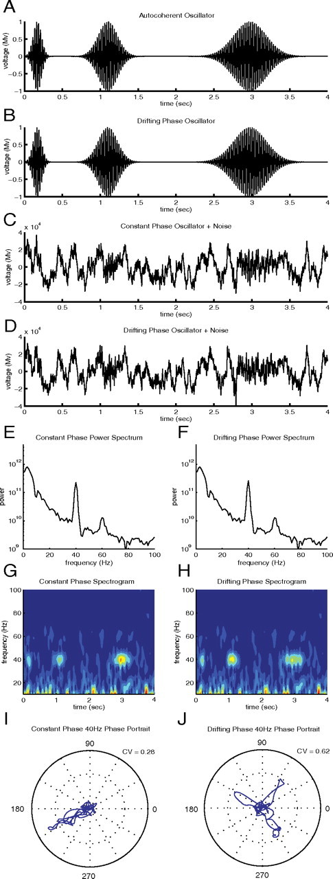
A, Amplitude-modulated autocoherent sine wave at 40 Hz. B, Amplitude-modulated drifting phase sine wave at 40 Hz. C, Amplitude-modulated autocoherent sine wave at 40 Hz added to simulated spontaneous V1 LFP activity. D, Amplitude-modulated drifting phase sine wave at 40 Hz added to simulated spontaneous V1 LFP activity. E, Power spectrum of signal C. F, Power spectrum of signal D. G, Spectrogram of signal C. H, Spectrogram of signal D. I, Phase portrait at 40 Hz of signal C. J, Phase portrait at 40 Hz of signal D.

Local field potential data

The local field potential (LFP) is an extracellular voltage measurement that characterizes the local network activity of the population of neurons in the neighborhood of the measuring electrode (approximately 10² to 10³ neurons) and is defined as the low frequency (≤250 Hz) portion of the raw field potential. Specifically, the LFP signal measures the current flow attributable to synaptic activity, whereas the higher frequency components of the raw data are related to action potentials (Kruse and Eckhorn, 1996; Logothetis et al., 2001; Buzsaki, 2006).

The LFP data analyzed here were obtained by recording with extracellular microelectrodes in macaque V1 cortex, in monkeys lightly anesthetized with the opioid sufentanil. LFP spectra and spectrograms were measured during a baseline blank (no stimulus) and also during visual stimulation with a high-contrast drifting grating pattern (using a monitor with a 100 Hz refresh rate) at the ‘preferred’ orientation for maximal response (further experimental details described in Materials and Methods, Visual stimulation). The LFP response to a blank stimulus was recorded for 1 s and the grating pattern was shown for 2 or 4 s, both with 25 to 50 repetitions depending on the trial. The data are from 90 experiments in two monkeys where LFPs were recorded with multielectrode arrays of seven electrodes. Voltage data were sampled at a rate of 25 kHz. Data from the electrode with the largest response to the visual stimulus were selected for analysis, as these give the largest signal-to-noise ratio for our statistical tests. The 60 Hz line noise signal was filtered out of the LFP recordings as described in Materials and Methods, Line noise filtering. An example of a 4 s LFP recording under visual stimulation is plotted in Figure 2A and its power spectrum in Figure 2B. The power spectra were computed using a multitaper analysis (Percival and Walden, 1993) with a concentration bandwidth of 1 Hz and averaged over repeated identical stimuli.

Figure 2.

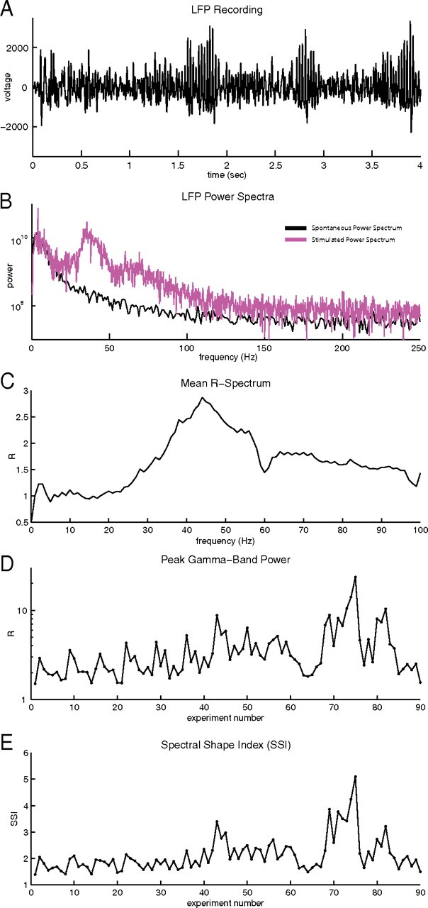
Gamma-Band power spectrum from 90 experiments A, The time course of a 4 s LFP during visual stimulation by a drifting grating. B, Power spectra of the LFP: spontaneous LFP spectrum (black); LFP spectrum of the response to a drifting grating stimulus (magenta) from A. C, R-spectrum of the data from 10 to 100 Hz averaged over all 90 experiments. D, Peak value of the R-spectrum in the gamma-band for each experiment. E, Spectral shape index (SSI) for each experiment. The slow trend upwards in D and E are not meaningful and probably reflect increasing skill of the experimenters.

In all 90 experiments, localized elevated power was observed in the gamma-band during visual stimulation. Plotted in Figure 2C is the LFP R-spectrum (see Materials and Methods, R-Spectrum and spectral shape index) averaged over all 90 experiments studied. The R-spectrum is the power spectrum of the visually driven response normalized by the baseline spontaneous spectrum. The averaged R-spectrum shows a clear ‘bump’ in the gamma-band that begins near 20 Hz, peaks between 35 and 50 Hz, and decreases gradually to 100 Hz. After filtering, the line noise from the experiment setup (see Materials and Methods, Line noise filtering) has a stronger relative signal in the spontaneous spectrum compared to the stimulated spectrum, resulting in a narrow notch about 60 Hz in the averaged R-spectrum in Figure 2C. This notch does not effect the conclusions of the study as the line noise was well separated from the gamma-band peak power. Plotted in Figure 2D is the maximum or peak value of the R-spectrum in the gamma-band for each experiment. All visually driven LFPs had a peak gamma-band power larger than the spontaneous power (R > 1), meaning the LFP gamma-band power was strongly visually driven by the drifting gratings (cf. Henrie and Shapley, 2005). The sharpness of the gamma-band ‘bump’ in the visually-driven power spectrum was quantified by comparing the peak power in the gamma-band in relation to the surrounding frequencies with a spectral shape index (SSI) (see Materials and Methods, R-Spectrum and spectral shape index). The SSI is computed to determine whether each experiment displayed localized elevated gamma-band power (narrow ‘bump’; SSI > 1) or broad-band elevated power at all frequencies (broad ‘bump’; SSI < 1). In this study the characteristics of gamma activity are examined. As such, experiments that displayed a localized narrow ‘bump’ of gamma-band power were most useful. Plotted in Figure 2E are the SSIs evaluated for each experiment. For all experiments analyzed, the SSI > 1, indicating that there was a localized peaked ‘bump’ of power in the gamma-band.

Time-frequency analysis

We used a time-frequency analysis to examine the temporal evolution of LFP data at each frequency. Similar analyses have previously been used to study the temporal structure of brain activity recorded in EEG (Makeig, 1993; Herrmann et al., 2004), LFP (Pesaran et al., 2002), and have been described as a general method for studying event-related activity in neural signals (Sinkkonen et al., 1995; Mitra and Pesaran, 1999; Hurtado et al., 2004). The continuous Gabor transform (CGT) is the convolution of an enveloped complex plane wave ψ with the time series being examined (see Materials and Methods, Continuous Gabor transform). The CGT is a function of t, the time point at the center of the convolution, and ω₀, the frequency of the underlying wave of the transform (shown schematically in Fig. 3B). Scale varying wavelets, whose width in the time domain dilates with increasing scale (decreasing frequency), become too coarse in the time domain at low frequency and too broad in the frequency domain at higher frequencies for this study. To avoid the problems associated with the scale representation of wavelet transforms, we used the Gabor transform because its fixed time scale preserves the relationship to frequency.

Plotted in Figure 3C is the CGT amplitude spectrum of the LFP recording shown in Figure 3A. In comparing the amplitude spectrum with the LFP time series, the three bursts of activity in Figure 3A at times t = 1.75 s, 2.8 s, and 3.75 s correspond to high-amplitude events in Figure 3C. It is clear that the CGT is capable of capturing the time evolution of the LFP recording. From inspection of Figure 3C, the LFP signal has large bursts of activity on the scale of ∼100 ms with power concentrated mainly near 35 Hz and with a smaller peak at 70 Hz. The spectral peak between 35 Hz and 45 Hz and the 100 ms time scale were characteristics common to all LFP recordings analyzed here.

Null hypothesis I: constant amplitude autocoherent oscillator

The first null hypothesis we consider is that the increased gamma-band power seen in the LFP power spectrum is the result of a constant amplitude autocoherent oscillation of the local neuronal network that becomes active under visual stimulation. Autocoherence in this case means that at a particular frequency the LFP can be modeled as a sine wave of constant phase and amplitude added to noise,

where A and ϕ are time-independent.

In the event there were multiple autocoherent oscillators in the network operating at the same frequency, the waveforms of the different oscillations would be summed when recorded with an electrode. The sum of many different constant-phase sine waves at the same frequency is a single sine wave that our method would detect as an autocoherent oscillation.

One can examine the autocoherence at a particular frequency by studying plots of the rotated phase portrait (see Materials and Methods, Phase portraits and phase rotation). When a signal has large amplitude bursts at a particular frequency, for example as seen in the LFP data in Figure 2A, the phase portrait will show a large amplitude excursion away from the origin at that frequency as shown in Figure 1, I and J. This kind of phase portrait is illustrated in Figure 4 for idealized systems in 4A and for real LFP data in 4B. The phase of the constant amplitude sine wave appears as a single point in the phase portrait (Fig. 4A, left). If noise is added to the sine wave, the rotated phases do not all fall on a single point (Fig. 4A, middle) but remain localized in a common sector of the polar plane rather than exploring all quadrants as is done by the phases of a noise signal (Fig. 4A, right).

Phase portraits for the LFP data shown in Figure 3 are plotted in Figure 4B at frequencies in the gamma-band from 20 to 90 Hz. If the LFP contained constant amplitude autocoherent oscillations, as in the null hypothesis, the activity in the phase portrait should have clustered in a common sector of the phase portrait. The phase portraits of the peaks in the spectral power at 35 Hz and 70 Hz (Fig. 3A,C) show high amplitude (large radius) events that correspond to the bursts discussed in Time-frequency analysis. In the 35 Hz and 70 Hz phase portraits the three bursts seen in the LFP time series (Fig. 3A) and the CGT spectrum (Fig. 3C) are visible in the three ‘loops’ away from the origin. These bursts occupied different sectors of the phase portrait, and therefore the signal was not autocoherent.

We used circular variance (CV; see Materials and Methods, Circular variance) as a statistic to quantify the coherence of an oscillation or, equivalently, localization of the trajectories of the phase portraits. The CV varies from zero to one and measures how tightly clustered the points are in phase angle. A CV close to zero corresponds to all points having similar phases and, for our purposes, a more autocoherent oscillation. A CV near one indicates that the different points in time have different phases and implies a nonautocoherent signal with a time-varying phase. The CV is normalized by the average amplitude of the oscillation and is dimensionless. One can use the dimensionless CV index to compare the coherence of oscillations of different frequencies and power. The CV of the phase portraits in Figure 4 are listed above the plots at each frequency. The CVs of the 35 Hz and 70 Hz oscillations in the LFP data from V1 were large, 0.69 and 0.63, respectively, a result which suggests there were not autocoherent oscillations at these two frequencies.

Null hypothesis I: statistical tests

We have shown visually and using the CV statistic that the oscillations seen in the data in Figures 3 and 4 were not autocoherent. But to examine systematically all 90 experiments and to determine quantitatively whether autocoherent oscillations were present as proposed by the null hypothesis, a statistical test had to be performed. The first step was to identify which frequencies of the LFP had significantly elevated power under visual stimulation, a step which was done as described in Materials and Methods, Test for visual response.

We devised a Monte Carlo-type statistical test to determine whether autocoherent oscillations were present in the visually-driven LFP signal. For all 90 experiments we performed the following simulations whose procedure is described schematically in Figure 5. A test was evaluated at all frequencies between 10 and 100 Hz that had significantly elevated power under stimulation. At a particular frequency, the null-hypothesis model assumes that the increase in power at that frequency under visual stimulation had a constant amplitude and fixed phase and was summed with background noise. The background noise was simulated by taking the average amplitude spectrum of the spontaneous LFP data, from 1 to 250 Hz, assigning random phases to each frequency and taking the inverse Fourier transform. A constant amplitude ACO of the form (Equation 17) was added to the simulated background noise. The amplitude of the oscillator, A, was found by taking the square root of the difference between the stimulated and background power spectra at the frequency being tested; the phase, ϕ, was chosen randomly. The CGT (Mallat, 1999; see Materials and Methods, Continuous Gabor transform) of the simulated signal was taken, and the CV of the phase portrait was computed. This simulation procedure was repeated 1000 times to generate a probability density function (PDF) of the values of the CV for the null-hypothesis model.

Figure 5.

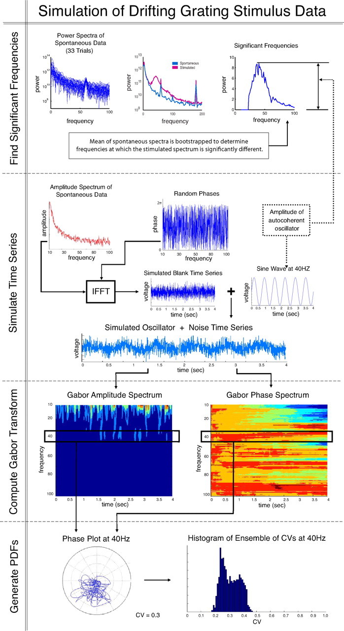
Flow chart for the generation of the simulated CV PDF for the constant amplitude ACO null hypothesis.

Null hypothesis I: test results

The null hypothesis of a constant amplitude ACO was rejected at all frequencies tested, between 10 and 100 Hz. In particular, there was no evidence for an ACO in the gamma band where the visually driven spectral power peaked. Plotted in Figure 6 are the differences between the CVs of the data at each frequency and the simulated 99th percentiles of the CV of the constant amplitude ACO, the null-hypothesis model. The differences between data and the null-hypothesis model are plotted in Figure 6 at all frequencies with significantly elevated power under visual stimulation for all 90 experiments. The differences were greater than zero for all experiments at all frequencies, with the exception of 60 Hz where a strong line noise signal was still present after filtering, and 100 Hz which was the refresh rate of the computer monitor used to present the visual stimulus in the experiments. That the CVs of the data were larger than the 99th percentile of the null-hypothesis model reveals that the V1 gamma-band data were significantly less autocoherent than a constant amplitude ACO.

In the range of frequencies of the gamma-band near 40 Hz, where the elevated power in the data was centered, the difference between the CV of the data and of the constant amplitude ACO (denoted ‘sample average’ in Fig. 6) had its largest values, indicating that the oscillations in this frequency band of interest were particularly nonautocoherent. This occurred because the gamma band was the region of the LFP spectrum where the LFP had the largest elevation of power in response to the visual stimulus. To fit the LFP data in the gamma band, the ACO in the null model had to have a larger signal-to-noise ratio than at other frequencies, hence the phase of the ACO sine wave dominated the phase trajectory and led to a lower CV value. This caused the larger difference between the data CV and null CV in the gamma band. The CV values of the LFP data from V1 were relatively constant across the frequencies analyzed which meant the CV difference was higher when the signal-to-noise in the null-hypothesis model rose.

From Figure 6 we conclude that the null hypothesis of a constant amplitude ACO was not supported by the V1 data analyzed here and that constant amplitude ACOs did not occur in macaque V1, even when there were strong gamma-band spectral peaks.

Null hypothesis II: amplitude-modulated autocoherent oscillator

The constant amplitude ACO hypothesis, rejected in Null hypothesis I, is the simplest type of oscillatory response expected from a deterministic system. Another type of oscillation consistent with the ACO hypothesis is an amplitude-modulated ACO of the form

where the modulation, A, is now a function of time, but ϕ₀ is still time-independent and the carrier frequency, ω₀, is assumed to be in the range of the gamma-band peak seen in the data (30 to 50 Hz). Using a Fourier decomposition of A(t) and trigonometric identities we showed in Materials and Methods, Amplitude-modulated oscillations and heterodyning that an amplitude-modulated ACO can be expressed as a sum of constant amplitude ACOs (for ω₀ ≠ 0) through the heterodyning relation. Heterodyning is an effect where an amplitude-modulated sinusoid can be expressed as a carrier friequency, ω₀, with symmetric sidebands at frequencies equal to the sum and difference of the carrier frequency and modulation frequencies and phases of the sidebands equal to the sum and difference of the phase of the carrier and modulation phases.

Null hypothesis II: statistical tests

To provide intuition about amplitude-modulated ACOs, we simulated an example as described in Materials and Methods, Modeling amplitude-modulated autocoherent oscillations. The simulation is shown in Figure 7A–C, where the fitted symmetric modulation spectrum is shown in black in Figure 7A, the random phase spectrum is plotted in Figure 7B, and the resulting real-time series after taking the inverse Fourier transform is shown in Figure 7C.

A statistical test similar to that described in Null hypothesis I: statistical tests for the constant amplitude ACO hypothesis was used for the amplitude-modulated ACO hypothesis. Unlike the constant amplitude test, the amplitude-modulated case was only tested at the carrier frequency, ω₀, rather than all significant frequencies. To simulate the amplitude-modulated ACO-null model, the modulation signal was fit nonparametrically to the power spectra of the data as described in Materials and Methods, Modeling amplitude-modulated autocoherent oscillations, and multiplied by a fixed phase sinewave as in Equation 18. This simulated null-hypothesis oscillation was then added to simulated spontaneous activity generated in the same manner as for the constant amplitude-null hypothesis (Null hypothesis I: statistical tests). For example, the power spectra of the spontaneous, stimulated, and simulated amplitude-modulated ACO null-hypothesis model are shown in Figure 7D, where the simulated null-hypothesis model only includes the power spectrum peak in the gamma band and not the complete stimulated spectrum. In Figure 7, E and F, are plotted the time series, and in Figure 7, G and H, the spectrograms of the data and the simulated null model, respectively. The difference between the autocoherence of the data and the simulation became clear when the phase portraits at the carrier frequency (here 43 Hz) (plotted in Fig. 7I,J) were compared. The phase portrait of the data had a wandering shape corresponding to a time-varying phase signal whereas the phase portrait of the simulated signal fell along a line that signifies the presence of an amplitude-modulated ACO (see Materials and Methods, Amplitude-modulated oscillations and heterodyning). As in the constant amplitude case, the CV (Materials and Methods, Circular variance) was used to quantify this difference. A simulated PDF of the CV values for the null hypothesis was generated in the similar manner as for the constant amplitude case (Fig. 5) but with the simulation of the constant amplitude ACO replaced with the amplitude-modulated simulation. The hypothesis was tested at the carrier frequency, ω₀ of Equation 18, for each experiment by comparing the CVs of the data to the 99th percentile of the PDF of the simulated null-hypothesis CV.

Null hypothesis II: test results

The results of the amplitude-modulated ACO null hypothesis are shown in Figure 8. In Figure 8 the CVs of the data are plotted with their standard errors along with the 99th percentile of the CV for the null-hypothesis model for each experiment. The CVs of the data, including the measurement errors, were all in excess of the 99th percentile of the null hypothesis for all 90 experiments tested. These results reject the amplitude-modulated ACO hypothesis as an explanation for the observed elevated gamma-band power spectra in macaque V1.

Autocoherent oscillations in EEG data

Our focus in this article has been on gamma-band activity, but we include here an example of the analysis of alpha rhythms in human EEG to make the point that it is possible for some brain activity to be much more autocoherent than the gamma-band activity we analyzed above, and that our analysis will find the autocoherence if it exists. An example of an autocoherent oscillation in EEG data is plotted in Figure 9. The autocoherent oscillation lasted for 3 s over the course of ∼30 cycles. The EEG recording, bandpassed filtered from 5 to 50 Hz, is plotted in Figure 9A. The power spectrum of the recording is plotted in Figure 9C with a peak in the alpha band at 11 Hz. The phase portrait at 11 Hz of the EEG recording in Figure 9A is plotted in Figure 9B. The phase trajectory of the alpha oscillation in the phase portrait was largely confined to the region of 150 to 240 degrees with a CV value of 0.25 (see Materials and Methods, Circular variance) indicating an autocoherent signal. The mean phase is shown by the black arrow in Figure 9B. An autocoherent 11 Hz sine wave whose phase is given by the mean of the phase portrait and whose amplitude is given by the amplitude coefficients of the Gabor transform of the EEG at 11 Hz is overlayed on the EEG data in Figure 9A. The EEG data and the autocoherent sine wave have corresponding phases for most of the 3 s record with occasional periods where the 11 Hz amplitude temporarily fades (during the period of 1.4 to 1.75 s) and then reappears with the same phase. This EEG example shows that persistent amplitude-modulated autocoherent oscillations exist in neural data, and our method can identify them when they are present in data. Although this alpha rhythm has been shown to be autocoherent, cortical gamma-band activity is very different because of the absence of autocoherence in gamma.

Figure 9.

A, Time course of a 3 s EEG recording exhibiting an autocoherent oscillation at 11 Hz (black), and fitted autocoherent alpha oscillation (green). B, Phase portrait at 11 Hz of the EEG recording plotted in A (blue), and mean phase of the 11 Hz trajectory (black arrow). C, Power spectrum of EEG recording plotted in A.

Discussion

The results of our new time-frequency analysis of V1 local field potentials (LFPs) reject the hypothesis that gamma-band spectral peaks in the LFP of visually driven macaque V1 LFP data (Fig. 3A) can be modeled as a constant-amplitude ACO (Equation 17) or as an amplitude-modulated ACO (Equation 18). In the data examined here a gamma-band peak in power is induced using a drifting grating stimulus, as has been shown to occur in previous work on gamma activity in V1 (Bauer et al., 1995; Frien et al., 2000; Ray and Maunsell, 2009). We conclude that elevated gamma-band energy in V1 is not the result of emergent deterministic, harmonic, or relaxation, oscillations investigated in the modeling studies referenced in Results, Oscillator models of the LFP. Thus, the present results rule out a class of theoretical models for gamma activity in the V1 network.

The results in this article call into question the idea that the gamma oscillation in V1 is operating as a ‘clock’ signal for the precise temporal encoding of visual information. If there is a ‘clock’ mechanism present in V1 gamma activity, the period of time over which it supplies reliable timing (time over which the phase of the oscillation is conserved) is not set by the time-scale of the stimulus but may have some intrinsic time-scale attributable to internal dynamics of the cortical network itself. This intrinsic time scale must be much shorter than the duration of the visual stimulus we used, on the order of 2 to 4 s. Similarly, if gamma activity is involved in the ‘binding’ of stimulus features across different regions of the brain by gamma, the period of time over which the brain can synchronize different areas must be very brief and is also not determined by the time scale of the stimulus being processed.

Theoretical models of gamma oscillations predict autocoherent oscillations whose time-scales are set by the properties of the external drive to the network (see Results, Oscillator models of the LFP). Applied to the measurements in this study, these models would predict that for a constant visual stimulus (drifting grating stimulus) the time-scale of autocoherent oscillations seen in the LFP should persist for the length of the time the stimulus is presented (2 to 4 s). Previous measurements of gamma activity from hippocampus in rat, described in Results, Oscillator models of the LFP, were recorded in vitro in slices rather than in vivo as in the experiments analyzed here. It is possible that the oscillations seen in slice, driven with a tonic external drive, do generate autocoherent oscillations, but the work here shows that for in vivo V1 networks this is not the case.

The alpha rhythm, analyzed in Results, Autocoherent oscillations in EEG data, exhibited an autocoherent oscillation at 11 Hz. It is possible that lower frequency oscillations such as the alpha (8 to 12 Hz) and theta (6 to 10 Hz) rhythms may be autocoherent. The work of Wang and Rinzel (1992, 1993) was originally motivated as models of spindle rhythms with a frequency of 7 to 14 Hz. Their model is not an accurate model of gamma activity in V1 but may be a useful model of alpha and theta rhythms.

For a model to generate bursts at arbitrary times of arbitrary length, as seen in the data, a fundamentally different type of nondeterministic model must be used. In the theoretical models discussed in Results, Oscillator models of the LFP, noise in the system is viewed as something that may obscure synchronous firing that allows the system to oscillate autocoherently. Rather than treating noise as a corrupting factor, we believe noise is essential to the generation of the gamma-band peak and should be treated as a leading order term in any mathematical model of gamma oscillations. To accommodate the random aspects of the timing and duration of bursts seen in the data, any biologically accurate mathematical model should include a random variable term representing noise. Doing this will necessarily cause the system to be modeled stochastically rather than the deterministic approaches of the previous theoretical studies of gamma-band ‘oscillations’.

Although this study has shown that the ACO model does not fit the data from V1, there is structure in the data in the form of bursts of activity concentrated in particular frequencies of the gamma band. A model that can produce the peaked, elevated gamma-band power spectra recorded in V1 and that includes a central role for noise is a resonant stochastic filter. Henrie et al. (2005) and Kang et al. (2009) found that a stochastic resonant network model of V1 with recurrent connections to extrastriate cortex has a resonant response in the gamma-band. In this model the network is viewed as a resonant stochastic oscillator with a stable state for noiseless inputs corresponding to the quiescent periods (low amplitude) of the LFP data (see Fig. 3B). When noise is added to the system during visual stimulation, from feed-forward and recurrent inputs, the network is randomly excited into short high-energy bursts of excitation at a resonant frequency centered in the gamma band (see also similar ideas expressed in Rennie et al., 2000). In a resonant stochastic oscillator model, the phase associated with each burst is independent, and the signal is not autocoherent for the length of the period of stimulation. The varying phases associated with the independent bursts of activity generate a broad peak in the power spectrum of the LFP, a peak centered on the resonant frequency of the network, as seen in the data presented here (Fig. 2B). The gamma-band resonance in the model of Kang et al. (2009) is a consequence of the structure of the model network they considered: a recurrent excitatory-inhibitory network in which synaptic inhibition and excitation both have short time constants, with the inhibitory time constant slightly slower than that of excitation. Networks with this functional connectivity have been proposed before to explain cortical sharpening of selectivity (for example, Kang et al., 2009). The presence of gamma-band resonance in such networks may be a by-product of their dynamics, but it may also enhance their sensory function. Our future research on the elevated gamma-band response to visual stimuli will focus on testing whether the data are consistent with such a stochastic resonant oscillator model.

An alternative to the stochastic model we favor, which also generates an irregular, nonautocoherent activity, is a model of network activity with finely tuned parameters such that the network oscillates chaotically. Models of neuronal networks that exhibit chaotic oscillations have been explored by Hansel and Sompolinsky (1996) and Battaglia et al. (2007) as possible mechanisms for generating nonautocoherent network activity.

We found that gamma activity is not autocoherent on the time-scale of the visual stimulus (2 to 4 s). However, on shorter time-scales, individual bursts of activity may be autocoherent. Spatially coherent bursts of gamma-band activity have been found in the rat hippocampus with a time-scale of ∼100 ms (Montgomery and Buzsaki, 2007; Montgomery et al., 2008). Further work on autocoherence in LFP data should include a study to determine the intrinsic internal autocoherent time scale of individual bursts of gamma activity seen in the data. The time-frequency analysis developed here could be used for such an analysis. Also, as described in the introduction, gamma-band spectral peaks have been observed in many other regions of the brain. With the development of the new time series analysis presented in this paper, data from other brain regions could be examined to determine the autocoherence of LFP activity throughout the brain.

Appendix

Autocoherence analysis of inhibitory network model

A model of 10 inhibitory integrate and fire neurons with a constant excitatory drive was simulated numerically to demonstrate the deterministic clock mechanism referred to in Results, Oscillator models of the LFP. The details of the conductance-based model used for the simulation, and the parameters used, are described in Tao et al. (2004). The model was time stepped using a fourth order Runge-Kutta method (Press et al., 1992), and the neurons were connected all-to-all with equal strength. The network was integrated for 5 min; it quickly (<50 ms) locked into a regular oscillation that persisted for the duration of the simulation. To model the influence this inhibitory network would have on the membrane potential of an excitatory neuron, the population average time course was convolved with an inhibitory synaptic conductance kernel (see Tao et al., 2004). A 500 ms excerpt of the population average voltage time course, smoothed with the synapse's kernel, is plotted in Figure 10A.

Figure 10.

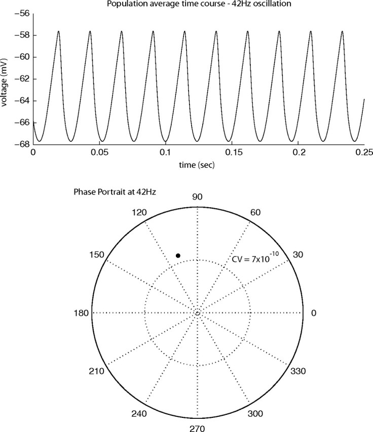
Output of the numerical simulation of a model network of 10 inhibitory neurons connected all-to-all. A, Population average voltage time course convolved with an inhibitory synaptic conductance kernel. B, Phase portrait and circular variance at 42 Hz of the time course plotted in A.

This inhibitory model generates a regular clock oscillation and is a simplified version of the same network mechanism proposed by previous theorists to be the source of the gamma-band peak seen in cortical LFP data as reviewed in Results, Oscillator models of the LFP. A fundamental aspect of this model is that the connections between the inhibitory cells in the network cause each of the cells to fire more slowly than they would in isolation. In this network the inclusion of inhibitory connections slows the network oscillation from 70 Hz down to 42 Hz, which is within the gamma-band frequency range (20 to 90 Hz). The autocoherence of the model's output was calculated using the same technique as described in Results, Null hypothesis I. The phase portrait at 42 Hz of the time course plotted in Figure 10A is plotted in Figure 10B. The CV of the model's output is 7 × 10⁻¹⁰, which indicates the model is outputting a perfect clock signal. If this inhibitory network clock mechanism were the source of the gamma activity seen in V1, strong autocoherent signals should have been present in the LFP data analyzed here, by the following argument. It is reasonable to suppose that the excitatory cells are getting added random noise and that this then would be added to the inhibitory clock signal in the LFP. The inhibitory clock signal with its 0 CV value would be equivalent to the continuous sinusoid we considered in Null Hypothesis 1 in Results, Null hypothesis I. The analysis in the article that rejected Null Hypothesis 1 therefore also rejected the hypothesis that inhibitory clock signals were the source of the gamma-band peaks in the LFP.

References

- Abbott LF, van Vreeswijk C. Asynchronous states in a network of pulse-coupled oscillators. Phys Rev E. 1993;48:1483–1490. doi: 10.1103/physreve.48.1483. [DOI] [PubMed] [Google Scholar]
- Bartos M, Vida I, Jonas P. Synaptic mechanisms of synchronized gamma oscillations in inhibitory interneuron networks. Nature Rev Neurocsci. 2007;8:45–56. doi: 10.1038/nrn2044. [DOI] [PubMed] [Google Scholar]
- Battaglia D, Brunel N, Hansel D. Temporal decorrelation of collective oscillations in neural networks with local inhibition and long-range excitation. Phys Rev Let. 2007;99:238106. doi: 10.1103/PhysRevLett.99.238106. [DOI] [PubMed] [Google Scholar]
- Bauer R, Brosch M, Eckhorn R. Different rules of spatial summation from beyond the receptive field for spike rates and oscillation amplitudes in cat visual cortex. Brain Res. 1995;669:291–297. doi: 10.1016/0006-8993(94)01273-k. [DOI] [PubMed] [Google Scholar]
- Bragin A, Jando G, Nadasdy Z, Hetke J, Wise K, Buzsaki G. Gamma (40–100 Hz) oscillation in the hippocampus of the behaving rat. J Neurosci. 1995;15:47–60. doi: 10.1523/JNEUROSCI.15-01-00047.1995. [DOI] [PMC free article] [PubMed] [Google Scholar]
- Bressler SL, Freeman WJ. Frequency analysis of olfactory system EEG in cat, rabbit, and rat. Electroencephalogr Clin Neurophysiol. 1980;50:19–24. doi: 10.1016/0013-4694(80)90319-3. [DOI] [PubMed] [Google Scholar]
- Brunel N, Hakim V. Fast global oscillations in networks of integrate-and-fire neurons with low firing rates. Neural Comput. 1999;11:1621–1671. doi: 10.1162/089976699300016179. [DOI] [PubMed] [Google Scholar]
- Brunel N, Wang XJ. What determines the frequency of fast network oscillations with irregular neural discharges? I. Synaptic dynamics and excitation-inhibition balance. J Neurophysiol. 2003;90:415–430. doi: 10.1152/jn.01095.2002. [DOI] [PubMed] [Google Scholar]
- Brunel N, Hansel D. How noise affects the synchronization properties of recurrent networks of inhibitory neurons. Neural Comput. 2006;18:1066–1110. doi: 10.1162/089976606776241048. [DOI] [PubMed] [Google Scholar]
- Buzsaki G. Rhythms of the Brain. Oxford UP: 2006. [Google Scholar]
- Buzsaki G, Chrobak JJ. Temporal structure in spatially organized neuronal ensembles: a role for interneuronal networks. Curr Opin Neurobiol. 1995;5:504–510. doi: 10.1016/0959-4388(95)80012-3. [DOI] [PubMed] [Google Scholar]
- Buzsaki G, Draguhn A. Neuronal oscillations in cortical networks. Science. 2004;204:1926–1929. doi: 10.1126/science.1099745. [DOI] [PubMed] [Google Scholar]
- Cardin JA, Carlen M, Meletis K, Knoblich U, Zhang F, Deisseroth K, Tsai LH, Moore C. Driving fast-spiking cells induces gamma rhythms and controls sensory responses. Nature. 2009;459:663–667. doi: 10.1038/nature08002. [DOI] [PMC free article] [PubMed] [Google Scholar]
- Chow CC, White JA, Ritt J, Kopell N. Frequency control in synchronized networks of inhibitory neurons. J Comput Neurosci. 1998;5:407–420. doi: 10.1023/a:1008889328787. [DOI] [PubMed] [Google Scholar]
- Compte A, Constantinidis C, Tegner J, Raghavachari S, Chafee MV, Goldman-Rakic PS, Wang XJ. Temporally irregular mnemonic persistent activity in prefrontal neurons of monkeys during a delayed response task. J Neurophysiol. 2003;90:3441–3454. doi: 10.1152/jn.00949.2002. [DOI] [PubMed] [Google Scholar]
- Csicsvari J, Jamieson B, Wise KD, Buzsáki G. Mechanisms of gamma oscillations in the hippocampus of the behaving rat. Neuron. 2003;37:311–322. doi: 10.1016/s0896-6273(02)01169-8. [DOI] [PubMed] [Google Scholar]
- Durstewitz D, Gabriel T. Dynamical basis of irregular spiking in NMDA-driven prefrontal cortex neurons. Cerebral Cortex. 2007;17:894–908. doi: 10.1093/cercor/bhk044. [DOI] [PubMed] [Google Scholar]
- Ermentrout GB, Kopell N. Fine structure of neural spiking and synchronization in the presence of conduction delays. Proc Natl Acad Sci U S A. 1998;95:1259–1264. doi: 10.1073/pnas.95.3.1259. [DOI] [PMC free article] [PubMed] [Google Scholar]
- Fisahn A, Pike FG, Buhl EH, Paulsen O. Cholinergic induction of network oscillations at 40 Hz in the hippocampus in vitro. Nature. 1998;394:186–189. doi: 10.1038/28179. [DOI] [PubMed] [Google Scholar]
- Freeman WJ. Mass action in the nervous system. New York: Academic; 1975. [Google Scholar]
- Frien A, Eckhorn R, Bauer R, Woelbern T, Gabriel A. Fast oscillations display sharper orientation tuning than slower components of the same recordings in striate cortex of the awake monkey. Eur J Neurosci. 2000;12:1453–1465. doi: 10.1046/j.1460-9568.2000.00025.x. [DOI] [PubMed] [Google Scholar]
- Fries P, Nikolic D, Singer W. The gamma cycle. Trends Neurosci. 2007;30:309–316. doi: 10.1016/j.tins.2007.05.005. [DOI] [PubMed] [Google Scholar]
- Geisler C, Brunel N, Wang XJ. Contributions of intrinsic membrane dynamics to fast network oscillations with irregular neuronal discharges. J Neurophysiol. 2005;94:4344–4361. doi: 10.1152/jn.00510.2004. [DOI] [PubMed] [Google Scholar]
- Gerstner W. Time structure of the activity in neural network models. Phys Rev E. 1995;51:738–758. doi: 10.1103/physreve.51.738. [DOI] [PubMed] [Google Scholar]
- Gerstner W, van Hemmen JL, Cowan JD. What matters in neuronal locking? Neural Comput. 1996;8:1653–1676. doi: 10.1162/neco.1996.8.8.1653. [DOI] [PubMed] [Google Scholar]
- Golomb D, Rinzel J. Clustering in globally coupled inhibitory neurons. Physica D. 1994;72:259–282. [Google Scholar]
- Gray CM. The temporal correlation hypothesis of visual feature integration: still alive and well. Neuron. 1999;24:31–47. 111–125. doi: 10.1016/s0896-6273(00)80820-x. [DOI] [PubMed] [Google Scholar]
- Gray CM, Konig P, Engel AK, Singer W. Oscillatory responses in cat visual cortex exhibit inter-columnar synchronization which reflects global stimulus properties. Nature. 1989;338:334–337. doi: 10.1038/338334a0. [DOI] [PubMed] [Google Scholar]
- Gray CM, Singer W. Stimulus-specific neuronal oscillations in orientation columns of cat visual cortex. Proc Natl Acad Sci U S A. 1989;86:1698–1702. doi: 10.1073/pnas.86.5.1698. [DOI] [PMC free article] [PubMed] [Google Scholar]
- Gray CM, McCormick DA. Chattering cells: superficial pyramidial neurons contributing to the generation of synchronous oscillations in the visual cortex. Science. 1996;274:109–113. doi: 10.1126/science.274.5284.109. [DOI] [PubMed] [Google Scholar]
- Hansel D, Sompolinsky H. Chaos and synchrony in a model of a hypercolumn in visual cortex. J Comput Neurosci. 1996;3:7–34. doi: 10.1007/BF00158335. [DOI] [PubMed] [Google Scholar]
- Henrie JA, Shapley RM. LFP power spectra in V1 cortex: the graded effect of stimulus contrast. J Neurophysiol. 2005;94:479–490. doi: 10.1152/jn.00919.2004. [DOI] [PubMed] [Google Scholar]
- Henrie JA, Kang K, Shelley MJ, Shapley RM. Stimulus size affects the LFP spectral contents in primate V1. Soc Neurosci Abstr. 2005;35:284–18. [Google Scholar]
- Herrmann CS, Grigutsch M, Busch NA. EEG oscillations and wavelets. In: Handy T, editor. Event-related potentials: a methods handbook. Cambridge, MA: MIT Press; 2004. [Google Scholar]
- Hopfield JJ. Encoding for computation: recognizing brief dynamical patterns by exploiting effects of weak rhythms on action-potential timing. Proc Natl Acad Sci U S A. 2004;101:6255–6260. doi: 10.1073/pnas.0401125101. [DOI] [PMC free article] [PubMed] [Google Scholar]
- Hopfield JJ. Pattern recognition computation using action potential timing for stimulus representation. Nature. 1995;376:33–36. doi: 10.1038/376033a0. [DOI] [PubMed] [Google Scholar]
- Hurtado JM, Rubchinsky LL, Sigvardt KA. Statistical methods for detection of phase-locking episodes in neural oscillations. J Neurophysiol. 2004;91:1883–1898. doi: 10.1152/jn.00853.2003. [DOI] [PubMed] [Google Scholar]
- Jefferys JGR, Traub RD, Whittington MA. Neuronal networks for induced ‘40 Hz’ rhythms. Trends Neurosci. 1996;19:202–208. doi: 10.1016/s0166-2236(96)10023-0. [DOI] [PubMed] [Google Scholar]
- Kang K, Shelley MJ, Henrie JA, Shapley RM. LFP spectral peaks in V1 cortex: network resonance and cortico-cortical feedback. J Comput Neurosci. 2009 doi: 10.1007/s10827-009-0190-2. [DOI] [PMC free article] [PubMed] [Google Scholar]
- Kopell N, LeMasson G. Rhythmogenesis, amplitude modulation, and multiplexing in a cortical structure. Proc Natl Acad Sci U S A. 1994;91:10586–10590. doi: 10.1073/pnas.91.22.10586. [DOI] [PMC free article] [PubMed] [Google Scholar]
- Kopell N, Ermentrout GB, Whittington M, Traub RD. Gamma rhythms and beta rhythms have different synchronization properties. Proc Natl Acad Sci U S A. 2000;97:1867–1872. doi: 10.1073/pnas.97.4.1867. [DOI] [PMC free article] [PubMed] [Google Scholar]
- Kruse W, Eckhorn R. Inhibition of sustained gamma oscillations (35–80 Hz) by fast transient responses in cat visual cortex. Proc Natl Acad Sci U S A. 1996;93:6112–6117. doi: 10.1073/pnas.93.12.6112. [DOI] [PMC free article] [PubMed] [Google Scholar]
- LeBeau FEN, Towers SK, Traub RD, Whittington MA, Buhl EH. Fast network oscillations induced by potassium transients in the rat hippocampus in vitro. J Physiol. 2002;542:167–179. doi: 10.1113/jphysiol.2002.015933. [DOI] [PMC free article] [PubMed] [Google Scholar]
- Leung LWS. Nonlinear feedback model of neuronal populations in hippocampal CA1 region. J Neurophysiol. 1982;47:845–868. doi: 10.1152/jn.1982.47.5.845. [DOI] [PubMed] [Google Scholar]
- Lisman JE, Idiart MAP. Storage of 7 +/− 2 short-term memories in oscillatory subcycles. Science. 1995;267:1512–1515. doi: 10.1126/science.7878473. [DOI] [PubMed] [Google Scholar]
- Logothetis NK, Pauls J, Augath M, Trinath T, Oeltermann A. Neurophysiological investigation of the basis of the fMRI signal. Nature. 2001;412:150–157. doi: 10.1038/35084005. [DOI] [PubMed] [Google Scholar]
- Makeig S. Auditory event-related dynamics of the EEG spectrum and effects of exposure to tones. Electroencephalogr Clin Neurophysiol. 1993;86:283–293. doi: 10.1016/0013-4694(93)90110-h. [DOI] [PubMed] [Google Scholar]
- Mallat S. A wavelet tour of signal processing. 2nd ed. New York: Academic; 1999. p. 637. [Google Scholar]
- Mann EO, Paulsen O. Role of GABAergic inhibition in hippocampal network oscillations. TRENDS in Neurosci. 2007;30:343–349. doi: 10.1016/j.tins.2007.05.003. [DOI] [PubMed] [Google Scholar]
- Mardia KV. Statistics of directional data. New York: Academic; 1972. p. 357. [Google Scholar]
- Mikkonen JE, Gronfors T, Chrobak JJ, Penttonen M. Hippocampus retains the periodicity of gamma stimulation in vivo. J Neurophysiol. 2002;88:2349–2354. doi: 10.1152/jn.00591.2002. [DOI] [PubMed] [Google Scholar]
- Mitra PP, Pesaran B. Analysis of dynamic brain imaging data. Biophys J. 1999;76:691–708. doi: 10.1016/S0006-3495(99)77236-X. [DOI] [PMC free article] [PubMed] [Google Scholar]
- Montgomery SM, Buzsaki G. Gamma oscillations dynamically couple hippocampal CA3 and CA1 regions during memory task performance. Proc Natl Acad Sci U S A. 2007;104:14495–14500. doi: 10.1073/pnas.0701826104. [DOI] [PMC free article] [PubMed] [Google Scholar]
- Montgomery SM, Sirota A, Buzsaki G. Theta and gamma coordination of hippocampal networks during waking and rapid eye movement sleep. J Neurosci. 2008;28:6731–6741. doi: 10.1523/JNEUROSCI.1227-08.2008. [DOI] [PMC free article] [PubMed] [Google Scholar]
- Penttonen M, Kamomdi A, Acsady L, Buzsaki G. Gamma frequency oscillations in the hippocampus of the rat: intracellular analysis in vivo. Euro J Neurosci. 1998;10:718–728. doi: 10.1046/j.1460-9568.1998.00096.x. [DOI] [PubMed] [Google Scholar]
- Percival DB, Walden AT. Spectral Analysis for physical applications. Cambridge, UP: 1993. p. 612. [Google Scholar]
- Pesaran B, Pezaris JS, Sahani M, Mitra PP, Andersen RA. Temporal structure in neuronal activity during working memory in macaque parietal cortex. Nature Neurosci. 2002;5:805–811. doi: 10.1038/nn890. [DOI] [PubMed] [Google Scholar]
- Press WH, Flannery BP, Teukolsky SA, Vetterling WT. Numerical recipes in C: the art of scientific computing. 2nd edition. Cambridge, UP: 1992. p. 994. [Google Scholar]
- Ray S, Maunsell JHR. Gamma oscillations in macaque V1 depend on stimulus characteristics. Society for Neuroscience Abstracts. 2009 166.6. [Google Scholar]
- Rennie CJ, Wright JJ, Robinson PA. Mechanisms of cortical electrical activity and emergence of gamma rhythm. J Theoret Biol. 2000;205:17–35. doi: 10.1006/jtbi.2000.2040. [DOI] [PubMed] [Google Scholar]
- Siegel M, Konig P. A functional gamma-band defined by stimulus-dependent synchronization in area 18 of awake behaving cats. J Neurosci. 2003;23:4251–4260. doi: 10.1523/JNEUROSCI.23-10-04251.2003. [DOI] [PMC free article] [PubMed] [Google Scholar]
- Singer W, Gray CM. Visual feature integration and the temporal correlation hypothesis. Annu Rev Neurosci. 1995;18:555–586. doi: 10.1146/annurev.ne.18.030195.003011. [DOI] [PubMed] [Google Scholar]
- Sinkkonen J, Tiittinen H, Naatanen R. Gabor filters: an informative way for analyzing event-related brain activity. J Neurosci Methods. 1995;56:518–534. doi: 10.1016/0165-0270(94)00111-s. [DOI] [PubMed] [Google Scholar]
- Tao L, Shelley MJ, McLaughlin D, Shapley RM. An egalitarian network model for the emergence of simple and complex cells in visual cortex. Proc Natl Acad Sci U S A. 2004;101:366–371. doi: 10.1073/pnas.2036460100. [DOI] [PMC free article] [PubMed] [Google Scholar]
- Tiesinga PH, Jose JV. Robust gamma oscillations in networks of inhibitory hippocampal interneurons. Network. 2000;11:1–23. [PubMed] [Google Scholar]
- Traub RD, Whittington MA, Colling SB, Buzsaki G, Jefferys JGR. Analysis of gamma rhythms in the rat hippocampus in vitro and in vivo. J Physiol Lond. 1996;39:471–484. doi: 10.1113/jphysiol.1996.sp021397. [DOI] [PMC free article] [PubMed] [Google Scholar]
- Traub RD, Bibbig A, Fisahn A, LeBeau FEN, Whittington MA, Buhl EH. A model of gamma-frequency network oscillations induced in the rat CA3 region by carbachol in vitro. Euro J Neurosci. 2000;12:4093–4106. doi: 10.1046/j.1460-9568.2000.00300.x. [DOI] [PubMed] [Google Scholar]
- van Vreeswijk C. Partial synchronization in populations of pulse-coupled oscillators. Phys Rev E. 1996;54:5522–5537. doi: 10.1103/physreve.54.5522. [DOI] [PubMed] [Google Scholar]
- van Vreeswijk C, Abbott LF, Ermentrout GB. When inhibition not excitation synchronizes neural firing. J Comput Neurosci. 1994;1:313–312. doi: 10.1007/BF00961879. [DOI] [PubMed] [Google Scholar]
- Varela F, Lachaux JP, Rodriguez E, Martinerie J. The brainweb: phase synchronization and large-scale integration. Nat Rev Neurosci. 2001;2:229–239. doi: 10.1038/35067550. [DOI] [PubMed] [Google Scholar]
- Vida I, Bartos M, Jonas P. Shunting inhibition improves robustness of gamma oscillations in hippocampal interneuron networks by homogenizing firing rates. Neuron. 2006;49:107–117. doi: 10.1016/j.neuron.2005.11.036. [DOI] [PubMed] [Google Scholar]
- Wang XJ, Rinzel J. Alternating and synchronous rhythms in reciprocally inhibitory models of neurons. Neural Comput. 1992;4:84–97. [Google Scholar]
- Wang XJ, Rinzel J. Spindle rhythmicity in the reticularis thalmai nucleus: synchronization among mutually inhibitory neurons. Neuroscience. 1993;53:899–904. doi: 10.1016/0306-4522(93)90474-t. [DOI] [PubMed] [Google Scholar]
- Wang XJ, Buzsaki G. Gamma oscillation by synaptic inhibition in a hippocampal interneuronal network model. J Neurosci. 1996;16:6402–6413. doi: 10.1523/JNEUROSCI.16-20-06402.1996. [DOI] [PMC free article] [PubMed] [Google Scholar]
- White JA, Chow CC, Ritt J, Soto-Trevino C, Kopell N. Synchronization and oscillatory dynamics in heterogeneous, mutually inhibited neurons. J Comput Neurosci. 1998;5:5–16. doi: 10.1023/a:1008841325921. [DOI] [PubMed] [Google Scholar]
- Whittington MA, Traub RD, Jefferys JGR. Synchronized oscillations in interneuron networks driven by metatropic glutamate receptor activation. Nature. 1995;373:612–615. doi: 10.1038/373612a0. [DOI] [PubMed] [Google Scholar]
- Zaksas D, Pasternak T. Directional signals in the prefrontal cortex and in area MT during a working memory for visual motion task. J Neurosci. 2006;26:11726–11742. doi: 10.1523/JNEUROSCI.3420-06.2006. [DOI] [PMC free article] [PubMed] [Google Scholar]