Abstract
We have developed a computational framework for accurate and efficient simulation of stochastic spatially inhomogeneous biochemical systems. The new computational method employs a fractional step hybrid strategy. A novel formulation of the finite state projection (FSP) method, called the diffusive FSP method, is introduced for the efficient and accurate simulation of diffusive transport. Reactions are handled by the stochastic simulation algorithm.
INTRODUCTION
On the cellular level of biological systems, molecules with small copy number interact randomly. The resulting fluctuations, or noise, in cellular species, play an important role in cell-cell variability and cell fate decisions. A classic example is the case of gene regulatory networks where low counts of genes and mRNA create stochastic effects that result in phenotypic differentiation.1, 2 Much recent work has focused on the development of efficient computational methods for discrete stochastic simulation of well-mixed biochemical systems.3 However, the cell is not a spatially homogeneous environment. Spatial localization plays an important role in many cellular processes. For example, in the MinCDE system of Escherichia coli, stochastic chemical reactions of spatially inhomogeneous species cause end-to-end oscillations.4 In discussing the modeling of mutant phenotypes for this system, Feng and Elf5 highlighted the need for spatial stochastic simulations by noting that their “results emphasize that local copy number fluctuation may result in phenotypic differences, although the total number of molecules of the relevant species is high.” Additional examples are found in Refs. 6, 7 among others.
Spatial stochastic simulation is an extremely computationally intensive task. This is due to the large number of molecules, which, along with the refinement of the discretized spatial domain, results in a large number of diffusive transfers between subvolumes. In this paper, we present a novel formulation of the finite state projection (FSP) method,8 called the diffusive FSP (DFSP) method, for the efficient and accurate simulation of diffusive processes. Using the FSP method’s ability to provide a bound on the error, we are able to take large diffusion time steps with confidence in our solution. We then show how to construct a fractional step method for spatial stochastic simulation of reaction-diffusion processes, which treats diffusion with DFSP and reactions with stochastic simulation algorithm (SSA).
The dynamics of spatially inhomogeneous stochastic systems is governed by the reaction-diffusion master equation (RDME), which was originally proposed and derived in Ref. 9. More recently, it was shown that the biologically observed self-organized criticality emerges only when diffusion and reactions are treated as discrete stochastic processes.10 This led to the adaptation of Gillespie’s SSA to spatially inhomogeneous problems, called the inhomogeneous SSA, or ISSA. In this formulation, the domain is discretized into subvolumes or voxels. Each voxel is well mixed so that intravoxel reactions are unchanged from the homogeneous case. Diffusive transfers between voxels are modeled by unimolecular decay and creation events occurring simultaneously in adjacent voxels. The state of the system is then the number of molecules of each species in each voxel at a given time.
It is important to note that the spatially inhomogeneous stochastic model is formulated on the mesoscopic scale. The voxel size is bounded by the well-mixed assumption of its mathematical formulation. We need to choose the length ℓ of a voxel small enough to capture the desired features of our system, but large enough so that the system can be considered to be well mixed in each voxel. Specifically, ℓ should satisfy ℓ⪢Kn∕D, where K is the reaction rate constant, n is the number of molecules in a given voxel, and D=DA+DB is the combined diffusion rates of the reactants.11 It is possible to reduce the voxel size by correcting the reaction propensities down to a hard limit of ℓ≥β∞K∕D, where β∞≈0.25272.12
Recent efforts have focused on speeding up the ISSA. The next subvolume method (NSM) (Ref. 7) is an efficient formulation of the ISSA for the reaction-diffusion systems. NSM utilizes the priority queue structure found originally in the next reaction method.13 MesoRD (Ref. 14) is a widely used implementation of this algorithm. The binomial tau-leap spatial stochastic simulation algorithm15 seeks to improve performance by combining the ideas of aggregating diffusive transfers with the priority queue structure found in the NSM. The multinomial simulation algorithm (MSA) (Ref. 16) employs another strategy to improve performance. Noting that fast diffusive transfers between voxels often dominate the computational cost, MSA aggregates the diffusive transfers. Instead of executing each diffusive event individually, it calculates the intervoxel flux of particles by sampling from a binomial distribution.
Under some circumstances it is possible to treat diffusion deterministically, thus eliminating the tracking of fast diffusive transfers almost entirely. Reactions are typically handled by the SSA. The hybrid multiscale kinetic Monte Carlo method17 and the Gillespie multiparticle method18 are examples of this approach. The adaptive hybrid method for stochastic reaction-diffusion processes described in Ref. 19 and implemented as part of the URDME software20 integrates multiple methods for stochastic and deterministic diffusion adaptively for different components of a model.
The remainder of this paper is organized as follows. Section 2 briefly reviews the mathematical background, including the chemical master equation (CME), SSA, FSP, RDME, and ISSA on which our method is built. Section 3 describes the DFSP method and shows how to combine it with SSA or tau leaping for reaction events to solve reaction-diffusion problems. In Sec. 4 we present numerical experiments that demonstrate the speed and reliability of the new computational method. Finally, we conclude with an assessment of the proposed DFSP method, possible applications, and future directions.
BACKGROUND
In this section we briefly review the CME, SSA, and FSP algorithms for well-mixed chemical reacting systems, as well as the RDME and ISSA algorithm for spatially inhomogeneous systems.
CME and SSA
Consider a system involving N molecular species {S1,…,SN}, represented by the state vector X(t)=[X1(t),…,XN(t)]T, where Xi(t) is the number of molecules of species Si at time t. There are M reaction channels, labeled {R1,…,RM}, in the system. Assume that the system is well mixed and in thermal equilibrium. The dynamics of reaction channel Rj is characterized by the propensity functionaj and by the state change vector νj=[ν1j,…,νNj]T: aj(x)dt gives the probability that, given X(t)=x, one Rj reaction will occur in the next infinitesimal time interval [t,t+dt], and νij gives the change in Xi induced by one Rj reaction.
The system is a Markov process whose dynamics is described by the CME (Ref. 21)
| (1) |
where the function P(x,t|x0,t0) denotes the probability that X(t) will be x, given that X(t0)=x0 and M denotes the generating matrix for the Markov chain that describes the chemical reactions. For all but the most simple systems, the CME is made up of an extremely large or infinite number (dimension) of coupled ordinary differential equations (ODEs). Rather than evolve the CME directly, it is common practice to compute an ensemble of stochastic realizations whose probability density function converges to the solution of the CME. In chemical kinetics, the SSA (Ref. 22) is used for this purpose.
At each step, the SSA generates two random numbers, r1 and r2 in U(0,1) [the set of uniformly distributed random numbers in the interval (0,1)]. The time for the next reaction to occur is given by t+τ, where τ is given by
| (2) |
The index μ of the occurring reaction is given by the smallest integer satisfying
| (3) |
where . The system states are updated by X(t+τ)=X(t)+νμ. The simulation then proceeds to the time of the next reaction. Because the SSA simulates all reaction events in the system, it can be computationally intensive. Much recent effort has gone into speeding up the SSA by reformulation,23, 13, 24 use of advanced computer architecture,25 and by aggregating reaction events to take larger time steps (tau leaping).26
FSP
The FSP (Ref. 8) method directly calculates an analytical approximation to the solution of the CME, as opposed to simulating an ensemble of trajectories by SSA. It does this by forming a computationally tractable projection of the full state space and computing the time evolution of the probability density function in this projection space. The FSP was formulated to solve spatially homogenous stochastic models, but can be adapted to solve the diffusion master equation (DME). Techniques for taking advantage of time scale separation in spatially homogenous chemically reaction system were explored in Refs. 27, 28.
The FSP method determines the approximate probability density vector (PDV) of the populations in a chemically reacting system by solving the CME in a truncated state space. Two theorems provide the foundation for the FSP. The first shows that the solution of the projected system increases monotonically as the size of the projection increases. The second guarantees that the approximate solution never exceeds the actual solution and provides a bound on the error. It is important to note that while the evolution of a trajectory is random, the evolution of the PDV for a given initial condition is deterministic.
For a truncated state transition matrix AJ (see Ref. 8 for its construction) and initial truncated PDV PJ(t=0), the FSP finds PJ(t) at any time t within any given accuracy ϵ using the truncated CME
| (4) |
Since Eq. 4 is a linear constant-coefficient ODE, its solution is given by
| (5) |
Recent work has focused on optimizing FSP through more effective dynamic state space truncation29 and more efficient algorithms for solving the resulting equation.30
RDME and ISSA
Assume now that the domain Ω in space is partitioned into voxels Vk, k=1,…,K. For simplicity of presentation, we will assume for the moment that the domain is in one dimension. Each molecular species in the domain is represented by the state vector Xi(t)=[Xi,1(t),…,Xi,K(t)], where Xi,k(t) is the number of molecules of species Si in voxel Vk at time t. Molecules in the domain are able to react with molecules within their voxel, as described in Sec. 2A, and diffuse between neighboring voxels. The dynamics of diffusion of species Si from voxel Vk to Vj is characterized by the diffusion propensity functiondi,k,j and the state change vector μk,j. μk,j is a vector of length K with −1 in the kth position, 1 in the jth position, and 0 everywhere else: di,k,j(x)dt gives the probability that, given Xi,k(t)=x, 1 molecule of Si will diffuse from voxel Vk to Vj in the next infinitesimal time interval [t,t+dt]. Note that if k=j±1, then di,j,k(x)=D∕l2, where D is the diffusion rate and l is the characteristic length of the voxel, and otherwise it is zero. The DME can then be written in a form similar to the CME
| (6) |
where D denotes generating matrix for the Markov chain that describes the diffusion of molecules in the system.
The usual method of solution of the DME is to simulate each diffusive jump event explicitly, giving an exact solution. This is the method used by the ISSA and the NSM (Ref. 7) algorithms. Another possibility is to use an approximate method to calculate the net intervoxel transfers due to diffusion. The MSA (Ref. 16) does this by realizing that the number of diffusion events conforms to a multinomial distribution which can be calculated and then sampled. The binomial tau-leap spatial stochastic simulation algorithm15 uses a similar technique. In Sec. 3 we present a novel formulation of FSP that is used to find approximate solutions to the DME.
Combining Eqs. 1, 6 yields the RDME
| (7) |
The RDME is a linear constant-coefficient ODE; however; it has many more possible states than the corresponding CME and, thus, is more difficult to solve. Rather than solve the RDME directly, it is common practice to compute an ensemble of stochastic realizations whose histogram converges to the PDV of the RDME.
Many of the techniques for accelerating the SSA can be applied to the ISSA; however, the ISSA remains computationally expensive. The problem is that fast diffusive transfers between adjacent voxels dominate the computation time and limit the possibility for exploiting parallelism.
THE DIFFUSIVE FSP METHOD
The DFSP method is based on two observations. First, diffusion of any one molecule is independent of the diffusion of all other molecules in the system. Using this independence, we note that the diffusion of molecules originating in one voxel is independent of the diffusion of all molecules originating in other voxels. Thus, we can decompose the problem of diffusing molecules in K voxels into K subproblems, one for each voxel.
The second observation is that the DME describes a stochastic process, but the DME itself is an ODE and, thus, deterministic. That is, the evolution of a particular trajectory is stochastic, but the evolution of the PDV describing the ensemble of many trajectories is deterministic. Thus, if we can solve the DME for a given subproblem with n molecules for a time step Δt, then we can reuse this solution for any other subproblem with n molecules and time step Δt. Next we will describe more rigorously a subproblem and show how to set up and solve a FSP for such a subproblem. Note that to solve the full problem, one needs only to sum the molecule distributions from each subproblem.
DFSP
As above, we will consider a problem on a one-dimensional (1D) periodic domain that is subdivided into K equally sized voxels, each with length l. The kth subproblem defines a diffusion problem that is initialized with empty voxels, except for the kth voxel, which contains nk molecules of a given species. This initial condition is considered a state. The states of the system are defined by unique configurations of molecules in voxels, with the total number of molecules in the system always summing to nk. The possible number of states is finite, though extremely large. The PDV enumerates these states and gives the probability of being in any state at a given time. For the initial condition, it is clear that the PDV for the system is P(0)=[1,0,0,…,0]T. That is, at time zero, the probability of being in the state of the initial condition is 1, and the probability of being in all other states is 0.
To solve the DME directly for a subproblem, the DFSP method retains a finite set of states that carry a high probability and truncates states of little probabilistic importance. To determine which states to retain, we will walk through the process of diffusing molecules. The initial condition forms the first tier. The second tier is defined by the states that can be reached with one diffusion event from the initial condition. The third tier is defined by the states that can be reached with one diffusion event from any state in the second tier and is not redundant with states in higher tiers.
In defining each of these states, there is an additional parameter, MAX, which is defined as the maximum number of voxels a particle can diffuse away from its originating voxel in one time step. The value of MAX is 1 less than the number of tiers. All of the states in the last tier are one diffusive step away from violating the MAX condition. MAX puts a limit on the allowable number of particles for a subproblem without violating the error condition (error<ϵ). It is important to note that MAX dictates the amount of memory storage required by the algorithm.
For illustration, consider the situation where a voxel contains 20 molecules at the beginning of a time step, and MAX=2; that is, we are tracking diffusive jumps of at most 2 voxels away from the originating voxel per time step. The initial state is given by x1={0,0,20,0,0}. x1 is the only state in the first tier. Since we are on a 1D domain, the states reachable in a single diffusive jump event from x1 are x2={0,1,19,0,0} and x3={0,0,19,1,0}. These two states make up the second tier. The third tier is comprised of x4={1,0,19,0,0}, x5={0,0,19,0,1}, x6={0,2,18,0,0}, x7={0,0,18,2,0}, and x8={0,1,18,1,0}. Note that x1 is reachable from the states in the second tier, but since that state is found in a higher tier, it is not included in the third tier.
As each tier is added, the corresponding state transitions are included in AJ. After each tier is added, the truncated system can be solved and the truncated PDV (PJ(Δt)) is calculated. Thus, after adding a tier, we can determine a bound on our error for the current projection (ϵ). The addition of states ends when the error bound is below a predetermined tolerance.
To calculate the final state of the system due to diffusion over an interval of Δt, we sample the PDV by selecting K uniformly distributed random numbers Rk∊U(0,1) and finding the smallest integer μk such that , where PDV[j] is the probability weight of state j. Let Xs,k(t)=nk be the number of molecules of species s in voxel k at time t and let Tκ(j|n) be the number of molecules in voxel κ of state xj, given n molecules initially (e.g., x1={0,0,n,0,0} if MAX=2). Then, the discrete time evolution of the system is given by
| (8) |
For a subproblem with n molecules and a time step Δt, we can store its PDV and reuse it for all other subproblems containing n molecules and time step Δt. As a result, if we keep a constant time step, simulating a diffusion process becomes a matter of selecting K random numbers and performing a look-up and comparison.
To simulate the full RDME, we take a reaction step and then a diffusion step, each of size τD. Following the SSA, we take a reaction step by evolving the system through reaction events until the time of the next reaction exceeds τD. We then perform diffusion of the molecules at the end of the reaction step via the DFSP as described above. At the end of the diffusive step, the simulation time is t0+τD. We continue interleaving reaction and diffusion steps until the final time.
Adaptive step splitting
In the case where an initial population for a subproblem is large enough to exceed the error condition (ϵ) for a given MAX, we need to split the step. Rather than split the step in time, we take advantage of the independence of diffusing molecules and split the subproblem into several sub-subproblems. For example, suppose that the maximum number of particles one can diffuse in τD without violating the error condition is 10. In this case, we would treat this subproblem of 20 particles as two sub-subproblems of 10 each. The states for each sub-subproblem are x1={0,0,10,0,0}, x2={0,1,9,0,0}, x3={0,0,9,1,0}, x4={1,0,9,0,0},x5={0,0,9,0,1}, x6={0,2,8,0,0}, x7={0,0,8,2,0}, andx8={0,1,8,1,0}. We then can reconstruct the solution for the subproblem by picking a uniformly distributed random number (as above) for each sub-subproblem, selecting the corresponding state, and then summing these two sets. It is clear that the states of the subproblem are all possible combinations of x1, x2, x3, x4, x5, x6, and x7. While some of these combinations may be redundant, the number of unique states for the subproblem of 20 particles has been increased from the original 7. By the first FSP theorem, the solution of the projected system increases monotonically as the size of the projection increases; as a corollary, the size of the error must decrease as we add states.
We continue splitting the subproblems until the error from each subproblem is less than ϵ∕2L, where L is the recursion level. In the extreme case of splitting the subproblem into sub-subproblems of 1 molecule, the combination of states would provide all possible combinations of the original nk particles in the 2×MAX+1 voxels of the subproblem.
The advantage of splitting the subproblems in this way (as opposed to splitting the time step) is that we can keep Δt constant, which allows us to reuse our lookup table. Calculation of the lookup table is the most computationally expensive part of the algorithm. In order to maximize speed, we seek to avoid changing the time stepsize whenever possible.
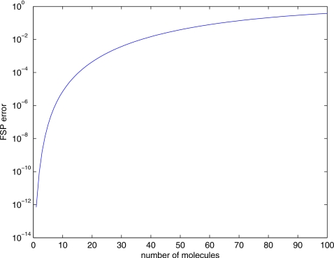
Next we perform an analysis of the adaptive step splitting error control. Consider the case where we want to calculate a final state of a subproblem containing 100 molecules of a chemical species after τD=0.1 using a local error tolerance of 10−5. If all 100 molecules are moved simultaneously, then the resulting single step FSP error will be 0.38 and our truncated state space contains 62% of the probability density. Utilizing the fact that the FSP error has a nonlinear relationship with the number of molecules moved (Fig. 1 shows the error as a function of the number of molecules moved in one time step), we can split the molecules into smaller groups where the sum of the error of diffusing the smaller groups is less than the original error. We recursively split a group of molecules in half if the error to move it in one step is greater than the error tolerance (adjusted for the recursion level). For 100 molecules, we first split them into two groups of 50 (error of 3.86×10⁻²), then four groups of 25 (error of 1.46×10⁻³), and so on. In total, we will move 12 groups of 6 molecules each with error of 2.4×10⁻⁷<10−5∕24=6.3×10⁻⁷ (four levels of recursion), four groups of 4 molecules each with error of 1.4×10⁻⁸<10−5∕25=3.1×10⁻⁷, and four groups of 3 molecules each with error of 1.6×10⁻⁹<10−5∕25=3.1×10⁻⁷ (both with five levels of recursion). The total error is 3.0×10⁻⁶, which is the sum of the error in all of the recursion steps. Using this method, we are able to satisfy the error tolerance, while continuing to utilize the efficiency of the lookup tables.
Figure 1.
Projection error (ϵ) for varying number of molecules given τD=0.1 s, ℓ=0.62 μm, and D=0.001 μm2 s−1. Adaptive step splitting allows us to take advantage of the independence of diffusing molecules and the nonlinear relationship of projection error to the number of molecules diffused to reduce the total error of diffusion step over τD by splitting it into sub-subproblems of fewer molecules rather than by splitting the time step.
Detailed algorithm descriptions
State space exploration
The algorithm to determine the truncated state space is presented in detail in Algorithm 1. The input parameters are the number nk of particles in the originating voxel k, and the maximum number of diffusive transfers MAX that a particle can move away from the originating voxel in one diffusion time step. The state representing the initial condition is that all nk particles are in the originating voxel. The algorithm is presented for an anisotropic, 1D Cartesian mesh with periodic boundary conditions, and assumes that the number of voxels in any dimension is large relative to MAX.
| |
| Algorithm 1 State Space Exploration |
| INPUT:nk, MAX, Initial State |
| OUTPUT:TransitionMatrixn, StateListn |
| 1: initialize: NextTierQueue←Initial State, Queue←∅ |
| 2: initialize: StateList←Initial State, TransitionMatrix←∅ |
| 3: for Tier ∊ (2, MAX) do |
| 4: Queue←NextTierQueue |
| 5: NextTierQueue←∅ |
| 6: for all states s∊Queuedo |
| 7: for all non-empty voxels v∊sdo |
| 8: for all inter-voxel transitions d {with probabilities p(d)} originating from vdo |
| 9: find state t←s+d(v) |
| 10: ift∉StateListthen |
| 11: add t to StateList, add t to NextTierQueue |
| 12: end if |
| 13: TransitionMatrix(s,t)←p(d) |
| 14: end for |
| 15: end for |
| 16: end for |
| 17: end for |
| 18: Update Diagonal elements in TransitionMatrix |
| 19: Truncate TransitionMatrix so that it is of dimension |StateList| |
| 20: Create absorbing state in TransitionMatrix |
We then store the TransitionMatrixn and StateListn for later use. For all cases where the number of particles in the originating voxel n, such that n is greater than MAX, the structure of the TransitionMatrixn is constant, and the values in the matrix are linear functions of n. This matrix is obtained by performing the state space exploration algorithm with n as an unspecified parameter constrained to a value greater than MAX. For n<MAX it is still necessary to go through the state space exploration, because for these values the TransitionMatrixn will not conform to the general structure.
DFSP diffusion step
This is the algorithm for taking a single time step of length τD for a single voxel k containing nk particles. We assume that TransitionMatrixn and StateListn have already been calculated and stored, and that MAX and τD are constant. Model parameters for the diffusion coefficient D and voxel length ℓ are also used.
Algorithm 2 shows the details of this process. The output of this algorithm is a vector map where the positions correspond to voxel indices and the values correspond to the number of particles that have traveled to that voxel from the originating voxel nk via diffusion after an interval of length τD seconds.
| |
| Algorithm 2 DFSP diffusion step with splitting |
| INPUT:nk, τD, TransitionMatrixn, StateListn, ErrorTolerancen |
| OUTPUT: Output State |
| 1: initialize once: PDVLookupTable, nmax←∞, L←0 |
| 2: ifnk>=nmaxthen |
| 3: return Output State←DFSP_Diffusion(⌊nk∕2⌋,L+1) +DFSP_Diffusion(⌈nk∕2⌉,L+1) |
| 4: else |
| 5: ifPDVLookupTable contains nkthen |
| 6: PDV←PDVLookupTable[nk] |
| 7: else |
| 8: PDV←exp(TransitionMatrixnk×D∕ℓ2×τD)×[1,0,0,⋯,0]T |
| 9: ifPDV[end]>ErrorTolerance∕2Lthen |
| 10: nmax←nk |
| 11: return Output State←DFSP_Diffusion(⌊nk∕2⌋) +DFSP_Diffusion(⌈nk∕2⌉) |
| 12: end if |
| 13: PDVLookupTable[nk]←PDV |
| 14: end if |
| 15: Generate a random number X∊U(0,1) |
| 16: Find the smallest integer μ such that |
| 17: return Output State←StateListnk[μ] |
| 18: end if |
Reactions
In our computational framework for reaction-diffusion problems, we use a fractional step method, which simulates the diffusive transfers by DFSP and the reaction events by SSA. We begin at t0 and calculate the first reaction event. We simulate reactions until the time to the next reaction would advance the simulation beyond t0+τD, at which point we forego the last reaction and perform a diffusion step using DFSP. After the diffusion step, the simulation is at time t0+τD. This process is repeated until the simulation is complete.
This process is detailed in Algorithm 3. Inputs to this algorithm are τD, the stoichiometric matrix ν, and the initial state of the system. The calls to DFSP_Diffusion use a StateList and TransitionMatrix that correspond to the geometry and jump propensities of the problem as well as a specified ErrorTolerance.
| |
| Algorithm 3 RDME simulation algorithm using DFSP for diffusion and SSA for reactions |
| 1: initialize system state: X, t=0 |
| 2: Calculate the propensity functions ajk(X) and {where M is the number of reactions and K is the number of voxels} |
| 3: Generate two random numbers r1,r2∊U(0,1) |
| 4: |
| 5: tnext_diff←t+τD |
| 6: whilet<tfinaldo |
| 7: iftnext_rxn<tnext_diffthen |
| 8: Find μr, μx smallest integers to satisfy |
| 9: Update Xμx(tnext_rxn)=Xμx(t)+νμr |
| 10: Generate two random numbers r1,r2∊U(0,1) |
| 11: t←tnext_rxn |
| 12: else |
| 13: Xnext←∅ |
| 14: fork∊(1…K) do |
| 15: fori∊(1…N) do |
| 16: Xnext←Xnext+DFSP_Diffusion(Xk,i) {diffusion of species i in voxel k} |
| 17: end for |
| 18: end for |
| 19: X←Xnext |
| 20: t←tnext_diff |
| 21: tnext_diff←t+τD |
| 22: end if |
| 23: Update propensity functions ajk(X) and |
| 24: |
| 25: end while |
EXAMPLES AND ANALYSIS
We examine two models to explore the validity, accuracy, and speed of DFSP. The first is a model of pure diffusion. The second is a biologically inspired reaction-diffusion spatial stochastic model.
Diffusion example
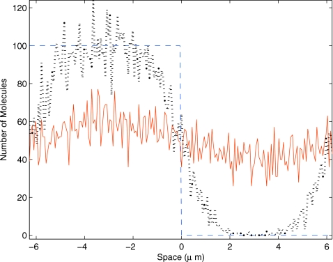
The first example is composed of a single chemical species diffusing in one dimension. The domain is periodic (Ω=12.4 μm) and we discretized it into 200 voxels with length of ℓ=0.062 μm. This domain is equivalent to a circle with a radius of 2 μm, so we will plot the results on the range of [−2π,2π). The initial condition is a step function such that each voxel in the range of [−2π,0) has 100 molecules and the remaining voxels are empty. The chemical species move with a diffusion coefficient of 0.001 μm2 s−1. Numerical experiments show that the relaxation time of this system is approximately 7000 s (data not shown). In this example, we use the adaptive step splitting with MAX=5. Figure 2 shows the initial condition (dashed blue), a transient state (dotted black), and a final state (solid blue) for a single sample trajectory of this model.
Figure 2.
Solution to a pure diffusion problem with a step function as the initial condition. Plotted is the state of the system at t=0 s (dashed blue), 500 s (dotted black), and 7000 s (solid red) for a stochastic trajectory. The domain is a circle with a radius of 2 μm, subdivided equally into 200 voxels.
Validation
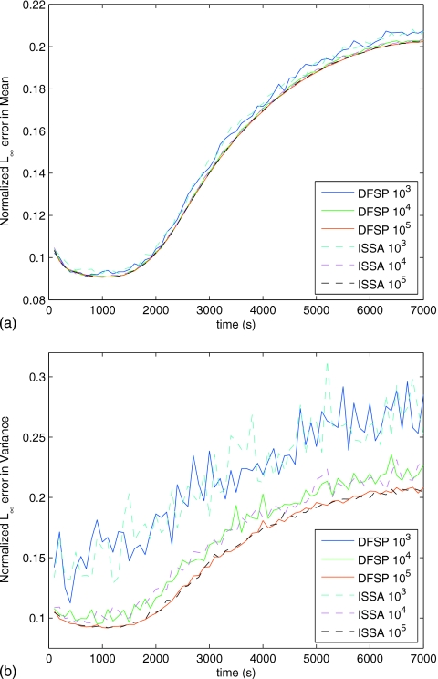
To test the validity of solving the diffusion example with ISSA or DFSP, we solve for the moments analytically (see Appendix A for derivation). Figure 3 shows the error in the mean and variance as a function of time for three different sized ensembles of ISSA and DFSP trajectories. The error is calculated using the L∞ norm (across space) of the difference between the ensemble moments and the analytically derived moments, divided by the norm of the analytical moment,
| (9) |
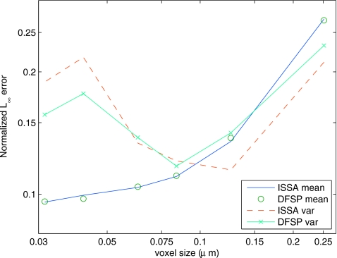
As the ensemble size increases, the error in both the mean and the variance decreases at the same rate for ISSA as DFSP. Figure 4 shows the error in the mean and variance as a function of the voxel size. As the voxel size decreases, the error decreases. This shows convergence of RDME solution methods to the analytical solution to the stochastic diffusion equation. Since the ISSA is an exact simulation method to the RDME while DFSP is an approximate method, this analysis shows that DFSP is just as valid as the ISSA for these parameter values.
Figure 3.
Plot of the normalized L∞ error (maximum deviation from analytical solution) vs time in the mean (a) and variance (b) for varying ensemble sizes for both DFSP (τD=0.1 s) and ISSA (voxel size of 0.06 μm) for an ensemble size of 103 trajectories. The error increases with time (as expected for a discretized solution) at the same rate for both DFSP and ISSA. Additionally, the error decreases (to the discretization error limit) with increasing ensemble size at the same rate for DFSP and ISSA.
Figure 4.
Plot of the normalized L∞ error vs voxel size (both on a log scale) calculated at t=100 s (a transient state) for an ensemble size of 103 trajectories. As voxel size decreases, the error in the mean decreases at the same rate for both DFSP and ISSA. The error in the variance shows a similar trend; however, it also shows increased error for small voxel sizes. This is mostly likely sampling error due to a constant system population distributed into an increasing number of voxels.
To assess the accuracy of DFSP, we treat an ensemble of ISSA simulations as the baseline distribution because the ISSA is a true realization of the RDME and its ensemble converges to the exact solution of the RDME. The Kolmogorov distance31 is a standard measurement of the difference between two cumulative distribution functions (CDFs), it is defined as the largest deviation between two CDFs. We choose this measure because it compares all the moments of two distributions and is thus a stronger tool for analysis than methods that use individual moments. We will plot the average Kolmogorov distance across space (Kmean) sampled at each point in time. This is given by
| (10) |
where N is the number of voxels. The CDFa(x,t) is calculated from an ensemble of trajectories generated by algorithm a (e.g., ISSA or DFSP) sampled at spatial location x at time t. We compare the Kmean of two independent ISSA ensembles (this is known as the self-distance) at each sampled point in time with the Kmean of an ISSA ensemble and a DFSP ensemble. If the two Kmean values are similar, then DFSP is statistically indistinguishable from ISSA for this ensemble size.
Figure 5 shows Kmean values across time for the ISSA self-distance and ISSA versus DFSP. We show results for ISSA versus DFSP for two sets of simulation parameters: the first uses τD=0.1 s, ErrorTolerance=10−5 and the second uses τD=1.9 s, ErrorTolerance=10−3. These results are for an ensemble size of 105 trajectories. We note that for an ensemble size of ≤104, DFSP is indistinguishable from ISSA (data not shown). These results show that for a sufficiently small values of τD and ErrorTolerance DFSP is a good approximation for ISSA. For the results with τD=1.9 s, the adaptive step splitting fails to meet the error tolerance; therefore, as the ensemble size grows the error accrued by DFSP is no longer negligible. Thus, it is clear that for increasing values of τD and ErrorTolerance the error in the simulation grows. We will show that it is possible to utilize this feature of DFSP to trade accuracy for computational performance.
Figure 5.
The distribution distance for the diffusion example, the Kmean at every 100 s for 7000 s for ISSA-vs-ISSA (green line with dots), ISSA-vs-DFSP with τD=0.1 s (dashed red line) and τD=1.9 s (blue line). In this plot the ensemble size is 105, at which point the DFSP solution becomes distinguishable from the ISSA solution for larger time steps. For ensemble sizes of ≤104, the DFSP solution is indistinguishable from the ISSA solution for both step sizes (results not shown).
Error analysis
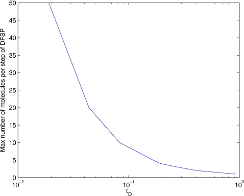
To study the error properties of DFSP, we must first find the limits of our adaptive step splitting error control method. The contribution from diffusion to the total error should be constant for all values of τD as long as we are able to move at least 1 molecule per DFSP diffusion step without violating our error tolerance. Figure 6 shows a plot of the maximum possible number of molecules moved per diffusion step of DFSP for various values of τD and a fixed error tolerance of 10−5. To find the maximum number of molecules we can move for a given τD, we compute DFSP matrix exponentials for increasing molecule counts. The maximum number that can be moved is 1 less than the number at which the estimate error first exceeds the tolerance. From this study, we determined that the maximum value of τD is 0.925 s.
Figure 6.
Maximum number of molecules moved in a single diffusion step of DFSP vs τD for an error tolerance of 10−5. Values of τD>0.925 s will try to move less than 1 molecule and thereby violate the error tolerance.
To measure the error in the simulated ensembles, we integrate the deviation between the K-distance of DFSP and ISSA and the self-distance of ISSA over space and time, normalized by the size of the domain,
| (11) |
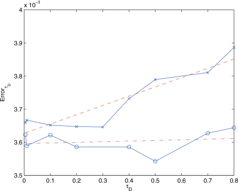
where ISSA(x,t) is the K-distance over space and time between two ensembles of 10 000 runs of the ISSA, and DFSPτD(x,t) is the K-distance over space and time between 10 000 runs of the DFSP algorithms (with diffusion step τD) and 10 000 runs of the ISSA algorithm. We examine this error metric for varying values of τD with a fixed error tolerance of 10−5. Figures 7 shows the error as a function of τD for the diffusion example as well as the G-protein example (discussed in Sec. 4B). This shows that for this range of values of τD, the error in the diffusion example is constant and a function only of the ErrorTolerance parameter.
Figure 7.
ErrorτD vs τD for the diffusion example (line with circles) and G-protein cycle example (line with x) and linear fits (dotted-dashed line and dashed line, respectively). For the diffusion example the error is constant and only a function of the error tolerance, this is because there is no contribution to the error from the reaction operator. For the G-protein cycle example the error increases linearly with τD and converges to the diffusion error as τD goes to zero. This is because the error in the reaction operator is linear with the time step (τD); as the time step goes to zero the reaction error goes to zero.
G-protein cycle example
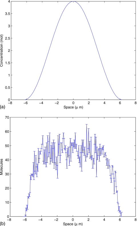
The second example is the pheromone induced G-protein cycle in Saccharomyces cerevisiae. We have converted the PDE model from Ref. 32 into a stochastic model and, for brevity, reduced it to ligand, receptor, and G-protein species. The ligand level is constant in time but it varies spatially (a cosine function) with parameters determined experimentally. The ligand binds stochastically with an initially isotropic field of receptor proteins. The bound receptor activates the G-protein, causing the Gα and Gβγ subunits to separate. Gα acts as an autophosphotase and upon dephosphorylation, rebinds with Gβγ to complete the cycle. The spatial domain is identical to the previous model and the simulation time is set to 100 s, as deterministic simulation shows that steady state is achieved by that time (data not shown). Gβγ is the component farthest downstream from the ligand input and acts as signal to the downstream Cdc42 cycle and will therefore be the output for this model. Figure 8 shows the constant ligand gradient (left) and the spatial distribution of Gβγ over 1000 runs (right, mean and standard deviation). See Appendix B for complete description of the reactions.
Figure 8.
Spatial concentration of ligand (a) and mean and variance of Gβγ molecules count (b) at t=100 s for a trajectory of the G-protein cycle example. The ligand gradient is the input to this model and is constant in time. Gβγ is the output and is time varying.
Validation
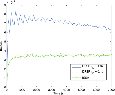
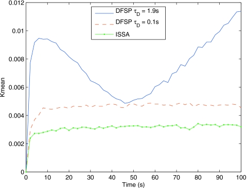
For the G-protein example, Fig. 9 shows the Kmean for ISSA versus DFSP (using τD=0.1 s, ErrorTolerance=10−5) for an ensemble size of 105 trajectories. Note that for an ensemble size of ≤103 trajectories, DFSP is indistinguishable from ISSA. For these simulation parameters, the difference between ISSA and DFSP values of Kmean is constant over time, and DFSP Kmean is consistent across the time span of the simulation. This indicates that the simulation is stable, but there is an error in the results that shows up as a difference between the DFSP and ISSA curves. We will discuss the source of this error and provide an analysis in the following section. We also show results for τD increased to the CFL limit,33 which is ∼1.9 s, and ErrorTolerance to 10−3 in an attempt to determine the limits of DFSP’s ability to handle full reaction-diffusion models. For these parameters the specified ErrorTolerance cannot be met, though the adaptive splitting moves a single molecule per step. The difference between this curve and the ISSA curve is significantly more, and is oscillatory in time. This indicates that the simulation results are inconsistent.
Figure 9.
The distribution distance for the G-protein cycle example, the Kmean from Eq. 10 at every 100 s for 7000 s for ISSA-vs-ISSA (green line with dots), ISSA-vs-DFSP with τD=0.1 s (dashed red line) and τD=1.9 s (blue line). In this plot the ensemble size is 105, at which point the DFSP solution becomes distinguishable from the ISSA solution for larger time steps. For ensemble sizes ≤103, the DFSP solution is indistinguishable from the ISSA solution for both step sizes (results not shown).
Error analysis
Over a given time step of length τD we first apply the reaction operator (SSA in this case) to the system, then the diffusion operator (using FSP) is applied to the resulting state of the system. Since these operators are decoupled, an additional splitting error is incurred by the method when reaction is included. Molecules that react in the timestep are not diffused, and molecules produced by a reaction in the timestep are diffused for the full length of the time step.
DFSP applied to the RDME is an operator split method, which is a first order Strang-splitting scheme,34 and as such, it is expected that the error should increase approximately linearly with τD. Figure 7 shows the error as a function of τD. We see that the error in the G-protein example is increasing approximately linearly with respect to τD and collapses to the error in the diffusion only system as τD goes to zero, confirming our expectation.
Performance
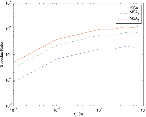
Figure 10 shows the speedup of DFSP over ISSA and MSA for the G-protein example. The performance increase for DFSP over ISSA and MSA is due in part to the difference in the number of times the reaction propensities must be updated as a result of diffusion events. For one realization, the expected number of diffusion events in an ISSA simulation is 1.2×10⁶. Thus, the reaction propensities must be updated approximately 2.4×10⁶ times (source and destination voxels for each diffusion event). By numerical experimentation, the average number of reaction events for any of the methods is ≥170 000. The time to the next diffusion event for MSA is given as the minimum of the time to the next reaction step and a predetermined time step; therefore, there must be at least as many diffusion events in a MSA simulation (regardless of stencil) as reaction events. For MSA, diffusion is done in all voxels, therefore updates need to be done in every voxel at each time step. Therefore, the expected number of reaction propensity updates in MSA due to diffusion steps is ≥3.4×10⁷. For DFSP with τD=0.1 s, 1000 diffusion steps are taken, and the reaction propensities are updated in every voxel on each DFSP step, resulting in 2×10⁵ reaction updates. Therefore, it is reasonable to expect that for this problem DFSP will be ∼102 times faster than MSA and ∼10 times faster than ISSA for τD=0.1 for this problem. Figure 10 validates this claim.
Figure 10.
Speedup of DFSP over ISSA and both MSA stencils (subscript 1 denotes the case where net diffusion is solved for adjacent voxels, and 2 the case where net diffusion is solved for the two nearest neighbors on either side) for varying values of τD for the G-protein cycle example. DFSP presents significant performance increases over ISSA and both MSA stencils for reaction-diffusion simulation. The speedup is due in part to the number of times the reaction propensity function needs to be updated due to diffusive transfers. DFSP updates less often than ISSA or MSA. As τD increases, the number of updates decreases and performance increases.
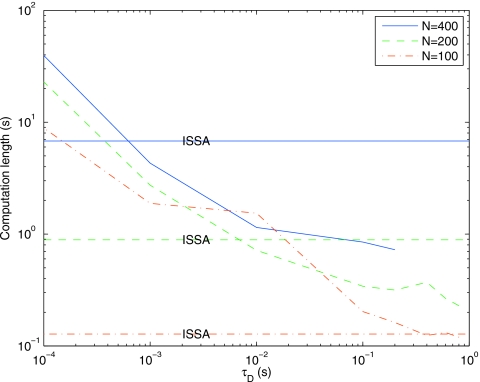
Next we examine the effect of different spatial discretization schemes on the performance. Figure 11 shows the computation time as a function of τD for three levels of mesh refinement, and the computation time for ISSA at each level for comparison. The computation time for DFSP does not vary as greatly as ISSA for different mesh sizes. In solving for the diffusion step of the algorithm, DFSP iterates over the voxels in the system and thus should scale linearly with the number of voxel. For comparison, in ISSA the number of diffusion jumps scales as 2∕ℓ2. Further calculations show that as we double the number of voxels the runtime for DFSP doubles, while for ISSA it increases by a factor of 8. This verifies our expectations.
Figure 11.
Computation time for DFSP with varying values of τD and varying numbers of voxels in the system with error tolerance of 10−5 for the diffusion example. ISSA computation times for each of the system sizes is provided for comparison.
For N=100, ISSA outperforms DFSP for the range of τD values shown. However, for this discretization level τD can be as large as 3.6 s, resulting in speedups proportional to the N=200 and N=400 mesh sizes. For reaction-diffusion systems, the fractional step decoupling error is proportional to τD. Thus, for coarse meshes where a large τD is possible, global accuracy constraints may force a parameter selection such that ISSA performs better than DFSP.
CONCLUSIONS
DFSP is a powerful new algorithm that yields impressive performance improvements over ISSA. DFSP provides a means to quantify and control the error, allowing a precise trade-off between accuracy and performance. Additionally, unlike many hybrid algorithms, DFSP conserves mass.
As multicore and graphics processing unit computing becomes even more prevalent, the importance of algorithms that are able to take advantage of these new technologies will increase. DFSP avoids many of the serial limitations imposed on spatial stochastic simulation. We are currently exploring enhancements that utilize these features. Another advantage of DFSP is that it extends simply to higher dimensional systems. This will be demonstrated in our future work.
The speedup offered by DFSP enables the simulation on a workstation of ensemble sizes that were previously feasible only on high performance clusters. It extends the scope of problems that are computable on high performance clusters. To produce our validation data for the G-protein cycle model we needed an ensemble of 100 000 runs for statistical accuracy. The DFSP algorithm generated this data set in 6.2 h (for τD=0.1 s and error tolerance of 10−5) and 3.8 h (for τD=1.9 s and error tolerance of 10−3) on a commodity desktop workstation with a quad-core processor (computing four trajectories simultaneously). The ISSA data sets were generated on a high performance computer cluster, so direct comparison is not possible. However, we estimate that each of the ISSA data sets would take approximately 472 processor hours, or 118 real hours (approximately 5 days) to calculate on the desktop workstation.
ACKNOWLEDGMENTS
We would like to thank Andreas Hellander and Dan Gillespie for their helpful comments.
The authors acknowledge research funding from the National Science Foundation through Grant Nos. ECCS-0835847, ECCS-0802008, and IGERT DGE-21715, U.S. Department of Energy under award DE-FG02-04ER25621, National Institutes of Health, Grant Nos. R01EB7511 and R01GM049831, and Institute for Collaborative Biotechnologies through Grant No. DAAD19-03-D-0004 from the U.S. Army Research Office.
APPENDIX A: ANALYTICAL SOLUTION TO THE DIFFUSION EXAMPLE
On a 1D infinite domain, if a single molecule is homogeneously distributed in the interval [a,b), then its probability distribution function p(x,t) is a step function
| (A1) |
We can evolve the probability distribution forward in time by solving the diffusion equation
| (A2) |
using Eq. A1 as the initial condition. The solution to the diffusion equation on a 1D infinite domain is the convolution of the initial condition with a Gaussian kernel,
| (A3) |
Since we seek to compare against numerical solutions solved on a discretized domain, we can use Eq. A3 to find the probability that a single molecule homogeneously distributed in the interval [a,b) (starting voxel) at t=0 will be in the interval [x1,x2) (ending voxel) at time t,
| (A4) |
For the solution on the domain [−2π,2π) with periodic boundary conditions, we can use mirroring. Mirroring is a method of translating a periodic domain into an infinite domain by repeating the initial condition function periodically from (−∞,∞). The problem is then solved by integrating across the infinite domain for solutions at points in the original domain,
| (A5) |
For finite precision of our answer, we need take only a finite number of terms
| (A6) |
where 2J+1 is a sufficient number of terms for the required precision of our solution.
For the diffusion example (see Fig. 2), the step function initial conditions is equivalent to homogeneously distributing 100 molecules in each of the 100 voxels in the interval [−2π,0] (for ℓ=0.06 μm). If a molecule starts in the kth voxel, and we want to know the probability that it will be within a given voxel containing the interval [x,x+ℓ) at time t, we can use Eq. A6 with the following inputs:
| (A7) |
To compare to our numerical solutions, we need to find the moments of the population of molecules in a given voxel at a given time. The generic binomial distribution is a sum of many independent Bernoulli trials and the mean and the variance of such a distribution are equal to the sums of the means and variances of each individual trial. A molecule being located within a given voxel at time t is a Bernoulli trial with probability given by Eq. A6 because it is either within the voxel or it is not. Thus, the population u(x,t) of a voxel containing the interval [x,x+ℓ) at any time t is binomially distributed, and the analytical solution for the mean and variance of the population is given by
| (A8) |
| (A9) |
where nk is the initial population of the voxel containing the interval [x,x+ℓ).
We can use Eqs. A8, A9 to compare the mean and variance obtained from an ensemble of runs from ISSA and DFSP.
APPENDIX B: G-PROTEIN CYCLE EXAMPLE
These are the equations that describe the reactions of the G-protein cycle example.
Equations
| (B1) |
| (B2) |
| (B3) |
| (B4) |
| (B5) |
| (B6) |
| (B7) |
| (B8) |
Rate constants
Total populations and initial conditions
References
- McAdams H. and Arkin A., Proc. Natl. Acad. Sci. U.S.A. 94, 814 (1997). 10.1073/pnas.94.3.814 [DOI] [PMC free article] [PubMed] [Google Scholar]
- Elowitz M., Levine A., Siggia E., and Swain P., Science 297, 1183 (2002). 10.1126/science.1070919 [DOI] [PubMed] [Google Scholar]
- Gillespie D., Annu. Rev. Phys. Chem. 58, 35 (2007). 10.1146/annurev.physchem.58.032806.104637 [DOI] [PubMed] [Google Scholar]
- Howard M. and Rutenberg A. D., Phys. Rev. Lett. 90, 128102 (2003). 10.1103/PhysRevLett.90.128102 [DOI] [PubMed] [Google Scholar]
- Fange D. and Elf J., PLOS Comput. Biol. 2, e80 (2006). 10.1371/journal.pcbi.0020080 [DOI] [PMC free article] [PubMed] [Google Scholar]
- Doubrovinski K. and Howard M., Proc. Natl. Acad. Sci. U.S.A. 102, 9808 (2005). 10.1073/pnas.0500529102 [DOI] [PMC free article] [PubMed] [Google Scholar]
- Elf J. and Ehrenberg M., IEE Proceedings Systems Biology, 2004. (unpublished), Vol. 1, p. 230. [DOI] [PubMed]
- Munsky B. and Khammash M., J. Chem. Phys. 124, 044104 (2006). 10.1063/1.2145882 [DOI] [PubMed] [Google Scholar]
- Gardiner C. W., McNeil K. J., Walls D. F., and Matheson I. S., J. Stat. Phys. 14, 307 (1976). 10.1007/BF01030197 [DOI] [Google Scholar]
- Shnerb N., Louzoun Y., Bettelheim E., and Solomon S., Proc. Natl. Acad. Sci. U.S.A. 97, 10322 (2000). 10.1073/pnas.180263697 [DOI] [PMC free article] [PubMed] [Google Scholar]
- Isaacson S., SIAM J. Appl. Math. 70, 77 (2009). 10.1137/070705039 [DOI] [Google Scholar]
- Erban R. and Chapman S., Phys. Biol. 6, 046001 (2009). 10.1088/1478-3975/6/4/046001 [DOI] [PubMed] [Google Scholar]
- Gibson M. and Bruck J., J. Phys. Chem. A 104, 1876 (2000). 10.1021/jp993732q [DOI] [Google Scholar]
- Hattne J., Fange D., and Elf J., Bioinformatics 21, 2923 (2005). 10.1093/bioinformatics/bti431 [DOI] [PubMed] [Google Scholar]
- Marquez-Lago T. T. and Burrage K., J. Chem. Phys. 127, 104101 (2007). 10.1063/1.2771548 [DOI] [PubMed] [Google Scholar]
- Lampoudi S., Gillespie D., and Petzold L., J. Chem. Phys. 130, 094104 (2009). 10.1063/1.3074302 [DOI] [PMC free article] [PubMed] [Google Scholar]
- Zheng Z., Stephens R., Braatz R., Alkire R., and Petzold L., J. Comput. Phys. 227, 5184 (2008). 10.1016/j.jcp.2008.01.056 [DOI] [Google Scholar]
- Rodriguez J., Kaandorp J., Dobrzynski M., and Blom J., Bioinformatics 22, 1895 (2006). 10.1093/bioinformatics/btl271 [DOI] [PubMed] [Google Scholar]
- Ferm L., Hellander A., and Lötstedt P., Technial Report No. 2009-010 (Department of Information Technology, Uppsala University, 2009).
- Engblom S., Ferm L., Hellander A., and Lötstedt P., SIAM J. Sci. Comput. (USA) 31, 1774 (2009). 10.1137/080721388 [DOI] [PMC free article] [PubMed] [Google Scholar]
- Gillespie D., Physica A 188, 404 (1992). 10.1016/0378-4371(92)90283-V [DOI] [Google Scholar]
- Gillespie D., J. Phys. Chem. 81, 2340 (1977). 10.1021/j100540a008 [DOI] [Google Scholar]
- Cao Y., Li H., and Petzold L., J. Chem. Phys. 121, 4059 (2004). 10.1063/1.1778376 [DOI] [PubMed] [Google Scholar]
- Slepoy A., Thompson A., and Plimpton S., J. Chem. Phys. 128, 205101 (2008). 10.1063/1.2919546 [DOI] [PubMed] [Google Scholar]
- Li H. and Petzold L., Int. J. High Perform. Comput. Appl. (2009). 10.1177/1094342009106066 [DOI]
- Gillespie D., J. Chem. Phys. 115, 1716 (2001). 10.1063/1.1378322 [DOI] [Google Scholar]
- Peleš S., Munsky B., and Khammash M., J. Chem. Phys. 125, 204104 (2006). 10.1063/1.2397685 [DOI] [PubMed] [Google Scholar]
- McNamara S., Burrage K., and Sidje R., Int. J. Comput. Sci. 2, 402 (2008). [Google Scholar]
- Munsky B. and Khammash M., J. Comput. Phys. 226, 818 (2007). 10.1016/j.jcp.2007.05.016 [DOI] [Google Scholar]
- Burrage K., Hegland M., MacNamara S., and Sidje R., in Proceedings of the 150th Markov Anniversary Meeting, edited by Langville A. and Stewart W. (Boson Books, Raleigh, NC, 2006), p. 2138.
- Kolmogorov A., IEEE Trans. Inf. Theory 14, 662 (1968). 10.1109/TIT.1968.1054210 [DOI] [Google Scholar]
- Chou C. -S., Nie Q., and Yi T. -M., PLoS ONE 3, e3103 (2008). 10.1371/journal.pone.0003103 [DOI] [PMC free article] [PubMed] [Google Scholar]
- Courant R., Friedrichs K., and Lewy H., Math. Ann. 100, 32 (1928). 10.1007/BF01448839 [DOI] [Google Scholar]
- Strang G., SIAM (Soc. Ind. Appl. Math.) J. Numer. Anal. 5, 506 (1968). 10.1137/0705041 [DOI] [Google Scholar]


