

Abstract
A phase-locked loop (PLL) model of the response of the postural control system to periodic platform motion is proposed. The PLL model is based on the hypothesis that quiet standing (QS) postural sway can be characterized as a weak sinusoidal oscillation corrupted with noise. Because the signal to noise ratio is quite low, the characteristics of the QS oscillator are not measured directly from the QS sway, instead they are inferred from the response of the oscillator to periodic motion of the platform. When a sinusoidal stimulus is applied, the QS oscillator changes speed as needed until its frequency matches that of the platform, thus achieving phase lock in a manner consistent with a PLL control mechanism. The PLL model is highly effective in representing the frequency, amplitude, and phase shift of the sinusoidal component of the phase-locked response over a range of platform frequencies and amplitudes. Qualitative analysis of the PLL control mechanism indicates that there is a finite range of frequencies over which phase lock is possible, and that the size of this capture range decreases with decreasing platform amplitude. The PLL model was tested experimentally using nine healthy subjects and the results reveal good agreement with a mean phase shift error of 13.7° and a mean amplitude error of 0.8 mm.
Index Terms: Mathematical model, phase-locked loop, postural control
I. Introduction
The ability of humans to stand upright and maintain balance in the presence of disturbances is achieved through the postural control system. Postural control consists of both postural steadiness associated with the ability to maintain balance during quiet standing, and postural stability that is associated with the response to applied external disturbances and volitional postural movements [1]. The postural control system makes use of information from the visual, vestibular, and somatosensory systems [2].
Balance is achieved when the subject’s center of gravity (COG) remains within the base of support. The COG is the vertical projection of the center of mass onto the base of support. It is a whole body characteristic that is difficult to directly measure, so typically the center of pressure (CoP) is used instead. The CoP is the location of the vertical ground reaction force on the surface upon which the subject stands. CoP movements are used to control the horizontal displacements of the center of mass. In general the CoP varies about the COG, but with higher amplitude and higher frequency content [3]. Using a single force plate, it is the net CoP from both feet that is measured [4]. Over an extended period of time of quiet stance, the average of the CoP must equal the average of the COG [5].
During quiet standing, humans sway to maintain balance; and this motion can be measured using the anterior–posterior (AP) and the medial–lateral (ML) components of the CoP. Different control mechanisms and different muscle groups are used to control AP and ML motion [3]. Most mathematical models of the postural control system are biomechanical and employ a 1-D or 2-D inverted pendulum structure [6]–[9]. Some look at the contributions of each leg separately and, therefore, include a pair of inverted pendulums [4], [5]. Others are more refined and include an articulated chain of links interconnected by joints to model the effects of the ankles, knees, hips, shoulders, elbows, and neck [5]. One control system strategy suggests that high ankle stiffness accounts for most, but not all, of postural steadiness [10]–[13]. Another approach employs continuous linear feedback including proportion plus derivative (PD) and proportional plus integral plus derivative (PID) control [14]–[16]. Both of these approaches achieve asymptotic stability with the residual sway movements being noise driven. Another control system representation has been proposed that relies on an intermittent controller that becomes activate when the sway motion moves outside of a small dead zone [7], [17]. Here the persistent sway patterns are not noise driven but result from the limited resolution of the controller.
Most of the control system model focus on the question of postural steadiness or the ability to maintain balance during quiet standing. This paper focuses on the development of a control system model that characterizes postural sway when human subjects are exposed to periodic disturbances whose frequencies and amplitudes vary [14], [18]. It is hypothesized that quiet standing motion can be represented mathematically as a noise-corrupted oscillation. A nonlinear phase-locked loop (PLL) structure is used to control both the frequency and the amplitude of the quiet standing oscillator when a periodic stimulus is applied [19]. If the stimulus amplitude is sufficiently large and the stimulus frequency is sufficiently close to the quiet standing frequency, the oscillator will achieve phase lock with a well-defined phase angle between the periodic disturbance and the steady-state response. Measurements of the amplitude and the phase of the steady-state response are used to identify parameters of a PLL model.
To test this notion, subjects stood on an air bearing platform that was made to undergo sinusoidal AP motion in order to generate a periodic disturbance to the postural control system. The measured response was the CoP of the subjects along the direction of platform motion. Nine healthy young adults were tested to collect the experimental data used to develop and test the model. The results show that a PLL structure is highly effective in describing the experimental behavior observed in this study.
II. Method
A. Subjects and Testing Procedures
To develop and test the proposed postural control system model, experimental sway measurements were taken for sinusoidal disturbances. The set of subjects consisted of nine healthy young adults ranging in age from 20 through 29 years. The number of males was seven and there were two females. The subjects were recruited from the community by advertising at Clarkson University. The recruiting, screening, testing, and informed consent procedures were reviewed and approved by the appropriate Institutional Review Board. The subjects that were recruited for this investigation all underwent visual, vestibular, auditory, musculoskeletal, and cognitive screening to maximize the likelihood that they had no undiagnosed conditions that may have affected their balance [20].
The experimental data were obtained using the SLIP-FALLS system, a sliding linear investigative platform for analyzing lower limb stability [21]. This is a computer-controlled air-bearing mobile platform instrumented with a force plate to precisely measure CoP. For the quiet standing portion of this study the platform was held motionless, and the subjects stood barefoot with their arms at their sides. Throughout the data collection, the backs of both heels were aligned in the frontal plane, with feet splayed out at natural stance. In the ML direction, subjects were asked to maintain their normal width stance. In order to minimize the effects of visual and audio cues, the subjects were blindfolded, and headphones were used to provide masking noise (70 dB SPL) and instructions. The use of the eyes-closed condition during 60 s of quiet stance did not appear to have any detrimental effects on the subjects.
Each subject was also exposed to four trials, each of duration 120 s, where the platform underwent sinusoidal motion in the AP direction. Two of the frequencies used were fixed at 0.5 and 0.75 Hz. The other two frequencies were determined using the two largest peaks in the power density spectrum of the quiet standing sway. For each frequency, the amplitude used was determined by first measuring a psychophysical threshold in which the subject is able to correctly perceive that the platform is moving 75% of the time. A modified single-interval-adjustment matrix (mSIAM) protocol based on 30 trials was used to adaptively compute the threshold amplitude [22]. The resulting sinusoidal amplitudes were quite small with a mean of 1.08 mm, and they varied from subject to subject.
III. A PLL Model
A. Quiet Standing Oscillator
Since humans sway in order to maintain balance, it seems reasonable to assume that there is some form of underlying oscillation involved. For control system models that are asymptotically stable such as ankle stiffness and PID feedback control, the oscillation is noise driven. Alternatively, an intermittent or burst controller has been proposed that achieves bounded stability with oscillations that are the result of a limited-resolution controller [7]. Another approach suggests that imperfect perception of the body in space (state estimation error) explains why humans sway slowly during quite stance [14], [23]. Our focus is on the response of the postural control system to periodic disturbances. Consequently, no attempt is made to develop a detailed biomechanical model of quiet standing sway itself. Instead, the following high-level representation of postural sway is employed that consists of a sinusoidal oscillation corrupted with additive noise
| (1) |
| (2) |
Here, y(t) is the AP CoP, while Aq, ωq, and φq are the amplitude, frequency, and phase, respectively, of an underlying quiet standing (QS) oscillator. The additive noise consists of white noise v(t) processed by a linear filter whose impulse response, hq(t), shapes the spectrum of the observed noise, d(t). The representation of y in (1) and (2) corresponds to the Wold decomposition of a stationary random process into the sum of a general linear process d(t) plus a predictable process, xq(t), [24]. In order to identify the parameters of the QS oscillator from samples of the AP CoP, it is useful to convert the system in (1) and (2) to a discrete-equivalent model. Suppose ωs is the sampling frequency, T= 2π/fs is the sampling interval, and k denotes discrete time. Then (1) and (2) can be written as follows where an nth order auto-regressive filter is used to shape the spectrum of the noise
| (3) |
| (4) |
1) Extracting a Sinusoid
Suppose the measured postural sway consists of the N samples y(k) for 0 ≤ k < N. When the platform is driven by a sinusoidal stimulus, it will be necessary to estimate the amplitude, frequency, and phase angle of the sinusoidal component of the steady-state response. In [25] a statistical approach was applied to visually-induced sway using sinusoidal optical flow at two frequencies. In this paper a normalized cross-correlation approach is used because it is effective in the presence of noise, and it provides an indication of the degree of entrainment. To estimate the sinusoidal component of the AP CoP, consider a cosine of frequency ω and unit amplitude
| (5) |
Let ρyx(j) denote the normalized cross correlation of y with x where j is the lag variable and −1 ≤ ρyx(j) ≤ 1 for 0 ≤ j < N. The peak normalized cross correlation of y with x can be regarded as a function of ω
| (6) |
The value of ω at which ρmax(ω) achieves a maximum is used to estimate the frequency
| (7) |
The peak normalized cross correlation, ρmax(ω), can have a number of local maxima. However, since the frequency interval is bounded, one can start by examining the value of ρmax(ωi) at the N discrete frequencies wi = iΔω for 0 < N where Δω = ωs/N is the precision of the DFT of y(k). Once a discrete frequency ω̂ that maximizes ρmax(ωi) is found, the search process then can be repeated over the smaller interval [ω̂ − Δω, ω̂ + Δω]. This step-wise refinement can be repeated as needed until the desired precision is reached. The optimal phase angle, φ̂, is obtained from the lag J at which the peak normalized cross correlation in (6) occurs
| (8) |
Given ω̂ and φ̂, the corresponding amplitude  is determined by minimizing the sum of the squares of the error e(k) = y(k) − A cos(kω̂T + φ̂). Let z(k) = cos(kω̂T + φ̂) and suppose y ∈ RN and z ∈ RN are column vectors. Then
| (9) |
This results in the following sinusoidal component of postural sway
| (10) |
The peak normalized cross correlation ρmax(ω̂) can be used to determine the relative strength of the sinusoidal component of the sway. For the idealized case y(k) = x̂(k), the peak is ρmax(ω̂) = 1. The relative strength of x̂(k) also can be expressed in terms of the signal to noise ratio using x̂(k) as the signal and d(k) = y(k) − x̂(k) as the noise. Plots of the CoP and platform for a 24-year-old healthy female are shown in Fig. 1. The heavy lines show the extracted sinusoids of the CoP (ρmax = 0.38)and platform ρmax = 0.99). The platform cross correlation is not quite 1.0 due to the start up transient which delays the sinusoidal platform motion by about two seconds. Here N = 12000 and fs = 100 Hz.
Fig. 1.

Extraction of the sinusoidal components of CoP and platform data for a 24-year-old healthy female. The numbers in parentheses are the peak cross correlations.
2) Noise Parameters
The technique outlined in (7)–(9) can be used to extract the sinusoidal component of the postural sway both with the platform moving and the platform still. However, when the platform is motionless, the extracted QS signal typically has a relatively weak peak cross correlation, ρmax(ω̂), indicating that the signal to noise ratio is poor. Since the quiet standing oscillation is often buried deep within the noise, the frequency of the quiet standing oscillator will instead be inferred from phase shift measurements when the postural sway is phased-locked to periodic motion of the platform. Once the quiet standing frequency ωq is obtained in this manner, the quiet standing phase φq and amplitude Aq can be computed using (8) and (9), respectively.
Given the sinusoidal component of the QS sway, the additive noise can be computed from (3). An auto-regressive filter of order n is used to shape the spectrum of the white noise v(k) to match that of d(k). The coefficient vector a ∈ Rn can be computed by solving the Yule-Walker equations [24] using the autocorrelation of d(k).
B. Phase-Locked Loop
When a sinusoidal stimulus is applied to the platform, the steady-state CoP typically becomes phase-locked with the periodic stimulus. Phase lock can be interpreted as the QS oscillator changing speed, as needed, until its frequency exactly matches that of the periodic stimulus. This interpretation suggests a phase-locked loop (PLL) feedback structure, as shown in Fig. 2 [19]. Here the nonlinear PLL consists of a phase detector in the form of a multiplier, a first-order low pass loop filter, and the QS oscillator with amplitude one and adjustable frequency ω.
Fig. 2.

PLL model of the QS oscillator driven by periodic motion of the platform.
1) Hold in Range
To analyze the steady-state operation of the PLL, suppose the platform moves in a sinusoidal manner with amplitude Ai and frequency ωi
| (11) |
Consider the case when the frequency of the QS oscillator exactly matches that of the platform
| (12) |
Using a trigonometric identity, the multiplier output xd(t)contains a sum frequency term and a difference frequency term
| (13) |
If τf > 1/(2ωi), then the second harmonic will be attenuated by the loop filter, and only the dc term will appear in the filter output
| (14) |
For phase lock to occur, it is necessary that ωq + xf = ωi. Setting ωi − ωq equal to xf in (14) and solving for θ yields the QS oscillator phase shift during phase lock
| (15) |
From (15) it is clear that phase lock is possible only for input frequencies ωi and input amplitudes Ai that satisfy the following constraint:
| (16) |
This is the hold-in range of the PLL where phase lock is possible, but not guaranteed. The subset of the hold-in range over which phase lock occurs is the capture range of the PLL [19].
The first-order loop filter is not an ideal low pass filter. Consequently, during phase lock the oscillator frequency ω(t) will be periodic with period 2π/ωi, but it will have a mean value of E[ω(t)] = ωi. The higher-order low pass filter HL(s) in Fig. 2 provides a smoothed estimate of the input frequency ωi. For example, a fourth-order low pass Butterworth filter with a cutoff frequency of Fc = 0.1 Hz can be used.
2) PLL Parameters
Suppose that M measurements of the phase shift θi are available corresponding to sinusoidal inputs with amplitude Ai and frequency ωi for 1 ≤ i ≤ M. The parameters of the PLL that must be determined are the loop filter time constant τf, and the loop filter gain Af. The loop filter time constant should be set to produce a cutoff frequency ωc = 1/τf that removes the second harmonic at 2ωi. For example, the following cutoff provides reasonable attenuation
| (17) |
The loop filter gain Af must be selected to ensure that the ωi and Ai fall well within the hold-in range for 1 ≤ i ≤ M. For example, suppose θ in (15) is set to θM = π/4. Setting α = |ωi − ωq|/Ai to its maximum value and solving for Af yields the following loop filter gain
| (18) |
| (19) |
Since Af can become very large as Ai approaches zero, for practical reasons Ai is replaced in (18) by max{Ai, 0.2} to limit the loop filter gain. For the nine subjects, two of the input frequencies were common, Fi = 0.5 Hz and Fi = 0.75 Hz. Plots of the variable F(t) = xF(t)/(2π)for the two common frequencies are shown in Fig. 3. It is clear that the PLL has locked onto the platform frequency in each case.
Fig. 3.

The smoothed PLL frequency, F = xF/(2π), for nine subjects for platform frequencies of 0.5 Hz and 0.75 Hz.
C. Amplitude Control
A PLL based on the QS oscillator can be used to represented the phase shift between the steady-state CoP and sinusoidal platform motion. However, the amplitude of the PLL oscillator remains fixed at one, independent of input amplitude Ai and input frequency ωi. During phase lock, xF ≈ ωi. To measure the input amplitude, Ai, a basic envelope detector system can be used that consists of a nonlinear element F(u) = (π/2)|u| followed by a low pass filter
| (20) |
When u(t) is sinusoidal as in (11), the periodic signal xa(t) = (π/2)|u(t)| contains a dc term, Ai, plus second and higher order harmonics. The function of the low pass filter HL(s) is to remove the harmonics. This is the same role played by the low pass loop filter in Fig. 2 and results in the envelope detector output, xA(t) ≈ Ai.
D. Propagation Delay
The overall PLL model of sway motion includes a PLL block and an envelope detector block configured as shown in Fig. 4. The system in Fig. 4 also includes a propagation delay τd, and an amplitude gain function G.
Fig. 4.

Overall PLL model of CoP during quiet standing and periodic motion of the platform.
The delay τd represents the time required for signal propagation associated with neural transmission, sensory processing, and muscle activation. The propagation delay contributes φd = − τdω to the overall phase shift between u(t) and xP(t). Thus the total phase shift can be obtained by adding − τdωi to the PLL phase shift θ(ωi, Ai) in (15). To determine a suitable value for the delay τd, recall that θi represents the measured phase shift. The propagation delay is chosen to account for as much of the observed phase shift as possible by selecting τd to minimize the sum of the squares of the error, ei = θi + τdωi for 1 ≤ i ≤ M. This yields the following least-squares propagation delay where w ∈ RM and θ ∈ RM are column vectors
| (21) |
The residual phase shift, Δθ(ω) = θ + ωτd, represents the component of the phase shift associated with the PLL. Suppose a first-order polynomial Δθ(ω) ≈ p1ω+ p2 is fitted to the residual phase shift data Δθ(ωi) for 1 ≤ i ≤ M using a least-squares fit. The frequency at which the residual phase shift is zero is then ω = −p2/p1. From (15), the PLL contributes a phase shift of zero when ω =ωq. Consequently, the frequency of the QS oscillator is set as follows:
| (22) |
1) Amplitude Parameters
The remaining component in Fig. 4 is the amplitude gain function G. Note that the amplitude of the sinusoidal oscillation xq(t) appearing in output y(t) is a = G(xA, xF). For the amplitude gain function, the following first-order bilinear form is used:
| (23) |
Recall that xA ≈ Ai, and when the PLL is locked, xF ≈ ωi. During quiet standing, (xA, xF) = (0, ωq), and the QS oscillator amplitude is a = Aq. To determine values for the coefficient vector g ∈ R3, let Bi represent the measured amplitude of the QS oscillator when the platform is driven with a sinusoid of frequency ωi and amplitude Ai for 1 ≤ i ≤ M. Next define the M × 3 coefficient matrix D, and the M × 1 right-hand side vector b as follows:
| (24) |
| (25) |
For M >3, the linear algebraic system Dg = b is over determined, and the least-squares solution for the coefficient vector g is
| (26) |
IV. Results
A. Individual Models
The CoP data are available as sampled signals with a sampling rate of fs = 100 Hz. Consequently, the PLL sway model is converted to discrete-equivalent form using a backward Euler approximation for the loop filter, and a trapezoid rule integrator for the QS oscillator.
The experimental data used to identify and test the model consisted of 2M +1 discrete-time signals from each of the nine subjects. These included a vector Q ∈ RP/2 representing 60 s of quiet standing AP CoP sway where P =12000. The data also included a matrix U ∈ RP × M whose columns contained the platform samples for M = 4 sinusoidal trials, each of duration 120 s with each trial corresponded to a particular input frequency ωi and input amplitude Ai. The corresponding AP CoP was recorded in Y ∈ RP × M.
The parameter identification methods for the PLL model were applied to each of the subjects with the results summarized in Table I. The parameter Fq = ωq/(2π) is the quiet standing frequency, or center frequency of the PLL, expressed in hertz. The loop filter parameters, τf and Af, are determined by applying (17)–(19) using the range of platform frequencies, ωi, and amplitudes, Ai. The latter serve to define the domain over which the PLL model is defined. Similarly, the amplitude parameters, g ∈ R3, are determined using (24)–(26).
Table I.
Parameters of PLL Model. The Last Rows are the Mean, μ, and the Standard Deviation, σ. Here Eθ, and Eα are the Means of the Phase Shift Error, and Amplitude Error, Respectively
| Age year | τd s | Fq Hz | Aq mm | Tf s | Af | Lock % | Eθ deg | Ea mm |
|---|---|---|---|---|---|---|---|---|
| F24 | 0.25 | 0.55 | 0.1 | 0.22 | 6.2 | 100 | 17.5 | 1.1 |
| F28 | 0.19 | 0.56 | 0.9 | 0.20 | 5.1 | 100 | 14.0 | 0.1 |
| M20 | 0.33 | 0.77 | 2.2 | 0.16 | 13.6 | 50 | 13.7 | 2.2 |
| M20 | 0.30 | 0.83 | 1.7 | 0.16 | 12.9 | 100 | 9.3 | 0.2 |
| M24 | 0.39 | 0.89 | 3.4 | 0.16 | 23.7 | 50 | 20.8 | 2.1 |
| M24 | 0.20 | 0.59 | 0.3 | 0.26 | 10.0 | 100 | 15.3 | 0.4 |
| M24 | 0.18 | 0.62 | 0.6 | 0.19 | 2.9 | 100 | 6.2 | 0.6 |
| M27 | 0.30 | 0.73 | 0.6 | 0.24 | 35.3 | 100 | 10.8 | 0.1 |
| M29 | 0.23 | 0.69 | 0.1 | 0.20 | 9.5 | 100 | 15.5 | 0.3 |
| μ | 0.26 | 0.69 | 1.1 | 0.20 | 13.2 | 89 | 13.7 | 0.8 |
| σ | 0.07 | 0.12 | 1.1 | 0.04 | 10.3 | 22 | 4.4 | 0.8 |
To measure phase shift, first (7)–(9) were used to find the frequency ωi, phase angle φ;i, and amplitude Ai of the platform for the ith trial. Similarly, (7)–(9) were used to determine the frequency Ωi, phase angle ψi, and amplitude Bi of the CoP. The two signals were regarded as phase locked when |ωi − Ωi| < ωs/(2P) and ρmax(Ωq) > 0.2. The threshold, Δω = ωs/(2P), corresponds to the frequency precision available from a DFT of the data. Using this criterion, the CoP sway was phase locked to the platform in 89% of the trials. It is not surprising that two of the subjects achieved phase lock only 50% of time because a low platform amplitude, corresponding to a psychophysical threshold, was used. Once the phase lock was determined, (8) and (9) were applied with ω = ωi to determine the phase angle ψi and amplitude of Bi of the CoP. This was done because the phase shift θi = ψi − φi only has meaning when the frequencies match.
Let θpi = ψpi − φi denote the corresponding phase shift associated with the PLL model for 1 ≤ i ≤ M. The following mean phase shift error can be used to measure the effectiveness of the PLL model in characterizing the steady state postural sway during periodic motion of the platform
| (27) |
The mean of Eθ for the group of subjects was μ = 13.7° and the standard deviation was σ = 4.4°. The CoP and PLL phase shifts for one female subject and one male subject are shown in Fig. 5. For these two cases from Table I, the mean phase shift errors were 14.0° and 15.3°, respectively.
Fig. 5.

Phase shift of the sinusoidal component of AP CoP for (a) a healthy 28-year-old female subject and (b) a healthy 24-year-old male subject.
Next recall that Bi denotes the measured amplitude of the sinusoidal component of the sway for the ith trial. If Bpi denotes the corresponding amplitude associated with the PLL model, then the following mean amplitude error can be used to measure the effectiveness of the PLL model in characterizing the steady state postural sway during periodic motion of the platform:
| (28) |
The mean of Ea for the group of subjects was μ = 0.8 mm and the standard deviation was σ = 0.8 mm. The CoP and PLL amplitudes for the same pair of female and male subjects are shown in Fig. 6. For these two cases, the mean amplitude errors were 0.1 mm and 0.4 mm, respectively. At the lower frequencies, the PLL oscillator output can exhibit harmonic distortion due to the ripple in ω(t). Consequently, the peak value of xq(t) was used to compute the amplitude Bpi in (28).
Fig. 6.

Amplitude of the sinusoidal component of AP CoP for (a) a healthy 28-year-old female subject and (b) a healthy 24-year-old male subject.
B. Composite Model
Although the platform frequencies and amplitudes vary from subject to subject, all of the experimental phase shift data can be plotted on a single graph if a normalized version of the platform frequency is used. Recalling (15), the following normalized frequency variable takes on values between and −1 over the hold in range of the PLL:
| (29) |
Using λ as the independent variable, plots of the total phase shift θ are shown in Fig. 7. To facilitate a comparison between the CoP data and PLL model, straight line least-squares fits are also shown. Although there is clearly variation in the phase shift data when all of the subjects are included, it is apparent from the trend lines that there is good overall agreement between the data and the PLL model.
Fig. 7.
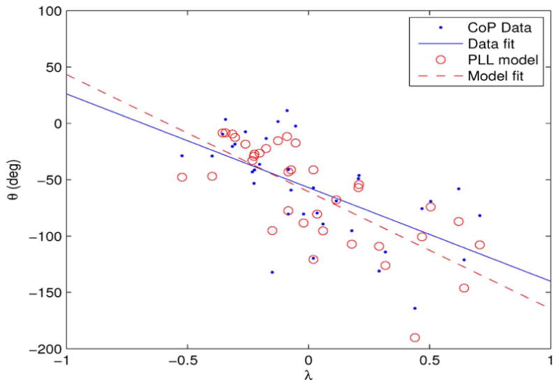
CoP and PLL phase shifts versus normalized frequency. The r2 value for the CoP linear regression is 0.36 and for the PLL linear regression is 0.53.
The other characteristic of the sinusoidal component of the sway during phase lock is the amplitude of the sway. For linear systems, the amplitude of the output is proportional to the amplitude of the input with the gain, γ = B/A, being dependent on the input frequency. A plot of amplitude gain is shown in Fig. 8. Again to facilitate a comparison between the CoP data and the PLL model, straight line least squares fits are included. It is evident that there is very good agreement which is not surprising since the amplitude gain function G was determined by using three coefficients to fit M = 4 points in this case.
Fig. 8.
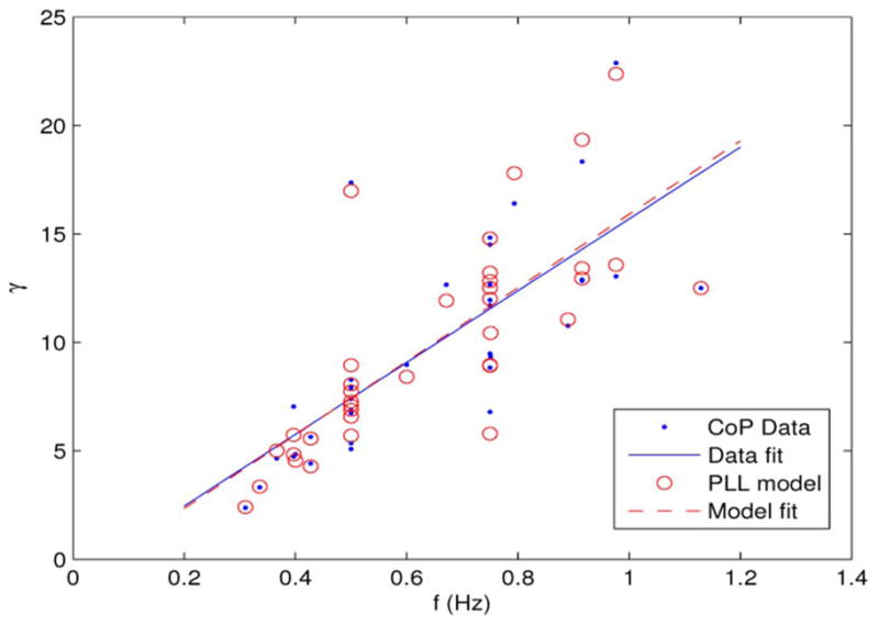
Amplitude gain, γ = B/A, for the CoP and the PLL model. The r2 value for the CoP linear regression is 0.57 and for the PLL linear regression is 0.59.
V. Discussion
A. PLL Observations
The proposed PLL model of the postural control system is based on the hypothesis that quiet standing CoP sway can be characterized as a weak sinusoidal oscillation that is corrupted with noise. Because the SNR of the QS oscillator is quite low (a mean of −17.4 dB), it is difficult to directly compute the characteristics of the oscillator from the QS sway itself. Instead, the frequency and amplitude of the QS oscillator can be inferred by examining how the oscillator responds to periodic motion of the platform. When the platform is driven by a sinusoidal stimulus, the QS oscillator changes speed until its frequency matches that of the platform, thus achieving phase lock. The observed phase lock behavior suggests an underling PLL mechanism that uses multiplicative feedback. The phase shift between the CoP sway and the moving platform can be used to determine the QS oscillator frequency, Fq, which corresponds to the center frequency of the PLL. Once the frequency is determined, the QS amplitude Aq can be computed using a least-squares fit. During phase lock, the observed phase shift is assumed to contain two components, one from a propagation delay τd in the neural, sensory, and motor systems, and the other from the PLL. The phase shift Δθ = θ + ωτd remaining after the effects of the propagation delay have been removed is referred to as the residual phase shift. For a PLL controller, the residual phase shift should depend on both the platform frequency ω and the platform amplitude A as in (15) as follows:
| (30) |
If the residual phase shift behavior is consistent with a PLL mechanism, a number of qualitative observations can be made.
Phase lock is possible only over a finite capture range of platform frequencies, ω.
The size of the capture range decreases with decreasing platform amplitude, A.
The residual phase shift decreases with increasing platform frequency. It is positive for ω < ωq, and becomes negative for ω > ωq.
The magnitude of the residual phase shift decreases with increasing platform amplitude.
Although the results of the phase lock experiments are not definitive, they do support these observations. Observations A and B postulate that there is a capture range, and that the capture range shrinks as the platform amplitude decreases. Evidence for this can be found by examining the cases in Table I where phase lock was not achieved. Subjects 3 and 5 failed to achieve phase lock in 50% of the trials. In both cases the frequencies at which this phase lock failed were at the low end, ω = ω1 and at the high end, ω = ωM. This is consistent with (30) where one would expect phase lock to fail as the phase shift approaches the boundary of the hold in range. The mean value of the platform amplitude for the failed phase lock trials was A = 0.53 mm in comparison with an overall mean platform amplitude of A = 1.08 mm. Again, this is consistent with the observation that the size of the capture range decreases as the platform amplitude decreases.
Observation C suggests that the sign of the residual phase shift depends on whether the platform frequency is below or above the PLL center frequency Fq. Support for this observation can be found in the plots of Δθ versus shown in Fig. 9. Most of the data and the least-squares fit for the case F = 0.5 Hz are positive. This is consistent with F < Fq when the mean value of Fq = 0.69 Hz is used. Similarly, most of the data points and the least-squares fit for the case F = 0.75 Hz are negative. Observation D suggests that the magnitude of the residual phase shift should decrease as the platform amplitude increases. The least-squares trend lines in Fig. 9 are consistent with this observation as well, although it is acknowledged that there is considerable variation in the data.
Fig. 9.
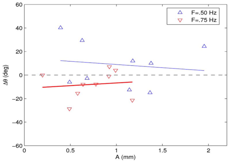
Residual phase shift versus the amplitude of the sinusoidal platform motion for two frequencies.
The method used to identify the parameters of the PLL model assumed that the QS oscillator is a weak sinusoidal oscillation whose characteristics are difficult to directly measure because of the significant noise present in QS sway. The indirect approach to determining Fq has the advantage that it allows one to set the quiet standing frequency such that the PLL has zero phase shift when the measured residual phase shift is zero, as was done in (22). An alternative approach is to apply cross correlation to the quiet standing data to find Fq using (7), similar to what was done for the periodic stimulus case. This leads to a mean QS frequency of Fq = 0.54 Hz. This approach yields the same qualitative results in terms of how the predicted phase varies with frequency. However, the observed phase shift and the PLL model will no longer be constrained to agree when the stimulus frequency equals Fq. The indirect approach to finding Fq that has been proposed here has the additional advantage that it does not rely on the quiet standing sway having a single distinct peak in its power density spectrum. In some instances a distinct single peak in the quiet standing sway is observed, but in other cases it is not.
Besides a QS oscillator, the other structural feature that separates the PLL model from linear feedback models is multiplicative feedback followed by low pass filtering. Realization of a multiplier type mechanism for phase detection might be achieved through modulated transmission of information across synapses. For example, if a QS oscillation opens different types of ion channels, alternating between excitatory and inhibitory post synaptic potential, then this could have a multiplicative feedback effect on the neural pathway that senses platform movement. Since the speed with which the overall system can respond is limited, this limited bandwidth will contribute to a low pass filtering of the multiplier output.
B. Nonlinear Effects
Many of the models that have been proposed for the postural control system are linear. However, time-varying and nonlinear effects have been reported. In [26] it was observed that the gain decreased with increasing stimulus amplitude. This phenomenon was not observed here, probably because the stimulus amplitudes were kept very small. They were set using psychophysical threshold levels making it more likely that one would be operating in the linear region. However, even when the periodic stimulus amplitude is kept small, nonlinear and time varying effects can be observed. For example, Loughlin and Redfern [27] have shown that both young and old healthy subjects adapt to constant frequency visual perturbations. Latt et al. [18] reported experimental results that violate the principle of superposition. The periodic stimulus used was galvanic vestibular stimulation (GVS) instead of platform movement. The responses measured included lateral CoP motion and head motion. The observed nonlinear behavior was in response to a dual frequency input consisting of two sinusoidal components, one at F1 = 0.1 Hz and one at F2 = 0.45 Hz. Although each of these periodic components, when applied separately, generated a distinct peak in the power density spectrum at the input frequency, the dual frequency stimulus did not produce a pair of peaks as would be expected with superposition, but instead only contained a peak at F2. The proposed PLL model is nonlinear due to the presence of multiplicative feedback. To demonstrate that similar qualitative behavior is possible, the PLL model was driven with the inputs u1(k) = 2 cos(2πF1kT), u2(k) = 2 cos(2πF2kT)and u3(k) = u1(k) + u2(k) with F1 = 0.5 Hz and F2 = 0.9 Hz. The power density spectra (PDS) of the CoP for the three cases are shown in Fig. 10. The PDS were computed using Welch’s modified average periodogram method with overlapping subsequences and a Hamming window. Clearly, the principle of superposition is not satisfied in Fig. 10 with the peak at F2 = 0.9 Hz attenuated in the dual-frequency response. For the PLL model, this phenomenon has a relatively simple explanation. The PLL locked onto the first of the two sinusoidal components of the stimulus. Similar behavior can be observed with other pairs of frequencies. The pair chosen in Fig. 10 was selected to lie on both sides of Fq and have a noninteger ratio. The dual frequencies F1 = 0.1 Hz and F2 = 0.45 Hz used in [18] also can be used if appropriate parameter values are selected for the PLL model. The PLL parameter values used in Fig. 10 were those of subject 7 in Table I.
Fig. 10.

Power density spectra of the PLL output for single-frequency and dual-frequency sinusoidal inputs of amplitude A = 2 mm.
C. Platform Movement Studies
A number of experimental studies have been reported that include platform perturbations. Peterka [26] used pseudo random rotations of the support surface and the visual surround, with and without sway referencing. The stimulus frequency range was [0.017, 2.23] Hz, and the amplitude range was [0.5, 8]°. A multichannel model (visual, vestibular, proprioceptive inputs) based on continuous feedback with PID control plus passive control of an inverted pendulum was proposed. For a fixed stimulus amplitude, the postural control system appeared to behave in a linear fashion, but nonlinear saturation effects were observed when the stimulus amplitude increased. It was shown that the nonlinear effects could be accounted for by changing the relative weighting of the three sensory input channels as a function of the stimulus amplitude with vestibular cues showing increased importance for large stimuli. Kooij and Vlugt [14] employed pseudo random periodic translations of a platform in the ML direction with platform frequencies in the range [0.05, 4.5] Hz. Using spectral analysis, the CoM and ankle torque responses were decomposed into periodic and remnant (stochastic) components. The results supported the conclusion that balance control is based on a continuous feedback mechanism where observed variations in the responses are due to noise associated with state estimation errors. Jeka et al. [28] used a periodic ML movement of a finger touch plate contact surface as a stimulus, and ML head position, CoM, and CoP as responses. Frequencies in the range [0.1, 0.8] Hz and amplitudes in the range [2.25, 18] mm were used. Based on observed phase lags, it was concluded that both position and velocity feedback are used for postural control.
The experimental studies in [14], [26], [28] as well as simular studies involving vestibular perturbation [29], [30] and visual perturbation [31] all measurement frequency response characteristics using broadband stimuli. Because the PLL model is nonlinear and therefore does not obey the principle of superposition, a broadband stimulus can not be used to directly measure its frequency response. However, using sinusoidal inputs whose frequencies and amplitudes lie within the capture range of the PLL, the frequency response can be determined in a point-wise fashion by measuring the gain and phase shift of the sinusoidal component of the steady state response. For the range of stimulus frequencies used here, [0.3, 1.1] Hz, [26] reported a magnitude response that was approximately flat with the gain beginning to fall off beyond 1 Hz. This is in contrast to the composite magnitude response shown in Fig. 8 where the gain increases with frequency over the measured range. The discrepancy is perhaps due to the different types and sizes of stimuli used (large pseudo random tilting platform versus small sinusoidal translating platform) which make a direct comparison difficult. In [14] a translating platform was used and in this case the gain (normalized to gravitational stiffness) did increase with frequency similar to that observed in Fig. 8. Likewise, the CoP gain increased with frequency in [28].
The phase information reported here agrees quite closely with that observed in [14], [26], and [28]. In each case it was observed that for low frequencies there is a small phase lead, and as the stimulus frequency increases this causes a large phase lag characteristic of a time delay. The time delay, τd, reported in [26] varied with the stimulus amplitude and ranged from a mean of 191 ms for a 0.5° stimulus to 105 ms for an 8° stimulus. For the PLL model a mean time delay of τd =260 ms was found. Recalling that only low amplitude (psychophysical threshold) stimuli were used, this appears to agree reasonably well. It is important to note that the residual phase shift component generated by the PLL does produce a phase lead at low frequencies as can be seen in Fig. 9. Consequently, a small low frequency phase lead accompanied by a large high frequency phase lag is consistent with the proposed PLL model.
D. Conclusions
The PLL model presented here is a nonlinear model that does not obey the principle of superposition. This is a limitation of the proposed model because broadband inputs can not be used to directly measure the frequency response characteristic as they can with linear models. Instead, the frequency response can only be measured in a pointwise fashion over the capture range of the PLL. The absence of superposition is also a strength because the PLL model successfully predicts nonlinear behavior observed in a dual frequency experiment reported previously in [18] (albeit using a different type of stimulus). Another useful feature of the proposed PLL control mechanism is that it suggests a number of qualitative characteristics (items A–D) that can be tested directly in future experiments. The PLL model reported here was identified and tested using experimental data obtained from nine healthy young adults. The data from these subjects represents legacy data in that the primary focus was the measurement of psychophysical threshold values for small sinusoidal movements of the platform. It also included supplementary quiet standing and phase lock experiments at four frequencies and four amplitudes, and these provided sufficient data to identify and test a PLL model. The authors are in the process of designing additional experiments using a larger range of frequencies and amplitudes applied to a wider group of subjects including older subjects so that changes in the parameters of the PLL model with age might be investigated. Preliminary indications suggest that older subjects who are less steady may exhibit more phase shift and fall out of phase lock sooner than younger subjects with superior balance. However, it remains to be determined if this is actually the case. If the phase shift associated with a low amplitude sinusoidal stimulus can be measured quickly and reliably, then this technique might potentially provide an alternative way to assess steadiness [32].
Acknowledgments
The authors would like to thank G. Fulk, J. Xu, C. M. Storey, X. Dong, R. B. Pilkar, V. B. Bhatkar, and past members of the SLIP-FALLS group for their help. The authors would also like to thank all of the Ph.D., M.S., and B.S. students in the SLIP-FALLS laboratory who helped in data collection over a number of years.
The work of C. J. Robinson was supported by a VA Senior Rehabilitation Research Career Scientist Award. Data collection was supported by a VA Rehab R&D under Grant E2143PC. Later data analysis was supported by NIH R01AG026553 and by a Coulter Foundation endowment to Clarkson University.
Biographies
Robert J. Schilling (SM’89) received the B.E.E. degree in electrical engineering from the University of Minnesota, Minneapolis, in 1969 and the M.S. and Ph.D. degrees in electrical engineering from the University of California, Berkeley, in 1970 and 1973, respectively.
He was a Lecturer in the Department of Electrical Engineering and Computer Science at the University of California, Santa Barbara, from 1974 to 1978. In 1978, he jointed the Department of Electrical and Computer Engineering at Clarkson University in Potsdam, NY, where he is currently a full Professor. He has authored four textbooks in the areas of engineering analysis, robotics, numerical methods, and digital signal processing. His current research interests include adaptive signal processing, active noise control, and control and identification of nonlinear systems.

Charles J. Robinson (F’91) received the B.S. degree in engineering science from the Franciscan University of Steubenville, the M.S. degree in electrical engineering from Ohio State University, and the D.Sc. degree in electrical engineering from Washington University, where he also trained as a biomedical engineer and a neuroscientist. He also held a post-doctoral position in Anesthesiology at Yale University.
He is the Shulman Chair of Rehabilitation Engineering at Clarkson University and Director of its Center for Rehabilitation Engineering, Science and Technology. Robinson also is a Senior Rehabilitation Research Career Scientist (SRRCS) with the U.S. Department of Veterans Affairs in Syracuse, NY, and was the first VA SRRCS to be selected in the country. He has been with the VA Research Service for almost 28 years, with postings in Chicago, Pittsburgh, Shreveport, and Syracuse. He taught in bioengineering programs at the University of Illinois-Chicago, the University of Pittsburgh, and Louisiana Tech University, where he was the Watson Eminent Scholar Chair in Biomedical Engineering and Micromanufacturing. He has held full Professor appointments in various clinical departments, including Neurology (Loyola), Orthopedic Surgery (Pitt and LSUHSC-Shreveport), and Physical Medicine and Rehabilitation (SUNY Upstate—Syracuse), and founded and chaired the Department of Rehabilitation Science and Technology at Pitt.
He is a Millennium Medalist of the IEEE.
Contributor Information
Robert J. Schilling, Email: schillin@clarkson.edu, Department of Electrical and Computer Engineering, Clarkson University, Potsdam, NY 13699 USA.
Charles J. Robinson, Rehabilitation Research Career, Syracuse VA Medical Center, Research Service 151, Syracuse, NY 13210 USA. He is also with the Center for Rehabilitation Engineering, Science and also with the Technology (CREST), Clarkson University, Potsdam, NY 13699 USA.
References
- 1.Prieto TE, Myklebust JB, Hoffmann RG, Lovett EG, Myklebust BM. Measures of postural steadiness: Differences between healthy young and elderly adults. IEEE Trans Biomed Eng. 1996 Sep;43(9):956–966. doi: 10.1109/10.532130. [DOI] [PubMed] [Google Scholar]
- 2.Diener HC, Dichgans J, Pompeiano O, Allum JHJ, editors. Progress Brain Res. Vol. 76. 1988. On the role of vestibular, visual, and somatosensory information for dynamic postural control in humans; pp. 253–262. [DOI] [PubMed] [Google Scholar]
- 3.Winter DA, Prince F, Frank JS, Powell C, Zabjek KF. Unified theory regarding A/P and M/L balance in quiet standing. J Neurophysiol. 1996;75:2334–2343. doi: 10.1152/jn.1996.75.6.2334. [DOI] [PubMed] [Google Scholar]
- 4.Rougier PR. Relative contribution of the pressure variations under the feet and body weight distribution over both legs in the control of upright stance. J Biomechan. 2007;40:2477–2482. doi: 10.1016/j.jbiomech.2006.11.003. [DOI] [PubMed] [Google Scholar]
- 5.Winter DA. Human balance and posture control during standing and walking. Gate Posture. 1995;3(4):193–214. [Google Scholar]
- 6.Corbeil P, Simoneau M, Rancourt D, Tremblay A, Teasdale N. Increased risk of falling associated with obesity: Mathematical modeling of postural control. IEEE Trans Neural Syst Rehabil Eng. 2001 Jun;9(2):126–136. doi: 10.1109/7333.928572. [DOI] [PubMed] [Google Scholar]
- 7.Bottaro A, Yasutake Y, Nomura T, Casadio M, Morasso P. Bounded stability of the quiet standing posture: An intermittent control model. Human Movement Sci. 2008;27(3):473–495. doi: 10.1016/j.humov.2007.11.005. [DOI] [PubMed] [Google Scholar]
- 8.Johansson R, Magnusson M, Akesson M. Identification of human postural dynamics. IEEE Trans Biomed Eng. 1988 Oct;35(10):858–869. doi: 10.1109/10.7293. [DOI] [PubMed] [Google Scholar]
- 9.Corradini ML. Early recognition of postural disorder in multiple sclerosis through movement analysis: A modeling study. IEEE Trans Biomed Eng. 1997 Nov;44(11):1029–1038. doi: 10.1109/10.641330. [DOI] [PubMed] [Google Scholar]
- 10.Winter DA, Patla AE, Riedtyk S, Ishac M, Winter DAM. Ankle muscle stiffness in the control of balance during quiet standing. J Neurophysiol. 2001;85:2630–2633. doi: 10.1152/jn.2001.85.6.2630. [DOI] [PubMed] [Google Scholar]
- 11.Casadia M, Morasso P, Sanguineti C. Direct measurement of ankle stiffness during quiet standing: Implications for control modeling and clinical application. Gait Posture. 2005;21:410–424. doi: 10.1016/j.gaitpost.2004.05.005. [DOI] [PubMed] [Google Scholar]
- 12.Loram ID, Lakie M. Direct measurement of human ankle stiffness during quiet standing: The intrinsic mechanical stiffness is insufficient for stability. J Physiol. 2002;545(1):1041–1053. doi: 10.1113/jphysiol.2002.025049. [DOI] [PMC free article] [PubMed] [Google Scholar]
- 13.Morasso P, Sanguineti V. Ankle stiffness alone cannot stabilize upright standing. Journal of Neurophysiology. 2002;88:2157–2162. doi: 10.1152/jn.2002.88.4.2157. [DOI] [PubMed] [Google Scholar]
- 14.van der Kooij H, de Vlugt E. Postural responses evoked by platform perturbations are dominated by continuous feedback. J Neurophysiol. 2007;98:730–743. doi: 10.1152/jn.00457.2006. [DOI] [PubMed] [Google Scholar]
- 15.Masani K, Vette AH, Popovic MR. Controlling balance during quiet standing: Proportional and derivative controller generates preceding motor command to body sway position observed in experiments. Gate Posture. 2006;23:164–172. doi: 10.1016/j.gaitpost.2005.01.006. [DOI] [PubMed] [Google Scholar]
- 16.Peterka RJ. Postural control model interpretation of stabilogram diffusion analysis. Biol Cybern. 2000;83:335–343. doi: 10.1007/s004220050587. [DOI] [PubMed] [Google Scholar]
- 17.Bottaro A, Casadio M, Morasso P, Sanguineti V. Body sway during quiet standing: Is it the residual chattering of an intermittent stabilization process? Human Movement Sci. 2005;24:588–615. doi: 10.1016/j.humov.2005.07.006. [DOI] [PubMed] [Google Scholar]
- 18.Latt LD, Sparto PJ, Furman JM, Redfern MS. The steady-state postural response to continuous sinusoidal galvanic vestibular stimulation. Gate Posture. 2003;18:64–72. doi: 10.1016/s0966-6362(02)00195-9. [DOI] [PubMed] [Google Scholar]
- 19.Gardner FM. Phaselock Techniques. 3. New York: Wiley; 2005. [Google Scholar]
- 20.Richerson SJ, Faulkner LW, Robinson CJ, Redfern MS, Prucker MC. Acceleration threshold detection during short anterior and posterior perturbances of a translating platform. Gate Posture. 2003;18:11–19. doi: 10.1016/s0966-6362(02)00189-3. [DOI] [PubMed] [Google Scholar]
- 21.Robinson CJ, Purucker MC, Faulkner LW. Design, control, and characterization of a sliding linear investigative platform for analyzing lower limb stability (SLIP-FALLs) IEEE Trans Rehabil Eng. 1998 Sep;6(3):334–350. doi: 10.1109/86.712232. [DOI] [PubMed] [Google Scholar]
- 22.Bhatkar VV, Pilkar RB, Storey CM, Robinson CJ. Amplitude demodulation of entrained sway to analyzer human postural control. Proc. 29th Intern. Conf. IEEE EMBS; Lyon, France. Aug. 23–26, 2007; pp. 4923–4926. [DOI] [PMC free article] [PubMed] [Google Scholar]
- 23.Kiemel T, Oie K, Jeka JJ. Multisensory fusion and the stochastic structure of postural sway. Biol Cybern. 2002;87:262–277. doi: 10.1007/s00422-002-0333-2. [DOI] [PubMed] [Google Scholar]
- 24.Haykin S. Adaptive Filter Theory. 4. Upper Saddle River, NJ: Prentice Hall; 2002. [Google Scholar]
- 25.Sparto PJ, Jasko JG, Loughlin PJ. Detecting postural responses to sinusoidal sensory inputs: A statistical approach. IEEE Trans Neural Syst Rehab Eng. 2004 Sep;12(3):360–366. doi: 10.1109/TNSRE.2004.834203. [DOI] [PMC free article] [PubMed] [Google Scholar]
- 26.Peterka RJ. Sensorimotor integration in human postural control. J Neurophysiol. 2001;88:1097–1118. doi: 10.1152/jn.2002.88.3.1097. [DOI] [PubMed] [Google Scholar]
- 27.Loughlin PJ, Redfern MS. Spectral characteristics of visually induced postural sway in healthy elderly and healthy young subjects. IEEE Trans Neural Syst Rehabil Eng. 2001 Mar;9(1):24–30. doi: 10.1109/7333.918273. [DOI] [PubMed] [Google Scholar]
- 28.Jeka J, Oie K, Schoner G, Dijkstra T, Henson E. Position and velocity coupling of postural sway to somatosensory drive. J Neurophysiol. 1998;79:1661–1674. doi: 10.1152/jn.1998.79.4.1661. [DOI] [PubMed] [Google Scholar]
- 29.Firzpatrick R, Burke D, Gandevia SC. Loop gain of reflexes controlling human standing measured with the use of postural and vestibular disturbances. J Neurophysiol. 1996;75(5):3994–4008. doi: 10.1152/jn.1996.76.6.3994. [DOI] [PubMed] [Google Scholar]
- 30.Johansson R, Magnusson M, Fransson PA, Karlberg M. Multi-stimulus multi-response posturography. Math Biosci. 2001;174:41–59. doi: 10.1016/s0025-5564(01)00075-x. [DOI] [PubMed] [Google Scholar]
- 31.Kiemel T, Elahi AJ, Jeka JJ. Identification of the plant for upright stance in humans: multiple movement patterns from a single neural strategy. J Neurophsiol. 2008;100:3394–3406. doi: 10.1152/jn.01272.2007. [DOI] [PMC free article] [PubMed] [Google Scholar]
- 32.Bollt EM, Fulk GD, Skufca JD, Al-Ajloluni AF, Robinson CJ. A quiet standing index for testing the postural sway of healthy and diabetic adults across a range of ages. IEEE Trans Biomed Eng. 2009 Feb;56(2):292–302. doi: 10.1109/TBME.2008.2003270. [DOI] [PMC free article] [PubMed] [Google Scholar]