

Abstract
Researchers studying complex cognition have grown increasingly interested in mapping symbolic cognitive architectures onto subsymbolic brain models. Such a mapping seems essential for understanding cognition under all but the most extreme viewpoints (namely, that cognition consists exclusively of digitally implemented rules; or instead, involves no rules whatsoever). Making this mapping reduces to specifying an interface between symbolic and subsymbolic descriptions of brain activity. To that end, we propose parameterization techniques for building cognitive models as programmable, structured, recurrent neural networks. Feedback strength in these models determines whether their components implement classically subsymbolic neural network functions (e.g., pattern recognition), or instead, logical rules and digital memory. These techniques support the implementation of limited production systems. Though inherently sequential and symbolic, these neural production systems can exploit principles of parallel, analog processing from decision-making models in psychology and neuroscience to explain the effects of brain damage on problem solving behavior.
Keywords: problem solving, production system, neural network, diffusion, decision making, symbolic, subsymbolic
1. Introduction
In order to build biologically plausible cognitive models that exhibit the full range of human behavior — from playing chess to balancing on skates — it seems that researchers will inevitably require models that can implement finite state automata (e.g., for representing and executing sequences of chess moves), and at the same time, feedback controllers for dynamical systems (e.g., for correcting a destabilizing wobble). Similarly, it will almost surely require models that are robust to perceptual noise, but that can behave stochastically when desired; and that require no central clock to govern synchronous, digital circuitry, but that can still time intervals and represent symbols.
We present a technique for building cognitive models that may be able to satisfy the disparate and seemingly paradoxical requirements outlined above. This technique draws on the strengths of existing symbolic (or quasi-symbolic) cognitive architectures, such as Soar (Laird et al., 1987) and ACT-R (Anderson and Lebiere, 1998) among others, but it implements every feature in a physical-level design that di ers substantially from the design of standard computer hardware. It also draws on the strengths of existing subsymbolic cognitive models, including models of associative memory and of decision making.
Using this technique amounts to hardwiring neural networks to produce complex models of approximately symbolic processing. What is left out of this hardwiring approach, of course, is one of the primary virtues of neural networks — the simple and powerful learning algorithms that can be applied to them (e.g., Rumelhart et al., 1986; Ackley et al., 1985; Williams and Zipser, 1989; Sutton and Barto, 1998). Our hope, however, is that in showing how a hardwired system may resolve some of the differences between strictly symbolic and strictly subsymbolic cognitive models, we will have presented a well-defined target architecture that future learning algorithms may be designed to acquire through experience.
To best achieve our purpose, and to show that an account of a symbolic / subsymbolic interface can have practical consequences in cognitive modeling, this paper investigates the functionality underlying human problem solving. Problem solving has been argued to exemplify complex cognition (Miller et al., 1960; Newell and Simon, 1972), but it is not typically modeled with neural networks (although see Dehaene and Changeux, 1997). While what we present is by no means a comprehensive theory of human problem solving, we hope that it illustrates the leverage that can be gained from extracting symbolic processing out of a subsymbolic system.
We begin from the same starting point assumed in some of the earliest cognitive modeling efforts: namely, we model problem solving as a process of heuristic search (Newell and Simon, 1963). However, our approach differs from early symbolic modeling efforts in that it does not presuppose any hard and fast distinction between software and hardware. Instead, it directly addresses a lower level of description whose fundamental atoms we propose to be standard, artificial neural network units. We choose this level of description despite the fact that it, like a purely symbolic approach itself, sacrifices a great deal of biophysical detail. We note at the outset, however, that there is growing evidence that this type of neural network may plausibly be reduced even further to models whose greater level of physical detail is more appropriate to single-cell physiology than to whole-brain function (Wang, 2002; Wong and Wang, 2006).
In what follows, we build from this model of the physical processing level up to an architecture capable of problem-space search, presenting possible solutions to problems that arise along the way. Admittedly, this is an architecture with several limitations — including an inability to implement firstorder logic — that all appear to reduce to what is commonly known as “the binding problem”, and which further work must address. However, a variety of promising approaches to this problem already exist that seem compatible with the proposed architecture, including the binding of object features through temporal synchrony of activations (Shastri and Ajjanagadde, 1993) — an approach which supports analogical reasoning in some systems (Hummel and Holyoak, 1997) — and, without relying on synchrony, using layers of conjunctive processing units (O’Reilly and Busby, 2002) to bind features. The general problem of using neural networks to represent first-order logic statements and to carry out deductive inference has also been addressed by a number of approaches, several of which are detailed in Hammer and Hitzler (2007).
The organization of the paper parallels both the design-level hierarchy of modern computer engineering (Hayes, 1993) and the levels-of-analysis hierarchy made famous by David Marr in vision research (Marr, 1982). Section 2 covers the basic ‘physical-level’ (Hayes, 1993) or ‘implementational-level’ (Marr, 1982) building block that we will use for cognitive modeling — a stochastic version of a classic artificial neural network unit. Section 3 covers the decision making networks that form the basic components of the architecture’s ‘logic level’, in engineering terms. Sections 4 and 5 cover the composition of these networks into sequential processing systems equivalent to simple production systems (collections of if-then rules coupled with a working memory). Because of their computational power and psychological plausibility, production systems are used widely in symbolic cognitive modeling (e.g. Anderson and Lebiere, 1998; Just and Carpenter, 1992; Laird et al., 1987; Kieras and Meyer, 1997).
In order to demonstrate the usefulness of a well-specified symbolic/subsymbolic interface for cognitive modeling, section 6 reviews published results from a model that incorporates this interface. We applied it to human performance data from a problem solving task used in psychology to assess cognitive deficits in brain damage and disease (the Tower of London task of Shallice, 1982). These sections correspond to the ‘architecture level’ in engineering and span the implementational and ‘algorithmic’ levels in Marr (1982); they provide most of the essential pieces of a cognitive architecture — that is, a framework of core assumptions that defines a space of possible cognitive models (Newell, 1990).
We conclude with a general discussion in section 7. In the supplementary materials, we give a specification of the previously mentioned cognitive model of human performance in the Tower of London task (the details of which have not been published and may interest modelers seeking to replicate or generalize our modeling results). This example serves as an existence proof that recurrent neural networks may serve as a bridge between low-level, biophysically detailed neuron models and high-level psychological models.
2. Basic building block
In this section, we define a stochastic version of a classical model of neural population activity that has received empirical support from neurophysiology (e.g., Shadlen and Newsome, 1998). This population model will serve as the basic building block of a proposed cognitive architecture. In its deterministic form (cf. Cohen and Grossberg, 1983; Hertz et al., 1991; Hopfield, 1984; Lapique, 1907; Wilson and Cowan, 1972), this simple model feeds a linear combination of a unit’s inputs into a system defined by one of the simplest possible nonlinear differential equations. It is formally equivalent to an electric circuit of resistive inputs feeding into a capacitor, or leaky integrator, whose output is boosted by an operational amplifier (Mead, 1989).
Computing linear combinations or weighted sums of inputs allows a model neural population to perform arbitrary linear transformations of its inputs. This capability has proven useful for modeling fundamental human learning and categorization capacities by a number of authors (e.g., Anderson et al., 1977; Rosenblatt, 1958). It will form the basis of our subsymbolic approach to simple decision making in section 3 and to more complex decision making in section 5, where we equate making a decision to voting for outcomes in an election. Further, it is consistent with the basic phenomena in synaptic transmission between neurons, which lend themselves well to a linear description if plasticity is not too great (Dayan and Abbott, 2001). Importantly, a linear model for integrating multiple inputs also has the advantage of allowing the large body of linear systems theory to aid in the formal analysis of models. Subsequently transforming these linear combinations with a nonlinear tranformation (namely a squashing function) then allows a tremendous increase in functionality (such as the ability to represent any continuous function; see, e.g., Bishop, 2006) without a complete loss of analytical tractability.
In addition to the linear combination of momentary inputs, the model assumes the addition of Gaussian noise to these inputs, followed by leaky integration of these noise-corrupted combinations from moment to moment prior to application of the nonlinear transformation. Leaky integration is formally defined in appendix A, where we also discuss the stochastic numerical integration technique used to simulate the proposed architecture on a computer.1 Similar behavior occurs in a resistor-capacitor (RC) circuit: when the input voltage to such an RC circuit is abruptly changed, the output voltage approaches the new value at an exponential rate determined by the value of the circuit’s time constant, which equals the inverse of the resistance times the capacitance (Oppenheim and Willsky, 1996).
It is from this property that we derive two of the most important reasons to use this stochastic model. One is functional, which is that the RC factor (equivalently, the time constant) determines the model’s ability both to act as a low-pass filter — that is, to filter out high-frequency noise — and to act as a short-term memory. Thermal noise occurs at roughly equal power at all frequencies in electrical circuits (Gardiner, 2004), and is therefore referred to as ‘white’ noise. In contrast, most signals of interest will have an upper frequency bound, leaving a high-frequency band filled entirely with noise. Thus, attenuating high frequencies is probably critical for the survival of organisms that use electrical activity to process information. At least a small amount of such attenuation is, in any case, probably unavoidable in any physically implemented system: the small capacitances in digital, sequential circuits provide a small amount of noise reduction, for example.2 When applied to Gaussian signals corrupted by Gaussian white noise, this approach to filtering is in fact equivalent to the optimal Bayesian signal estimation procedure (Poor, 1994); when it is not optimal, it can frequently still approximate such a procedure, and unlike a true Bayesian approach, it requires no explicit priors and is computationally tractable under all circumstances. Furthermore, noise allows random behavior, which is essential in competitive games (Von Neumann and Morgenstern, 1944).
The other major reason for using this model is empirical, since individual neurons themselves have a capacitive membrane with resistive conducting pores (Hodgkin and Huxley, 1945). Thus leaky integration is known to occur in the brain (albeit in the context of a variety of more complex processes). Simple, leaky integrators can be related to more complex models of neural activity (Gerstner, 2000; Wang, 2002; Wong and Wang, 2006) that can in turn be related to the widely accepted model of Hodgkin and Huxley (1952), but the simplicity of leaky integrator models allows analytical solutions that more complex models lack.
As we discuss in the next section, however, the time constant of individual neurons is much too small to provide the kind of noise filtering and slow memory decay that may be required for typical cognitive tasks (instead, individual neurons appear to be optimized for millisecond-level computation). Nevertheless, populations of neurons acting in concert may be able to achieve time constants that are much larger than that of an individual neuron (Wang, 2001). In addition, Seung et al. (2000) discuss a method that we review here for using recurrent, self-excitatory feedback within such a population to achieve an arbitrarily large time constant, including an ‘infinite’ time constant that causes a self-exciting unit to act as a perfect integrator of its inputs (see Eq. 20). This fact will allow us to design mechanisms that time intervals and provide feedback control with desirable properties (namely, properties that allow cognitive models to make decisions robustly). These mechanisms in turn will enable the construction of models that carry out problem space search without the use of a central, oscillating clock and a traditional, synchronous circuit design.
Obviously, electric circuit models also describe electrical activity in the type of hardware underlying programmable computers. As a result, a single form of mathematics can be used for our ultimate goal of linking psychological models to neurophysiological models, and also for translating between the symbolic computational level and the physical level of transistors, resistors and capacitors in modern computing technology.
Formally, a low-pass filter coupled with a nonlinear activation function forms a system defined by a stochastic differential equation (SDE), Eq. 1, and a squashing function, Eq. 2:
| (1) |
| (2) |
Here, V is taken to represent the average firing rate of a neural population; λ determines the slope of the sigmoidal activation function f, and β represents the offset voltage, or equivalently, the value of the input x such that f(x) = 0.5. By arguments in Appendix B, however, we can use a single, much more manageable equation with approximately the same behavior (cf. Cohen and Grossberg, 1983):
| (3) |
Here I represents a weighted sum of inputs from other units: . The variable c’ represents the weighted sum of noise terms, which averages out to 0 in the limit of a large number of uncorrelated noise terms.
Now we turn to compositions of these building blocks for carrying out an essential operation in both computer technology and human and animal behavior: namely, decision making.
3. Composition of decision making circuits
With basic computing elements in hand, we now describe an implementation of symbols and logical rules. Symbols arise in our analog system through a quantization (Gray and Neuhoff, 1998) or categorization process. The particular categorization process we use is equivalent to a well-supported model of decision making in psychology and neuroscience known as the diffusion (or drift-diffusion) model (cf. Ratcliff, 1978), which itself is inspired by the physics of Brownian motion (Gardiner, 2004). A ‘decision’ is the selection of a unique outcome from among a finite or countably infinite set of discrete possibilities, although the inputs to such a process are often continuous.
This quantization approach is also at the heart of basic decision-making operations in digital electronics (and in symbolic cognitive modeling approaches like production systems). Decisions are the fundamental logic-level operations that allow a purely symbolic (i.e., binary) description of the physical state of a circuit and a description of its dynamics in terms of propositional logic, even though the physical laws governing its behavior are defined by differential equations and continuously varying quantities. Applying logical operations to symbolic descriptions then allows engineers to design at the hierarchically higher architecture level (and software engineers to program at a still higher level) using much simpler Boolean algebra. We hypothesize that symbolic search processes arise in cognition for similar reasons of increased efficiency.
3.1. A standard voltage binarization scheme
Although we will argue that analog computation should not be ignored in cognitive modeling, the way in which standard computers implement digital behavior in inherently analog circuitry will nevertheless provide a paradigm for our own analog-to-digital (AD) conversions when they occur. Given that continuous change in the output voltage is produced by continuous change in the input voltage, all-or-none switching behavior in networks of transistors, resistors and capacitors is determined simply by choosing a convention for voltage levels that correspond to ‘all’ (1) and to ‘none’ (0). This convention assigns a band of acceptable voltage values for representing a 0 to small voltages, and a wider band of acceptable voltage values for representing a 1 centered at a higher voltage (Hayes, 1993). The conventions for transistor-transistor logic (TTL) circuits, which are used for a wide range of digital electronic circuits, are shown in Fig. 1.
Figure 1.

Voltage bands corresponding to 1 (voltages greater than 2), and 0 (voltages less than 0.8). These ranges define the limits for acceptable inputs to a logic gate. Output voltage criteria are stricter. Greater reliability is achieved when logic component manufacturers adhere to this scheme, because one gate in a chain can effectively clean up extreme noise in its inputs before propagating its output.
In a digital system, symbolic representation is achieved by the use of these bands. When the output voltage of a transistor-based logic gate falls within one band, it will be virtually guaranteed to produce an output in downstream components that also falls within one of these bands. The width of these bands is set so that noise cannot erroneously flip a bit, except in circumstances of very small probability (and error-checking schemes are built in to digital circuits to further reduce this probability). Noise is an ever-present element of real, electronic system operation due, among other reasons, to the heat generated by electric current flowing through resistive material. Dealing with this noise when we abandon a digital interpretation of voltages is of major importance.
In a noisy environment, the task of detecting whether a signal is present can be non-trivial. The same is true inside an electronic system that does not adhere at all times to a TTL voltage scheme (i.e., one that combines analog and digital circuitry). When many signals are possible, and evidence for each conflicts with evidence for the others, the task of deciding on a signal’s identity is all the more difficult.
Fortunately, the study of signal detection and decision making that has taken place since the 1940s — in engineering, statistics and psychology — has led to a clear understanding of optimal performance in these tasks. It has also produced a rigorous analysis of various algorithms for carrying them out. A great deal of behavioral research in psychology has furthermore been devoted to examining these algorithms as models of human and animal decision making. As we will show, all of this work provides a strong incentive for choosing some variety of a random walk as our algorithm for signal detection and decision making. More fortunately still, recent work in psychology and neuroscience provides us with a simple mapping from these algorithms onto neural networks, our computational medium of choice (Bogacz et al., 2006).
In this section we draw on this work to develop an attractor network mechanism for resolving conflict between the possible outputs of a decision making element: this mechanism uses lateral inhibition to implement a process of competition between responses. Lateral inhibition is an old idea in neuroscience (Hartline and Ratliff, 1957) and neural networks (McClelland and Rumelhart, 1981; Grossberg, 1980b), and underlies many associative memory models based on attractor networks in psychology. We draw on this work to formalize our approach to the basic decision making operations of our system when ambiguous inputs attempt to produce more than one output from an element.
It is at this point that analog numerical representation begins to impact the method by which neural networks emulate finite state automata and production systems: unlike standard computer hardware components, individual units in a decision making element will now represent real numerical quantities of evidence using an analog code. Specifically, this code relates activation levels monotonically to the likelihood ratio of the hypotheses (or preferences) under consideration.
We now examine how theories of signal detection and decision making, particularly random walk models, contribute to our story. We will then be ready to address the implementation of productions and the resolution of conflict.
3.2. Theories of signal detection and decision making in statistics, psychology and biology
A great deal of psychological research has focused on the processes leading up to human responses in simple decision making tasks. Signal detection — the subject of psychophysical investigation since Weber in the early 1800s — involves a single response to stimuli of a single category. Signal discrimination or choice reaction — also studied since the 1800s using reaction time techniques developed by Donders — involves multiple stimulus classes and responses (Green and Swets, 1966). In our analysis, decision making will be taken to include these simple processes, as well as other, more complex processes leading to discrete responses (for example, choosing a car to purchase; cf. Roe et al., 2001). Our purpose in this section, though, is to situate the building blocks of a neural cognitive architecture in a framework that has recently connected neurobiological research on decision making to behavioral reaction time research (Smith and Ratcliff, 2004). For that reason, we will focus on the favored task in this domain: discrimination tasks involving two stimulus categories, each associated with its own response.
In this domain, models that employ a technique known as sequential sampling have been used to explain some widely observed features of response time (RT) and accuracy data (Luce, 1986) — in particular, the specific shape of the long-tailed RT distributions that typically occur in human reaction time experiments. In sequential sampling models, the stimulus is assumed to consist of a stream of samples from one of two probability distributions (Fig. 2A illustrates an example of two Gaussian distributions). To determine which distribution is actually generating the stimulus, the samples are accumulated over time. Evidence in favor of one or the other hypothesis thus builds up until a response criterion — or decision threshold — has been reached. Sequential sampling models explain speed-accuracy tradeoffs in decision making performance in terms of shifts in the response threshold toward or away from the starting point of the decision variable trajectory: closer thresholds produce shorter RTs and higher error rates on average (Grice, 1972; Laming, 1968; Ratcliff, 1978; Reddi and Carpenter, 2000).
Figure 2.

A: Two possible stimulus distributions; B: Four sample paths of a drift-diffusion process; C: Long-tailed analytical RT density (solid curve) and simulated RT histogram (top), correct RT histogram (middle), error RT histogram (bottom); D: Time courses of noise-free, mutually inhibitory evidence accumulation units with sigmoid activation functions and mutual inhibition of strength ξ; E: The sigmoid activation function; F: A smoothed sample path of mutually inhibitory accumulator activations in the (y1, y2)-phase space showing rapid attraction to a line (the ‘decision plane’) followed by drift and diffusion in its neighborhood.
In accumulator versions of sequential sampling models, evidence accumulates independently in a set of accumulators, one of which is assigned to each hypothesis. In random walk versions, in contrast, each sample that increases the evidence for one hypothesis (i.e., the likelihood of that hypothesis given the data) correspondingly reduces the evidence in favor of the other. This is a form of competition that effectively reduces two decision variables to one: this variable equals the difference in accumulated evidence for each hypothesis. (Fig. 2B shows the trajectory of this variable plotted against time for four different decisions superimposed on each other. Fig. 2C shows the resulting response time distributions over many decisions.)
The ratio of the likelihoods of the two hypotheses is the quantity that is implicitly used to make the decision in most random walk models: when the likelihood ratio approaches 0, the hypothesis corresponding to the denominator is almost certainly true; when the ratio approaches infinity, the hypothesis corresponding to the numerator is almost certainly true. Assuming independence of individual samples, the current likelihoods can be updated to incorporate a new sample quite easily: the likelihood of the hypothesis given the single sample is multiplied against the total likelihood of the hypothesis given all previous samples.
When the logarithm of the likelihood is taken, this multiplication becomes an addition. Similarly, dividing one likelihood by the other becomes subtraction when the logarithm of the ratio is taken. Steps in the random walk thus equal increments to the logarithm of the likelihood ratio for one hypothesis over the other. This property makes such a model equivalent to the sequential probability ratio test, or SPRT (Stone, 1960). This fact is encouraging for the use of random walk models, since the SPRT is optimal in a statistically stationary environment, in the sense that no other test can achieve higher expected accuracy in the same expected time; conversely, no other test can reach a decision faster for a given level of accuracy (Wald and Wolfowitz, 1948).
The drift-diffusion model (DDM) (Ratcliff, 1978) is a sequential sampling model in which stimuli are sampled continuously rather than at discrete intervals, like the continuous-time low-pass filter mechanism of Eq. 3 (we will soon review a proof that the DDM can in fact be approximated by a suitably organized neural network). With human subjects, the DDM has accounted for response time distributions and choice probabilities in a wide range of two-alternative tasks (Ratcliff and Rouder, 1998; Smith and Ratcliff, 2004).
During decision making by the DDM, the difference between the means of the two possible stimulus distributions (see Fig. 2A), imposes a constant drift of net evidence toward one threshold, and the variance imposes a Brownian motion that may lead tofferrors. The DDM is defined by the following stochastic differential equation (SDE):
| (4) |
We examined similar equations when discussing analog computation in section 2. Here, the equation is arguably simpler. A is the signal strength; when it is nonzero, it produces a tendency for trajectories x(t) to move, or ‘drift’, in the direction of the signal. Brownian motion produced by integrating a white noise process W, causes diffusion of a substance within a liquid — hence the term ‘diffusion’ in the name of the model. The factor c weights the intensity of this di usive component of x’s motion.
3.2.1. Sequential sampling by leaky integrator networks
In monkeys performing oculomotor tasks, the continuously evolving firing rates of neurons in the lateral intraparietal sulcus (area LIP) have been related to competing evidence accumulators that approximately implement a drift-diffusion process (Gold and Shadlen, 2001; Roitman and Shadlen, 2002; Shadlen and Newsome, 2001). Similar findings have been reported for frontal structures responsible for controlling eye movements (Hanes and Schall, 1996). We now examine how a network of leaky integrator units can implement the DDM in this way, thereby achieving nearly optimal decision making capabilities in addition to nearly optimal signal estimation capabilities in a way that is consistent with evidence from neuroscience.
Evidence accumulation can be approximated by a simple neural network with two leaky integrators, each of which responds preferentially to one of the stimuli. Each integrator is also subject to inhibition from the other integrator (see Fig. 2D), as proposed by Usher and McClelland (2001) (cf. Bogacz et al., 2006; Gold and Shadlen, 2002; Grossberg, 1982). The evolving activation of each unit (indexed by i) is determined by an SDE, the deterministic part of which is given by Eq. 5:
| (5) |
Eq. 5 is a version of the basic leaky integrator unit (Eq. 3) that is linearized for easier analysis. In this equation, Ii is the input to unit i. It is usually assumed to be a step function of time (corresponding to stimulus onset). The parameter ξ represents the inhibitory strength of symmetric connections between the two decision units; −ξyj represents inhibition from the other unit(s).
When noise is included, the pair of linearized units is governed by Eqs. 6-7:
| (6) |
| (7) |
Assuming linearity also allows us to make the relationship between the DDM and its neural network implementation explicit. By adding the two, noise-free, linearized equations (Eqs. 6-7), we get a quantity, yc = y1(t) + y2(t), that approaches an attracting line — defined in the (y1, y2) plane by y1 + y2 = (I1 + I2)/(1 + ξ) — exponentially at rate 1 + ξ. Subtracting the second equation from the first yields an Ornstein-Uhlenbeck process for the net accumulated evidence, x = y1 − y2:
| (8) |
We will refer to the attracting line as the ‘decision line’ (following Bogacz et al., 2006). The difference quantity, y1 − y2, represents movement along this plane in one of two possible directions. By using strongly self-exciting units to implement thresholds on the activation values, y1 and y2, decisions can be read out of this system. These thresholds define lines in the phase space of unit activations that intersect the decision plane (the dashed lines in Fig. 2F). These intersections are equivalent to decision thresholds applied to a process of drift and diffusion along the decision line.
If leakage and inhibition are balanced (ξ = 1), the drift term is a constant, A, and the system is equivalent to the DDM (Eq. 4) with A = I1 − I2 representing the difference in inputs (Brown et al., 2005; Holmes et al., 2005).
Fig. 2F shows the evolution of the activations y1(t) and y2(t) over time. After stimulus onset, the system state (y1, y2) approaches the decision plane. Projection of the state (y1, y2) onto this line yields the net accumulated evidence x(t), which approximates the DDM as shown in Fig. 2B. Fig. 3 shows that including nonlinear activation functions does not dramatically change the decision making dynamics.
Figure 3.
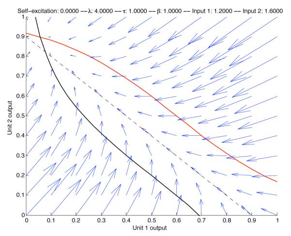
The phase portrait of a nonlinear two-unit system in which the decision plane is a good approximation of where decision making takes place. The red curve illustrates the isocline of zero vertical velocity, and the black curve represents the isocline of zero horizontal velocity. Thus, their intersection is a stable attractor. Here unit 1 is given a net input of 1.2, and unit 2 is given a net input of 1.6.
We have now addressed the evidence accumulation aspect of two-alternative decision making, but we have not addressed how a surplus of evidence in favor of one hypothesis is ‘read out’ into a decision. We must address this issue because of a conceptual problem: if a surplus of size x is sufficient for making a decision that in many cases leads to a motor action, then why is x−∊ not sufficient, for any ∊ > 0? How can an arbitrarily small change in the surplus make the difference between taking an action and remaining still? We can address this problem easily by adding a second layer of strongly self-exciting units that implement step functions (approximately). We discuss this solution in detail in section 4.
Thus, extremely simple leaky integrator units that provide nearly optimal signal estimation can also perform nearly optimal decision making in the context of difficult, two-alternative tasks.
3.3. Attractor and winner-take-all networks in higher dimensions
We have shown a simple example of an attractor network for the case of two-alternative decisions. The pair of threshold detector units used to detect threshold crossings in the accumulator/leaky integrator layer has four attractors in the state space of activations: both units near 0; one near 0 and the other near 1; and both near 1. Assuming normal operating conditions for a properly parameterized two-alternative decision making circuit, and assuming one of the two signals is present, the expected behavior is that ultimately, one of the two units will achieve an activation near 1, and the other will remain at an activation near 0. Thus, the system of two threshold units acts as a winner-take-all (WTA) network. This scheme can be generalized to n units and constitutes a 2-layer building block for a cognitive architecture that is analogous to the logic gates in computers.
We can also collapse the accumulator layer and the threshold layer of units into a single layer of self-exciting units, as in the model of Wong and Wang (2006). Analysis of the relationship between the SPRT and such models is not as well developed as for the two layer network, but such networks exhibit similar dynamics and may allow a simpler, one-layer building block.
Here we generalize this two-channel WTA network to n channels. Technically, depending on the interconnections among units, such a network could have an arbitrarily large number of attractors in the state space of possible activations of all units (Amit et al., 1985). However, we are only interested in attractors that we can easily use to do computation. Thus we will primarily investigate networks whose attractors under normal conditions consist of exactly n + 1 patterns of activation: one in which all units are near 0 activation, and for each of the n channels, one pattern in which the given channel’s threshold unit is near 1 while all the others are near 0 (i.e., a localist representation).
We can generalize beyond two dimensions by considering first three dimensions, defined by Eqs. 9:
| (9) |
A general, n-dimensional version of Eqs. 9 is a nonhomogeneous linear system that can be transformed into a system with 2 unique eigenvalues (of multiplicities 1 and n − 1) and n orthogonal eigenvectors (McMillen and Holmes, 2006). The eigenvalue of multiplicity 1 corresponds to the eigenvector , which defines the position of a decision plane — an n − 1-dimensional generalization of the 1-dimensional decision line in the two-alternative case. The remaining eigenvalues correspond to orthogonal directions within the decision plane that push the system toward a threshold on the plane.
Returning to the three-dimensional situation, let B = y1 +y2 + y3. Then Eqs. 9 imply Eq. 10:
| (10) |
Setting to 0 gives the following relationship between the three activation variables:
| (11) |
This defines a 2-dimensional decision plane that, like the 1-dimensional decision line in the two-alternative case, cuts diagonally through the activation bounding box. This intersection forms a triangular area (see the triangular surface in Fig. 22) within which drift and diffusion take place (McMillen and Holmes, 2006). The boundaries of the triangle are absorbing, meaning that as soon as the system hits one of them, the process stops. Thus they act as response thresholds in a decision making context. (The decision plane can also form a hexagonal bounding area with three absorbing and three reflecting boundaries, depending on the precise decision plane placement. Reflecting boundaries prevent the system from going beyond them, but do not stop the evolution of the process; thus the system can hit a reflecting boundary and then move back away from it over time.)
In general, we can continue this pattern for n alternatives to get a decision plane defined by Eq. 12:
| (12) |
We can always generate a winner by exciting one unit more strongly than all others by some margin. The problem is that we can also easily produce either no winner, or multiple winners, by carelessly defining input strengths and the connection strengths from the accumulator layer to the threshold layer. These problems are addressed in appendix C, where nonlinear, integral feedback control is used to ensure the WTA property of our decision making networks.
We now address the means by which connections and connection strengths can be programmed to implement competing if-then rules, or productions, of varying degrees of preference, as well as the state-maintenance and sequential state transitions that define a finite state automaton (FSA).
4. Sequential processing
We have discussed how a simple, low-pass filtering mechanism can be applied to the problem of signal estimation and decision making. We now address how a network of these mechanisms can emulate a memory-limited Turing machine, or equivalently, an FSA (Sipser, 1997). For our cognitive modeling goal, the FSA must itself implement a production system that in turn must implement a problem-space search algorithm. And given our commitment to biologically plausibility, our system must do all this without relying on a centralized system clock governing a sequential, synchronous processing architecture, as standard computers do. Nevertheless, we need a standard computer’s capability for sequential processing, because when humans solve problems — and more generally, when they carry out the type of symbolic processing exemplified by problem solving — they frequently appear to mentally simulate a sequence of state-to-state transitions in a space of possible task states (Miller et al., 1960; Newell and Simon, 1972). Indeed, it is this fact — especially in the case of mathematical proofs and computations — that inspired the Church-Turing Thesis, which states that computation in any form is essentially equivalent to the operation of an FSA controlling a memory tape (Sipser, 1997).
The primary external signal given to the type of problem-solving models we envision within the proposed architecture (we discuss one such model in detail in the supplementary materials) will be an initial problem space configuration and a goal configuration. At that point, the model will need to move through the problem space at its own pace, and various parallel processing pathways will need to coordinate the timing of their processing. Thus the FSAs we need to emulate have states in which the next state is determined without reference to any signal from the environment. The components of such an FSA will need to time their own operations, determining how long to remain in a given state before transitioning without using a centralized, oscillating clock as a trigger. In our case, we would like to know how to make the system operate as quickly as possible, moving through the problem space at maximum speed, while maintaining some specified level of accuracy in its transitions. This section covers the state-maintenance and self-timing mechanisms that our system will require in order to do this.
In another contrast to standard sequential circuit designs, these circuits will also involve concurrent operations which frequently conflict with each other (as in the competitive dynamics of the circuit in Fig. 4). In particular, a key operation of the system will be to select an action to take in a given problem solving task, and the production system emulated by the network will frequently match multiple, mutually exclusive rules specifying which action should be selected. Thus, the system must carry out a process that is equivalent to decision making among more and less preferred alternatives. Finally, the system will also frequently need to decide among alternatives that are all equally preferred. This fact requires that our system emulate a probabilistic FSA: an FSA in which the probabilities of particular state transitions, rather than the transitions themselves, are what are determined by the current state and current input.
Figure 4.
A two-layer decision network, in which the first layer of non-self-exciting, approximately linear units weighs evidence represented by an analog code, and the second layer of strongly self-exciting, highly nonlinear units reads out the decision into an approximately binary code. Here, arrows represent excitatory connections, and circular arrowheads represent inhibitory connections.
4.1. Mapping finite automata onto neural networks via symbolic dynamics: symbols = state-space regions
The first complete analysis of the computational capabilities of finite state automata — showing specifically that every FSA essentially computes whether an input string of symbols matches some regular expression — was given by Kleene in the context of a model of neural processing (Kleene, 1956). It would therefore seem that we do not have to do any work in order to construct a mapping between FSAs and neural networks. However, Kleene’s construction involved discrete time and the use of noiseless, McCulloch-Pitts neurons: units which compute a weighted sum of inputs and then apply a step function to the sum, producing an instantaneously responsive, binary output. (In contrast, our leaky integrator units compute a weighted sum of inputs and then asymptotically approach the value defined by a sigmoidal function of that weighted sum.) Given the constraints that we derived in the previous section, however, it is not yet clear that a neural network of the type that interests us (i.e., one that operates in continuous time and is analog, asynchronous and noisy) can implement finite automata and carry out problem-space search. In this section, we outline a mapping from finite automata onto neural networks that meets our constraints. In the sections that follow, we will fill in the details about the critical mechanisms that are sketched here.
We can think of the state of a two-dimensional analog system as the x and y coordinates of a ball rolling around on an energy surface (a function z = f(x, y)). If noise is present, the ball will also be constantly jostled by random perturbations. The ball will tend to come to rest in any valleys, or wells, in the surface (e.g., see Fig. 5).3 In order to implement an FSA in an analog system, we need to create a mapping between non-overlapping regions of the underlying analog system’s state space (the analog states, defined by coordinates x and y in Fig. 5) and the states of the FSA (the FSA states). These analog-state regions must not overlap, so that the mapping from FSA states onto regions is one-to-one and the system will never be confused about what state it is in.
Figure 5.
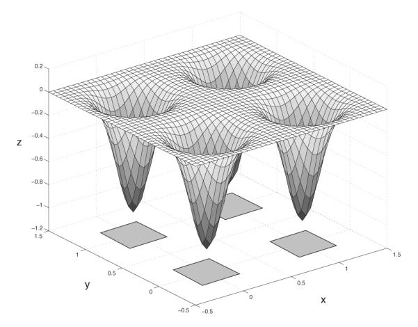
Four potential wells, implementing four symbols in the (x, y) state space of two units’ activations.
As a reminder, the analog state space (or phase space) of the system we will examine consists of vectors of real numbers, each greater than or equal to 0 and less than or equal to 1. When we are faced with more than two phase space dimensions (i.e., more than two units), the energy surface is difficult to depict graphically. Nevertheless, the analog state is equivalent to a point moving inside a hypercube (i.e., a ‘brain state in a box’, in the colorful description of Anderson et al., 1977). Each dimension corresponds to one unit in the system, and an energy surface can still be well-defined.
Since we assume the presence of noise, the non-overlapping regions of state space must be separated by a no-man’s-land that is not associated with any state. Otherwise, a stochastic process involving white noise perturbations that is leaving one region and entering another is likely to make multiple, back-and-forth crossings of a region-boundary during a single intended FSA transition. A separated analog state region is consistent with the TTL voltage band convention. Fig. 5 shows regions in the x − y plane that denote four distinct symbols, separated by large regions that do not encode any particular state of an emulated four-state FSA.
4.2. Threshold mechanisms
Since the behavior of an emulated FSA will be conditioned on the entry of an analog state into a symbol region, threshold-crossing detection will be an essential function of our system (as it is in any computer). Mathematically, it is easy to define a quantity (an indicator variable) that specifies whether the analog state of a system is within a symbol region, such as the TTL regions for 0 and 1 in digital systems. An indicator variable for a single voltage takes on the value 1 when a voltage is inside a region, and 0 when it is outside, making it a step function — or Heaviside function — of the analog state variable.
4.2.1. McCulloch-Pitts neurons
In general, approximations to step functions will play critical roles in our models in determining whether or not to make a response. However, using step functions per se would present serious difficulties for the type of model that we address in section 6. Ultimately, we will derive instead a simple mechanism for approximating a step function with arbitrary precision using only the leaky integrator units we presented in section 2. First, though, we state the definition of McCulloch-Pitts neurons (McCulloch and Pitts, 1943) explicitly in Eq. 14, and we analyze the problems this model presents, especially when the discrete time steps (n) are generalized to continuous time (t).
Formally, the activation Vi of the ith unit in a system of McCulloch-Pitts neurons in response to input Ii is as follows:
| (13) |
| (14) |
Eq. 14 is very similar to Eq. 3 in that it computes a weighted sum of its inputs. The effective threshold can be increased or decreased from Θ by providing a constant input (or bias) to the unit. A positive bias in effect shifts the function to the left (decreasing the threshold), and a negative bias shifts it to the right (increasing the threshold). A simple but effective technique for adapting response thresholds (and speed-accuracy tradeoffs) to changing task conditions derives from this fact (Simen et al., 2006).
However, there are critical problems with this idealized approach to thresholds regarding its physical and biological plausibility. Furthermore, a disastrous, noise-induced ‘chatter’ effect is easily produced by artificial mechanisms that approximate these idealized thresholds. Without compensating mechanisms, thermostats that use temperature readings to govern a furnace, for example, can rapidly switch a burner on and off as a room’s temperature hovers noisily around the thermostat’s temperature threshold, thereby wasting energy and possibly damaging the furnace.
For our purposes, the worst problem with McCulloch-Pitts units is that, by themselves, they cannot maintain an encoded FSA state in the interim between received state-transition signals. Therefore, we either need to guarantee that the intervals between input signals to the FSA are shorter than the decay time of our state-maintaining units (an unnecessarily strong constraint), or we need to ensure that state can be encoded indefinitely (or latched) as is done in digital electronics. Latching is the path we will take.
We achieve latching and avoid the chatter problem with the use of strong, recurrent self-excitation in ‘readout’ units, like those in the second layer of Fig. 4. This results in bistable dynamical systems with exactly two equilibrium points that produce all-or-none behavior of the desired type. Bistability will play an important role in our proposed architecture, as it does in other neural modeling approaches and in digital electronic circuit components (Hayes, 1993). Bistable striatal neurons in mammals, for example, are thought to produce action initiation by promoting signal propagation through the basal ganglia (Alexander et al., 1986). Because of its role in action initiation and sequencing (Aldridge and Berridge, 1998), the most recent version of ACT-R has associated production firing with the basal ganglia in its mapping from the architecture onto the brain (Anderson et al., 2004). We proposed a similar mapping in Simen et al. (2004).
Thus recurrent excitation defines the symbolic/subsymbolic interface in our approach to cognitive modeling, by turning a nearly linear system into a highly nonlinear (nearly binary) one.
4.2.2. Hysteresis
In general, bistability and latching are properties of many systems that display hysteresis: that is, systems whose outputs do not depend exclusively on their immediate inputs, but also on the recent history of the system’s outputs. Fig. 6 shows a classic example of a bistable system with hysteresis. The vertical axis represents output values, and the horizontal axis represents input values. The solid curves denote stable equilibrium output values as two, distinct functions of the input values. The dashed curve represents unstable outputs as a function of inputs: for any coordinate pair that lies on this curve, any perturbation of the output will cause it either to increase to the upper solid curve segment or to decrease to the lower solid curve. The resulting dynamics of such a system are that upward velocities occur as the input increases above point A if the output starts out on the lower solid curve (these velocities become large as the input grows greater than A). Similarly, downward velocities occur as the input decreases below B if the output starts out on the upper solid curve. For any input I in the range between B and A, the system’s output value has either the lower or upper solid curve as its equilibrium, depending on whether the previous output values were, respectively, below or above the dashed curve.
Figure 6.
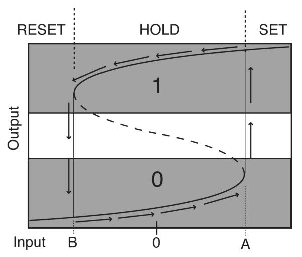
A latch based on hysteresis. The solid curves denote stable, attracting points: for any given, constant level of input, I, the system will eventually converge to a point on one of these curves centered above I on the horizontal axis. Where a dashed curve is plotted, two possible attractors exist for the same input value. Which curve the system converges to (assuming I is held fixed) is determined by the current output value of the system: if it is above the dashed curve, it will converge to the upper solid curve, otherwise to the lower curve. If the system starts out on the solid curve in the lower left corner of the diagram, and input increases, it will follow the trajectory denoted by the arrows. Input value A then defines a threshold for inputs that drive the system to a high level of output activation (corresponding to a binary 1). If inputs then drop below A, the system retains nearly maximal activation until input drops below the value B, at which point output will plunge to the lower attractor (a binary 0). It can store a 1 or a 0 as long as the input is between A and B, and will be least susceptible to noise at the midpoint between them.
Hysteresis has historically been employed for a variety of functions in psychological and neural models, including shortterm memory (Cragg and Temperley, 1955; Harth et al., 1970; Nakahara and Doya, 1998), abrupt changes in conditioning and extinction (Frey and Sears, 1978), and critically, the implementation of population thresholds for activity that are robust to noise (Wilson and Cowan, 1972). A simple method for controlling the amount of hysteresis in the bistable units we propose for threshold-crossing detectors will be the principal technique that allows us to construct models capable of complex, sequential processing. Also, while we have noted that the vertical translations in the hysteresis diagram in Fig. 6 can be rapid, circuits with cyclic connection patterns (as discussed below) will sometimes require in addition a method for controlling the speed of the vertical translations. In fact, for inputs only slightly greater than A, the upward vertical velocity is very small for solutions that are leaving the lower, stable equilibrium curve, so that input strengths can be tuned to achieve arbitrarily slow translations in the absence of noise.
We now show how input latching and resetting can be achieved if we can assume that our units display hysteresis. Rather than using an ‘enable’ line, as in typical electronic latches, this latch operates more like a static RAM cell in computer memory: it loads a new value when forced with a strong input that overwrites its currently stored value. Here, ‘strong’ inputs are those that are greater than A or less than B. As we show below, we can parameterize our units so that input signals of strength near 0 occur at the midpoint of the unstable (dashed) curve, as in Fig. 6. When strongly positive inputs greater than A are received for a duration long enough to drive the output into the 1 region, the latch is ‘set’, independently of the previously stored value. When strongly negative values (less than B) are received for long enough to drive the output into the 0 region, the latch is ‘reset’, again independently of the previously stored value. When inputs in the intermediate range are received, they change the output value slightly, but they are incapable of driving the output out of the symbol region for the currently stored symbol.
4.2.3. Threshold-crossing detectors and latches built from self-exciting, sigmoidal, low-pass filter units
Positive feedback in sigmoidal units is the key to generating the hysteresis properties that we need for threshold-crossing detection and latching, just as it was the key to achieving a larger time constant for linear units in section 2. We therefore consider the dynamics of a self-exciting unit, whose output value V is weighted by a nonzero synaptic strength w and added to the weighted sum of its other inputs. A standard result for such units is that supplying them with positive feedback is mathematically equivalent to changing the shape of their activation functions. We can achieve latching in this way, and we can also achieve precise control over the speed of this latching. Control over this aspect of hysteresis is what will allow us to connect units into network topologies containing small cycles, which in turn will allow us to build concurrently operating, self-timing circuit components with ease.
We can determine the effects of recurrent excitation by two methods: the first is the hysteresis diagram that we have already discussed, which will allow us to interpret self-excitation as a deformation of a unit’s activation function; the second method, based on ‘cobweb diagrams’ (Jordan and Smith, 1999), is covered in the supplementary materials. The latter technique is extremely useful for model construction, allowing the designer of a model to estimate the rate of change in activation at a given pair of input and output values by visual inspection. This method in turn supports an efficient procedure for setting the connection strengths between units in large networks so that desired behaviors are achieved. However, the workings of architecture components can be understood without delving deeply into the details of this technique.
Diagrams like those in Fig. 6 are sufficient for this purpose. These figures can be computed by numerically finding the points in the input-output plane at which the derivative dV/dt in Eq. 3 is equal to 0, using Newton’s method, for example. (The utility of cobweb diagrams is that they do not require this computationally expensive step.) The activation derivative can also be computed at a grid of points in the input-output plane, so that nonzero velocity vectors can be plotted (with arrowlength proportional to magnitude) to give a global picture of how the system changes as a function of position. The plots in Fig. 7 show this approach: a system with self-excitation that perfectly balances its leak is plotted on the left (we will refer to such units as balanced); a system with stronger self-excitation results in bistability and is plotted on the right (we will refer to such units as strongly self-exciting); units with weaker self-excitation (not shown) will be referred to as weakly self-exciting (a weakly self-exciting unit’s activation function will look more like the non-self-exciting activation function shown in Fig. 2E; weak self-exciters act as leaky integrators with an adjustable time constant that increases as the recurrent weight increases, as in Eq. 20).
Figure 7.
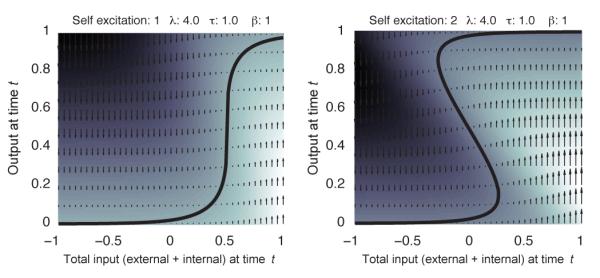
Phase plots for units with balanced (left) and strong (right) recurrent connections to themselves. Here equilibrium curves are plotted as solid curves, and velocities are plotted by arrows and shading (white corresponds to positive, black to negative velocities).
A unit’s activation function can also be computed over a range of self-excitation strengths and plotted as a surface. Fig. 8 illustrates this graphical approach. This type of diagram is a depiction of a ‘cusp catastrophe’ (Thom, 1989), in which a particular type of sudden, ‘catastrophic’ change occurs in the shape of the equilibrium curve (which in our case is an activation function) as some parameter of the system changes continuously (in this case, the strength of self-excitation). The equilibrium curves in the bottom plots of Fig. 7 are equivalent to vertical slices through this surface that run parallel to the Input axis. The catastrophic change that occurs as recurrent weight strength increases is the sudden appearance of three equilibrium points for certain input levels (and therefore hysteresis too), whereas for smaller recurrent weights, there is only one equilibrium point (and no hysteresis). The so-called ‘bifurcation’ value of self-excitation at which this change occurs happens to be equal to the slope of the original sigmoid activation function at its inflection point, as shown in the supplementary materials. At this special value (i.e., when it is balanced), the system approximates a perfect (non-leaky) integrator. We discuss an interval timer in section 6 that exploits these dynamics in order to time out unsuccessful steps of computation and generate subgoals for problem solving.
Figure 8.
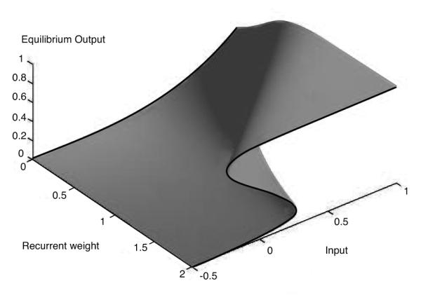
Effective activation functions for a range of self-excitatory, recurrent connection strengths, plotted as a ‘catastrophe manifold’. This system produces a cusp catastrophe as self-excitation increases above 1 (in general, such catastrophes occur when self-excitation increases above λ/4, where λ is the maximum slope of the sigmoid activation function (i.e., the activation function for self-excitation equal to 0). Given a particular recurrent self-excitation strength, w, a vertical slice through this surface parallel to the Input axis and positioned at w on the Recurrent Strength axis gives the effective activation function for that value of w.
4.2.4. The closed-loop problem
The primary self-timing operation that independent, concurrent processes in our model will invoke once activated is to prevent other processes from interfering with them until they have finished their work (if possible). This includes preventing new inputs to a process from being accepted once the process begins. It also includes waiting for indications that the result of a process has been computed, and then cancelling itself. Both of these types of handshake operation can be achieved with cyclic connection patterns involving excitation and inhibition (Sparso and Furber, 2002).
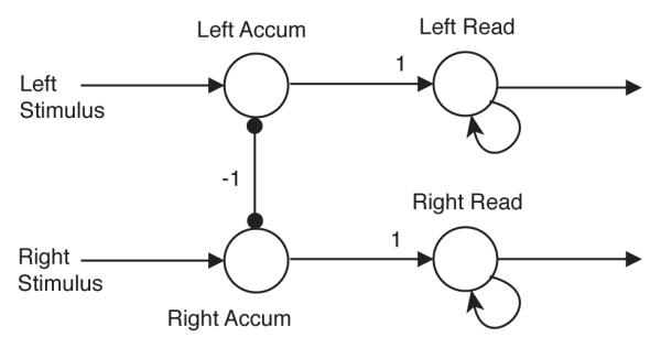
Here we examine the simplest example of such a system, depicted in Fig. 9: two units, IN and OUT, in which IN excites OUT, which in turn inhibits IN. Once IN is inactive and OUT is active, we might want OUT to persist in its activity indefinitely, or to persist until being inhibited by some other unit (not depicted), or finally to return to inactivity after a delay of controllable duration. We now address parameterizations and a technique for finding them that allow these behaviors to be realized.
Figure 9.

Three different parameterizations of a two-unit closed-loop system intended to propagate a 1 forever (from the OUT unit) and to wipe out input layer activity (in the unit IN) once the first input pulse is detected. Activation over time is shown for each unit in the top two rows of each subfigure. The input signal is shown in the bottom row. A: Feedforward and feedback connection strengths between IN and OUT are too weak to cause propagation of the input pulses; B: Interconnection strengths suffice for the desired behavior; C: Interconnection strengths are too strong, once again causing failure of input pulse propagation.
Fig. 9 shows the activation levels of the two units over time, under three different parameterizations, in response to two step pulses of input of amplitude 1. The only parameter that varies in the three sets of plots is the strength of the connections between IN and OUT. The intended behavior of the system is to detect the first input pulse, thereafter propagating a 1 from OUT and making IN unreceptive to external inputs. Both units are parameterized with bias β equal to 1.2, gain λ equal to 4, and recurrent excitatory connection strength 2. Each subfigure of Fig. 9 shows the timecourse of activation in a two unit network receiving a pulsed input. The top two graphs of each subfigure show the activation of the unit illustrated next to the graph. Subfigure A and C both show failures to achieve the intended behavior due to interconnection strengths that are too weak and too strong, respectively. Subfigure B shows the intended behavior being executed.
4.3. Elementary logic functions
Using hysteresis diagrams, we now demonstrate that self-exciting, nonlinear leaky integrator units can implement a complete set of logic functions (a set, like {AND, NOT}, that can be used to compute any propositional logic function). We will then have the means to compute the state-transition table for any FSA.
Consider a system of two upstream units, A and B, and one downstream unit C, with feedforward excitation from A and B to C, as in Fig. 10. In order for C to respond as the neural equivalent of an AND gate in digital logic, the following behavior is required: when A and B are both highly active, C should be highly active. If either A or B are inactive, C should be inactive. C should never linger at values that are far from 0 or far from 1.
Figure 10.
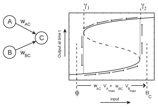
Parameterization for an AND gate, C.
The following parameterizations, illustrated in Fig. 10, give this behavior. C should be strongly self-exciting, and θC should be greater than γ2, the bifurcation point at which two stable equilibria and one unstable equilibrium collapse to a single stable equilibrium. The connection strengths from A and B to C should sum to a value sufficient to exceed this threshold when added to the baseline level of input to C (in Fig. 10, this level is a point ϕ to the left of γ1). Thus when A and B are highly active, C’s effective activation curve will have a single equilibrium value near the maximum possible output value of 1. Without a drop in A or B, C will eventually become highly active. The time that C takes to become active will depend on how far to the right of γ2 is the weighted sum of C’s inputs, because this horizontal position determines the size of the upward velocity vectors (shown in Fig. 7). For horizontal coordinates arbitrarily close to, and greater than, γ2, the diminishing upward velocity vector length indicates that C’s ramp-up time will be arbitrarily long. (Strictly speaking, the time to approach an attractor is always infinite, since attractors are approached exponentially. By ‘ramp-up time’ we refer instead to the time required to approach within some nonzero-diameter neighborhood of an attractor, which happens in finite time.) Thus, faster decision making requires the sum of input from A and B to exceed γ2 by a larger amount (that is, to excite C more strongly).
With strong A → C and B → C connections (denoted wCA and wCB respectively), however, there is the potential problem that strong activation in only one of A or B will be sufficient to activate C. In order for C to retain the property of being a conjunction detector, the connection strength from each of A and B to C must be less than θC − γ1. Thus a requirement for faster conjunction detection requires both that θC be larger and that the feedforward connection strengths be larger and roughly equal, each less than θC − ϕ, and with sum greater than θC − ϕ.
Finally, we note that the connection strengths used in–this discussion are approximations. The units A and B in this example will never quite reach an activation of 1 or 0. Weights and θ’s must therefore be set with a margin for error that is discovered through trial and error when building a system (in our experience, this is quite easy to do).
We have shown the parameterization of a three-unit network that computes an AND function. We omit the description of OR and NOT functions; interconnection strengths that compute these functions are straightforward modifications of the values depicted in Fig. 10.
4.4. Using attractors in the form of latches to maintain state
We now address the means by which the proposed system can maintain the representation of an FSA state in between the reception of transition-triggering signals, and the means by which signals can trigger transitions from one FSA state into another.
We do this by parameterizing the strength of a connection from the old state-encoding unit (or units) to the new state-encoding unit(s) — and from the input to the new state-encoding unit — so that together, the old state plus the new input cause activation of the new state. That is, each state-encoding unit acts as an AND gate that detects the conjunction of the old state and the new input, and whose hysteresis properties maintain the new state after the input disappears, even in the presence of noise. In this way, state can be maintained with high probability and for long durations in between signals (although noise will eventually produce an escape from the potential well defining a state with probability 1 — see Gardiner, 2004 — implying a practical limit on working memory duration).
4.5. Using flip-flops to prevent critical race conditions
There is a well-known problem with using latches to maintain state that has been solved in digital logic design with the use of flip-flops (Hayes, 1993). The problem is that computations often need to use the maintained state in order to compute the next state. If state is maintained by latches, then the old state can begin to be overwritten by a new internal signal even as that signal is being computed. This can easily result in a failure to complete the computation of the next state. In that case, the result is an unpredictable state, or a rapid oscillation between 1 and 0 known as a ‘critical race’ condition, or even metastability: persistence in a state in the analog state space that is not within any of the symbol regions.
To handle these problems, flip-flops are used in digital logic to ensure that only one transition is possible before some additional control signal is received on an enable line, usually from a central clock. Flip-flops maintain two copies of a bit value: the current bit value, and a new value that will become current when the next control signal is received. Rules can be applied to transform old values into new values, but without overwriting the old values until the next control signal. This eliminates any possibility that in the process of computing a new value, the old value becomes destabilized before the computation of the new value is complete. The use of clocked flip-flops is the defining feature of synchronous digital circuit design, and it heavily influences the discrete time-cycle view embodied in most production systems and AI models.
Because we cannot assume a central clock, however, we make each concurrent process determine for itself whether or not to accept input. The method we have used to handle this issue is to cause one or more units involved in a process to strongly inhibit all of that process’s input units once the process has begun, as in our closed-loop example. When reduced to near-0 activation, the input units can neither excite nor inhibit the units carrying out the process. Thus, no input will be accepted by a process until it detects that its processing is complete, or until it decides that too much time has gone by (we discuss the latter in section 6). Nevertheless, we can still make use of locally clocked flip-flops to solve problems involved in generating subgoals during problem solving, as we discuss in the supplementary materials.
To achieve flip-flop behavior, we define a gate to be a copy of an upstream latch component, with one-to-one feedforward connections from upstream units to their corresponding downstream units.4 A second set of inputs to the gate component is strongly inhibitory and reduces all activity in the gate to baseline when propagation of outputs is not desired. The purpose of a gate is to prevent propagation of a latch’s contents without wiping out its activation-based memory. We note that while neural latches are analogous to latches in digital systems, gates as we have defined them are distinctly different than digital components with the same name (AND, NAND, OR gates, etc.). We use this term for our neural component because it is a common term for mechanisms with the same function in the cognitive neuroscience literature (e.g. Frank et al., 2001; Braver and Cohen, 2000).
We have now described the operations of decision making under uncertainty, thresholding, computing logic functions and maintaining state, and we have proposed neural network mechanisms to implement them. These operations give us sufficient computational power to emulate any FSA (and if we allowed ourselves infinitely many filter units, we could emulate any Turing machine with an infinitely long tape — see Simen et al., 2003). The mechanisms are simple: self-exciting, bistable units maintain binary representations of state for arbitrary durations; connection strengths between units and the bias parameters within units determine the logical function that a unit computes on its binary inputs (thereby implementing an FSA’s statetransition table); finally, the bistability of these units leads to approximately punctate transitions into the next state. Aside from the absence of a central clock (which we can achieve by the use of asynchronous timing methods based on closed-loop circuit connections; cf. Sutherland and Ebergen, 2002, and Sparso and Furber, 2002), the result is a network mechanism that is not all that different from a standard, digital electronic circuit, in which units play the role of capacitors and transistors, and connections play the role of resistors. Neural automata of this type can then be used to control a hierarchy of truly subsymbolic processing, as might be carried out in hybrid neural-symbolic models of motor control in animals and robots (e.g. Ritter et al., 2007).
Our discussion of logic-level mechanisms is not yet complete though. We must now consider how decisions are made in the presence of processing conflict — an operating condition described below that typifies the operation of parallel-processing systems such as production systems, but a condition that is purposely precluded by standard sequential-circuit design techniques in digital electronics in order to ensure predictable operation (Hayes, 1993). Since the brain appears to be a parallel processing device, conflict constitutes a central concept in cognitive neuroscience (Botvinick et al., 2001). Aside from the capacity for subsymbolic decision making, it is the presence of processing conflict and mechanisms for resolving it that most distinguish our proposed architecture from standard digital computing techniques.
5. Voting processes that implement if-then rules
Production systems5 (e.g., Anderson and Lebiere, 1998; Just and Carpenter, 1992; Laird et al., 1987; Kieras and Meyer, 1997) are used widely in cognitive psychology and AI to model cognition. These systems exhibit flexibility in their operation relative to standard computer programs, because they decompose the potentially long, complex routines of a standard program into sequences of smaller instructions – if-then rules, or ‘productions’ – which can be conditioned on the state of the world and on current goals, and which can be executed in parallel. Thus production systems are able to sample the world frequently, detect and handle errors quickly, and interrupt long routines if necessary. They are also amenable to powerful learning strategies such as ‘chunking’ (Anderson and Lebiere, 1998; Laird et al., 1986; Miller, 1956) that compile successful rule-sequences into single rules, thereby speeding performance, as well as stochastic, exploratory rule-creation processes in some systems (Holland, 1986a).
Production systems consist of a working memory (WM) for symbolic information (whose contents are typically updated frequently), and a long-term memory of productions (whose contents typically endure for much longer durations). The typical processing scheme for such a system is that the conditions of the production rules are repeatedly matched against the contents of WM. Any rule whose conditions are satisfied becomes a candidate to make the changes to WM specified by its postcondition. These rules are said to ‘match’. Conflict resolution processes that vary among production system architectures may then determine which rules actually execute their postconditions, or ‘fire’. These changes typically occur at the onset of the next processing cycle and do not produce matches of other rules on the current cycle. In Soar, many productions can fire in parallel and generate preferences about the next sequential step to take in problem solving. A separate decision cycle then consults the preferences and commits to a specific mental operator (Laird and Congdon, 2006). ACT-R instead allows only one production at a time to fire (Anderson et al., 2004).
In order to implement production systems in neural networks, the mechanisms underlying this cyclical process must be addressed (or the cyclical model must be modified) in order to observe a constraint that we and others have hypothesized: this is that the brain lacks a global, synchronizing clock circuit. Furthermore, a means must be addressed by which circuits can make decisions about which rules to fire when there is processing conflict between multiple matching rules.
This section addresses both issues in the same manner as Polk et al. (2002). It emulates ‘matching’ by a voting process among competing candidate rules (cf. Grossberg, 1980b; Feldman and Ballard, 1982). This voting is implemented as a high-dimensional diffusion process in a competitive attractor network (or ‘module’), driven by connection strengths that implement preferences among candidates and that connect modules together (cf. the similar feedforward network approach, or ‘Core Method’, for encoding propositional logic statements in Bader et al., 2007). It emulates ‘firing’ as a threshold-crossing event, implemented by strongly self-excitatory neural network units that can operate without governance by global clock signals.
5.1. Production implementations: if-then rules and conflict
We characterized the operation of n-dimensional attractor networks in response to a vector of n constant inputs in section 3. We are now ready to take our most significant step toward the implementation of production systems, by implementing working memory symbols and symbolic productions that may conflict with each other, as was done in Polk et al. (2002). To do so, we consider a simple example of the type of productions necessary for performing the Tower of London task (Shallice, 1982).
This task is depicted in Fig. 11. In it, a participant is shown a starting configuration and a goal configuration of colored balls on pegs; the participant is then asked to transform the starting configuration into the goal configuration by moving one ball at a time. The TOL task has been used extensively to assess planning impairments and is thought to depend crucially on goal management (Shallice, 1982). It is a variant of the Tower of Hanoi problem (Simon, 1975), but in contrast to that task, there are no constraints specifying which balls can be placed on which others. Instead, the pegs differ in how many balls they can hold at one time (the first peg can hold one ball, the second peg can hold two, and the third peg can hold three). There is typically one red, one green and one blue ball. Participants are usually asked to try to figure out how to achieve the goal in the minimum number of moves and are sometimes asked to plan out the entire sequence of moves before they begin (Carlin et al., 2000; Shallice, 1982; Ward and Allport, 1997).
Figure 11.
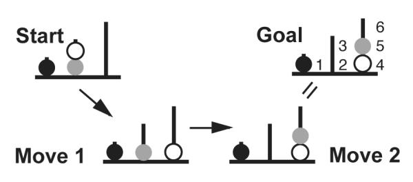
The Tower of London task. Here we have arbitrarily numbered the possible goal positions for easier reference.
In the model discussed in Polk et al. (2002), the representation of the current task state consists of the following symbolic attributes (among others): six numbered gameboard position attributes, each of which can take on one of the four possible color values — blue, green, red, and empty — indicating the color of the ball that currently occupies that position; and a move/action symbol, with eighteen possible values corresponding to every possible conjunction of a ball to be moved and a target position for it to occupy. (Here we rely on a conjunctive code for binding ball colors to positions; a dynamic binding mechanism, which we do not model in this paper, could presumably use fewer units to represent the same thing.) Given the right vector of inputs, we can cause any of these attractor modules to converge to the desired values so that any combination of attribute/value pairs can be represented.
Now we address the general interconnection pattern between modular networks that allows us to produce these constant input vectors. Before considering the production implementation in full generality, we begin with a simple example. Consider the set of two productions in Table 1, which use a Soar-style preference encoding.
Table 1.
A simple set of productions.
| 1) IF (Position2 = Red) THEN (Move = Red-4) Preference = 1 |
| 2) IF (Position1 = Green) THEN (Move = Green-4) Preference = 0.5 |
In this system, the current state of the gameboard determines which rules match. To implement the two productions, we use three attractor modules: Position1 and Position2, representing the antecedent conditions of the production, and Move, representing the consequent of the production. Each Position module uses four pairs of units for representing four possible ball colors, each pair consisting of an accumulator feeding into a threshold unit. The Move module consists of eighteen accumulator/threshold pairs for representing moves. We depict connections among the units of interest in these modules in Fig. 12 (the full model is depicted in the Supplementary Materials).
Figure 12.
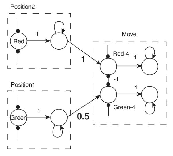
A simple example of a network implementing two productions. We show only the units of interest within each module (there are three additional pairs of units in each of the six total Position modules, and sixteen additional Move pairs in the Move module).
The weights in Fig. 12 define a net input vector in the two-dimensional space of the two Move accumulator units shown. Such vectors are depicted in Fig. 13. Any preference vector in which the elements are not equal will ultimately drive the attractor network into one symbol region or the other (assuming properly parameterized thresholds and bias terms — how to achieve such parameterizations through feedback control is the subject of appendix C). We therefore partition the input space into two half-plane regions by the diagonal line running through the origin and the point (1,1). If no noise is present in the system, the network will deterministically enter the symbol region in the same half-plane as the input vector. If noise is greater than 0, then the probability of entering the symbol region in the same half-plane is greater than that of entering the other symbol region, but it is less than 1.
Figure 13.
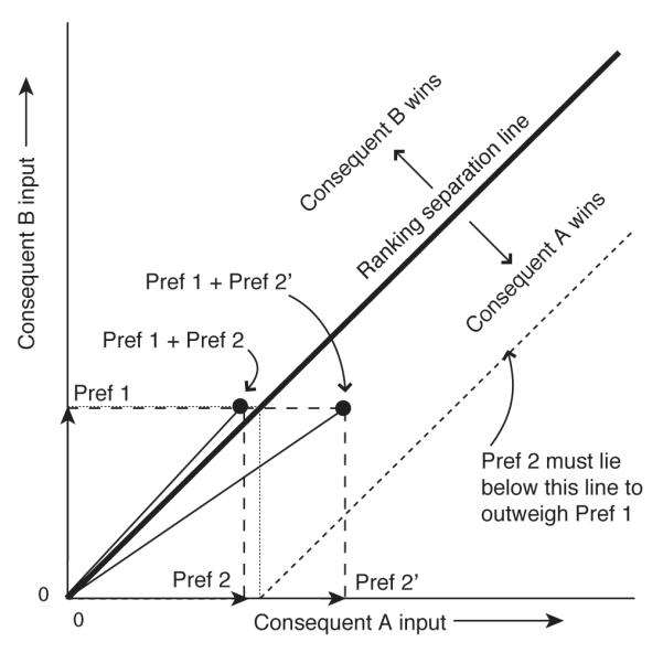
A simple example of three individual preference ratings (arrow-head vectors) specified explicitly by productions, and two combinations of emergent (implicitly specified) preferences (circle-head vectors). Ratings are transformed in continuous time into rankings by the competitive dynamics of the consequent attractor network. Thresholds on consequent unit activity are then used to select a unique winner based on these rankings. Without noise, the highest ranked candidate always wins. When noise is present, a distribution of winners and of decision times results in which the expected choice proportions are ranked in order of the preference ranking.
We can continue in the following way to translate productions into neural networks more generally: create an attractor network for every antecedent attribute that appears in a rule, with one unit in the network devoted to each value that that attribute can take on. Then create weights from those networks to networks that similarly encode the consequents of each rule, with values equal to the specified preference strengths.
Specifically, for the case of n antecedent units projecting in a one-to-one pattern to n consequent units (see the five-unit example in Fig. 19), set the preference ratings Pi, (i = 1 … n) as follows. (For simplicity, we assume that the antecedents are binary-valued.) Pick a base strength B and a difference value, Δ, such that P1 = B, P2 = B + Δ, … Pn = B + (n − 1)Δ. The difference value Δ between preferences should be large enough to guarantee a desired minimum level of expected accuracy in choosing the most preferred option, as well as a desired maximum response time.
While reaction time distributions and expected accuracies are quantities that are given by an explicit formula in the case of the drift-diffusion model of two-alternative decision making (which properly parameterized neural networks approximate), they can only be computed numerically by solving partial differential equations or by Monte Carlo simulations in the case of decision making among three or more options (McMillen and Holmes, 2006). In programming the model of Tower of London performance in Polk et al. (2002), we used a process of trial and error to set B and Δ manually (a task which was made easier by the use of the feedback control methods discussed in appendix C).
5.2. Preference blending
While we do not currently have an automated procedure for setting (or learning) these values, a formal statement of the preference-encoding scheme used by the proposed rule implementation may be helpful for future work on this problem. Let the outputs of the antecedent threshold units be the vector A (whose ith element is Ai), the outputs of the consequent accumulator units be labeled Ci, and the uniform lateral inhibition between consequent accumulators be ξ (we assume uniformity only for simplifying our discussion). Assuming binary-valued outputs from the antecedent units, the net input, Ii to consequent unit i is given by Eq. 15:
| (15) |
Given the nonlinear activation functions of all units (Eq. 2), which prevents outputs from going negative, we can assume that Ci is effectively zero whenever Ai is zero. Thus, whenever any term Aj, j ≠ i, is zero in Eq. 15, no competitive influence is exerted by consequent unit j on consequent unit i. In this way, if antecedent unit j is inactive, then option i can become the most preferred option, even if the connection strength feeding into consequent unit i is smaller than that feeding into consequent unit j.
This picture becomes more complicated when one-to-one connections are generalized to many-to-one and many-to-many connections. In such a case, we must work with a matrix W (whose ith row is labeled Wi) that encodes the preferences P, as in Eq. 16 (which is identical to Eq. 13 apart from changed variable names):
| (16) |
As it happens, most of the interesting action-selection functionality of the Tower of London model in Polk et al. (2002) and in the supplementary materials involves many-to-many connections. Unfortunately, such connections create a serious difficulty for the straightforward mapping of production preferences onto weights that we have described up to this point. The most obvious use of preferences in such a system is to list all matching productions in order of the static preference values attached to them, and then to choose the most preferred. In our system, in contrast, preferences change depending on which rules are matching (they blend together in the form of a weighted sum). We address this problem in the context of fully general preference implementation in appendix D, keeping in mind that what we ultimately want is a means by which any desired preference ranking among alternatives, in response to any current state of working memory, can be imposed by a programmer or learned by a learning algorithm.
6. Models of complex cognition: problem solving
The preceding sections described architecture components that make sequences of decisions and implement if-then rules in a process analogous to holding an election. This is the most important step in implementing production systems. Still, several other high-level architectural features of production systems are required before models built from these components can achieve the functionality of systems like Soar and ACT-R. Principal among them is the capacity to make actions contingent both upon immediate states of the environment, and upon internally maintained representations such as goals and subgoals (Newell, 1990).
Goals and subgoals in our system are represented in the same way as any other symbolic information, using recurrent latch mechanisms. For simplicity’s sake, actions too are represented as the symbolic outcomes of if-then decision processes. Goals exert their influence on these decision-making processes by favoring the outcomes that would help achieve a given goal, using direct, excitatory connections to the units representing those outcomes. This idea is quite simple, and is prevalent in cognitive neuroscience models of related phenomena such as attention (Miller and Cohen, 2001; Desimone and Duncan, 1995; Cohen et al., 1990). This approach to goal implementation leads directly to predictions about the cognitive and behavioral effects of brain damage and disease.
In Polk et al. (2002), we discussed the use of goal and subgoal representations in the context of a model of the Tower of London task. In Polk et al. (2002) and in Simen et al. (2004), we discussed the application of different versions of this model to behavioral data from human task participants, including participants with, respectively, prefrontal brain damage and Parkinson’s disease. One virtue of a subsymbolic approach to modeling these tasks is that brain damage and disease can easily be modeled by parameter changes, such as the weakening of connection strengths or elimination of processing units, for which no obvious counterpart exists in purely symbolic approaches. Here we review these results; in the supplementary materials, we cover the detailed structure and operation of the model in Simen et al. (2004) (this model is similar to that of Polk et al., 2002, but it makes use of the sequential processing mechanisms discussed in section 3 to eliminate the latter model’s dependence on symbolic computer code for sequentializing performance).
6.1. Human performance in the Tower of London task
In Fig. 14, we show the basic behavioral results (Owen et al., 1995) that will guide our interpretation of model performance. In this experiment, participants were instructed to plan solutions to problems that varied in the minimum number of moves required for their solution. Once they had decided on a solution, the task required them to indicate the first move that the optimal solution would require. If they made an error (i.e., their first choice was not the first move in an optimal solution trajectory), they chose again.
Figure 14.

Parkinson’s patients display latency impairments (slower planning prior to first move) in the Tower of London task. Increased latency relative to control subjects is shown by patients at two different stages of the disease, with and without medication in the early stage.
In the top row of plots in Fig. 14, the vertical axis represents a measure of response time: the time from problem presentation to first move selection. The horizontal axis represents the number of moves in the optimal solution. In the bottom row of plots, the vertical axis represents a measure of accuracy: the number of first-move selections prior to selecting the optimal first move.
As can be seen in the bottom-left plot in the figure, prefrontal patients clearly demonstrate accuracy impairments in problems requiring 4 or 5 moves, relative to normal control participants (for problems requiring fewer moves, the accuracy differences were statistically insignificant). However, they show little impairment in terms of latency, as the top-left plot shows.
Parkinson’s patients were examined under medicated and unmedicated conditions, and with a range of symptom severities. The top row of plots shows that in all medication and severity conditions, Parkinson’s patients demonstrated latency impairments relative to control participants, and the impairment was more severe for harder problems (problems requiring more moves). The bottom row of plots shows a pattern of accuracy impairments that is less clear cut. Medicated patients with mild Parkinson’s symptoms showed no accuracy impairment relative to controls. Non-medicated patients with mild symptoms showed accuracy impairments in the hardest problems (although an earlier study, Owen et al., 1992, showed no accuracy impairments in this group). Medicated patients with severe symptoms showed definite accuracy impairments (and also did in the earlier study).
By providing one account of this pattern of deficits, we will be able to evaluate the choices we made for modeling brain circuits involved in problem solving at multiple design levels.
6.2. The influence of goals on decision making
We have discussed the use of connection strengths (like those from Perception to Action in Fig. 15) to encode preferences among options in decision making: when the unit assigned to one option is excited more strongly than the unit assigned to another option — because its input connections are stronger, for example — then the first unit is likely to cross threshold before the second. The probability of this event depends on noise levels and connection strengths.
Figure 15.

The basic architectural framework: units in a perceptual network excite and inhibit units in an action-selection network. Units in a goal network bias the competition taking place in the action-selection network.
This probabilistic choice mechanism leads to stochastic exploratory behavior, and preference encodings lead to exploration that is biased toward more-preferred options (Loewenstein and Seung, 2006; Montague and Berns, 2002; Soltani and Wang, 2006; Simen and Cohen, in press). When preferences vary greatly among different options, there is likely to be less exploration and little conflict between options, because the most preferred option will usually win and will usually do so rapidly. When preferences are nearly equal, however, so that many options are equally competitive, a state of prolonged conflict can ensue. To resolve it, thresholds can be set low, resulting in purely exploratory behavior through rapid, random choice; or thresholds can be set high. In the latter case, some other mechanism must instead resolve the resulting, intractable conflict between competing options. Goals are one mechanism that can be used to resolve this type of conflict (we discuss a second, less knowledge-intensive mechanism for conflict resolution based on feedback control in appendix C; this mechanism is essential for preventing critical problems faced by the decision making components of the proposed architecture, but we assume for the present purposes that these problems have been solved).
A serious limitation of the weight-encoded preference approach to choice is that preferences are static in the proposed architecture. Static preferences imply a lack of flexibility in choice that will make effective problem space search impossible. Dynamic wiring is an obvious potential solution to this problem, but it is beyond the scope of this paper. Even in an architecture with dynamic wiring, however, weight-encoded preferences cannot change faster than the weights themselves. For this reason, rapid preference adjustments require rapid weight changes if weights alone mediate preferences. Unfortunately, a large degree of plasticity can be very disruptive to neural networks. This phenomenon is known as a stability-plasticity tradeoff (Grossberg, 1987).
In order to carry out problem space search, however, the choice of an action to take at any given state should be highly context-specific. The current state should certainly help determine what the next move in the problem space should be, and search heuristics might also play some role. Based on its success in explaining many aspects of human problem solving behavior (Newell and Simon, 1972), means-ends analysis is the search algorithm we emulate here (minus that algorithm’s formulation of goals, which is beyond the scope of this paper). Under this algorithm, the most important unachieved aspect of a solution is worked on first, and this work may generate subgoals that must be achieved before the parent goal can be achieved. Therefore — assuming that a current goal is guiding the search — goals must be a part of the context in which actions are selected, and goals should therefore dynamically determine preferences.
We implement dynamic preferences while avoiding the stability-plasticity dilemma and even the need for dynamic wiring by drawing on the idea of activation-based biasing (Miller and Cohen, 2001; Desimone and Duncan, 1995; Cohen et al., 1990). We use a separate network (Goals in Fig. 15) as a context representation that acts to favor a subset of the units within a decision making network. This separate goal network may be capable of representing arbitrarily many contexts. Each context is assigned a strongly self-exciting, approximately binary unit. This unit again uses a suite of static connection strengths to excite units in the decision network and thereby create a temporary preference ordering (one that is in force as long as the context unit is active). In a different context, though, a different context unit becomes active and the previously active context unit inactivates — a process that can happen rapidly. Now the strengths of the new unit’s connections to units in the decision network determine the choice preferences in that network (probably different preferences). However, the previous preference ordering is not lost as a result of connection strength adaptation; instead, the inactive context unit’s connections to units in the decision network maintain the memory of the previous preference ordering for later, rapid retrieval.
The hybrid neural/symbolic Tower of London-solver modeled in Polk et al. (2002) used goal context units in this way to bias the selection of actions in the Tower of London task. In that model, the current state of the game determined which moves were possible (the units representing currently illegal moves, such as moving a ball to a position which is already occupied, were strongly inhibited). The units representing the current state of the game also defined a preference ordering among possible moves, by favoring moves of balls to lower positions on a peg over positions higher on the same peg. This still left multiple options available to the system at many choice points during problem solving. Goal units played their roles at these choice points, guiding the system to select from among a restricted subset of actions by temporarily increasing the preferences for the favored subset (in fact, actions in Polk et al. (2002) and in the model presented in the supplementary materials are restricted to a subset consisting of only the action that would obtain the goal in one move, but this restriction may be loosened).
If goal-unit connections to a decision network are strong enough and noise is weak enough, this guidance can cause nearly deterministic selection of the favored action. However, the key to proper problem-space navigation is to balance the excitation of goal-achieving actions against the inhibition used to prevent illegal moves. Our model relied heavily on such inhibition of the main decision-making network; this was a modeling choice that is consistent with evidence from brain imaging for selective facilitation and suppression by attentional processes of localized, functionally defined brain areas in tasks with conflicts between stimulus dimensions (Polk et al., 2008). When the action that would immediately achieve a goal cannot be chosen because of massive inhibition, the model can either choose some other move randomly, or remain stuck in a problem-solving impasse.
6.3. Normal performance, simulated PFC damage, and simulated Parkinson’s disease
We now review the results of previous simulation studies, showing how a model of Tower of London performance captures the response time and accuracy of typical task participants and of patients with prefrontal damage or Parkinson’s disease. As in Polk et al. (2002), we assume that PFC damage, especially damage to dorsolateral prefrontal cortex (DLPFC), reduces or eliminates the populations of neurons that implement a network devoted specifically to representing subgoals. This assumption is consistent with other modeling work that assigns the DLPFC a role for working memory in problem solving (e.g., Goel et al., 2001), as well as with the behavior of prefrontal patients (Kimberg and Farah, 1993). These patients can frequently carry out basic tasks, but cannot organize sequences of basic behaviors into coherent, complex behavior that achieves goals.
As shown in the left two panels of Fig. 16, prefrontal patients encounter difficulty in achieving an optimal solution to the puzzle (a solution trajectory that involves a minimal number of moves), but only when the required number of moves to solution exceeds three (Shallice, 1982; Owen et al., 1990). The model of Polk et al. (2002) displays a very similar pattern: no more than the optimal number of moves are made when problems require only two moves of a ball. However, when three or more moves are required, the problem typically requires a subgoal: that is, one or more of the balls must not be moved to its final, goal position, even when that position is free, so that the free position can be used temporarily by another ball (ordinarily, so that the order of a stack of balls can be reversed). When our model’s subgoal module has a reduced ability to guide action selection by voting for certain actions and against others, noise leads more often to random selections of a ball. Furthermore, as shown in Fig. 17, base-level goals defined by the final goal configuration of the problem tend to override a reduced subgoal influence in such situations, leading to greedy moves of balls to their final positions. This occurs despite the fact that a lookahead search would have identified that such a move should be inhibited until after a subgoal has been achieved.
Figure 16.
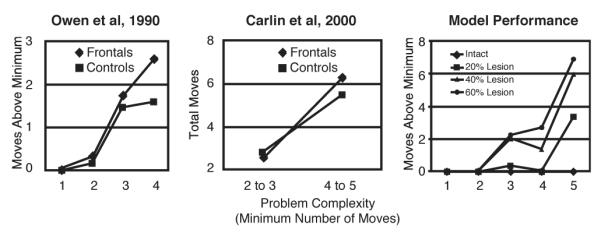
Comparison of the model in Polk et al. (2002) (right panel) to normal and prefrontal performance in the Tower of London task from two studies (left two panels).
Figure 17.
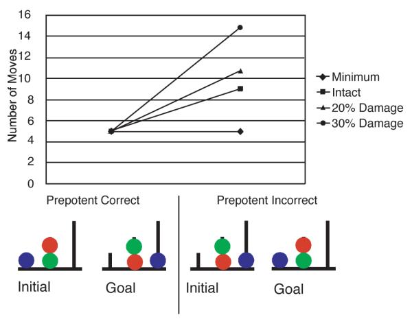
Impaired ability of the prefrontal model to inhibit ‘prepotent’ moves in Polk et al. (2002). Problem solving difficulties in that model stemmed from an inability to prevent moves that achieve component goals when they are legal, but conflict with the current subgoal. The two problems shown involve the same moves, but in the reverse order (initial and goal states are reversed). Damage to the model (i.e., weakening of connections exerting subgoal influence on action selection) leads to disproportionate difficulty with the problem on the right in which prepotent moves must be inhibited.
In severe cases of Parkinson’s disease, the same pattern of deficits is seen; in milder cases, the accuracy of performance is indistinguishable from normal performance. At all levels of Parkinson’s severity, however, impairment in problem solving latency (the time to begin problem solving once a problem has been presented) is seen. Interestingly, however, this impairment appears only on problems requiring more than three moves. A similar latency effect is not seen in prefrontal patients (Owen et al., 1992, 1995).
To simulate the effects of Parkinson’s disease, we weaken the connection strengths that implement propagation delays within an interval timer circuit that is used for impasse detection during problem solving (Simen et al., 2004). Interval timing deficits — specifically, slowing of an internal clock — are a robust phenomenon in cases of Parkinson’s disease (Meck, 1996). The impasse timer in our model, which is discussed in more detail in the supplementary materials, is used to sense when a period of intractable conflict between actions has extended beyond a certain duration. When this occurs, the fully functional model employs a cascade of asynchronous logic circuits (discussed in section 4.3) embodying basic knowledge about block-stacking tasks to compute which subgoal the model should work on in order to make base-level goals achievable. This timer sequentializes problem space search by bottling up activation in an action selection network, and allowing this next step of problem solving to proceed only after the predetermined delay.
Since the timer slows down under simulated Parkinson’s disease, problem solving also slows down in this simulated disease condition — but this slowdown in problem-solving only occurs when subgoals are required. When they are not required, the model proceeds through action selection without any additional bottling up of processing in the action selection network. For this reason, the model only slows down significantly when solving problems require three or more moves, thereby replicating the response latency data in the literature.
The basic functionality of the models discussed here rests on a symbolic representation of task knowledge, goals and actions. However, the basic response time and accuracy predictions of the models depend strongly on manipulations of the subsymbolic substrate supporting this symbolic processing.
7. Discussion
The processing that occurs in a standard computer is highly sequential: most components of the machine are not changing in activity during a processing cycle; only CPU components such as the arithmetic/logic unit and one memory location are typically changing their values on a given clock cycle, but these cycles are incredibly brief and computation is therefore fast nevertheless. In contrast, of course, brains appear to involve a large amount of parallel processing by relatively slow components. Furthermore, while tantalizing hints about timing signals may be perceived in electrophysiological recordings of phase-locked oscillations across widely separated brain areas, the basic technique of computer hardware design in which synchronous digital logic circuits are clocked by a central oscillator seems like a non-starter as a physical model of the brain.
Our approach to these mismatches is to assume as much parallelism as possible, and to push as much computation as is feasible onto a substrate of untimed, asynchronous, neurally implemented voting processes. When conflict between processes competing for neural resources forces a slowdown in processing that would be catastrophic, sequentialization occurs: that is, an agent learns (through a process we have not specified) to implement a set of essential sequence control mechanisms. These include processing bottlenecks (consisting of feedback-regulated decision making components), handshake completion signals, deadline timers and flip-flops for the prevention of critical race conditions. These mechanisms can be straightforwardly applied to the underlying, analog processes commonly used in psychology and neuroscience to model choice and decision making by animals across the phylogenetic spectrum. The result is a system that can be made to approximate basic production system behavior arbitrarily precisely.
The theoretical position staked out by this paper is consistent with the idea that information processing systems can best be understood by decomposing them into mostly independent levels of analysis. That is, systems can be analyzed and understood at one level of analysis while (mostly) ignoring the details at other levels, as in other hierarchical theories of brain function (e.g., Cooper and Shallice, 2000; Eliasmith and Anderson, 2003; Marcus, 2001; Sun et al., 2005). This approach simplifies the task of understanding, because it facilitates the focusing of attention on a smaller part of the overall problem at any given time.
In accordance with this view, we have explicitly followed a levels-of-analysis organizational scheme in the paper. Of course, the notion of total decoupling between levels is idealization that is not likely to bear up under close enough examination. David Marr’s position at the end of his seminal work on vision (Marr, 1982) is consistent with this notion as well:
Question: Are the different levels of explanation really independent? Answer: Not really, though the computational theory of a process is rather independent of the algorithm or implementation levels, since it is determined solely by the information-processing task to be solved. The algorithm depends heavily on the computational theory, of course, but it also depends on the characteristics of the hardware in which it is to be implemented. For instance, biological hardware might support parallel algorithms more readily than serial ones, whereas the reverse is probably true of today’s digital electronic technology.
— David Marr, Vision
Indeed, we have argued that changes at the lowest levels have important impacts at the highest levels. These show up, for example, in simulations of problem-solving performance by patients relative to healthy control participants (Polk et al., 2002). Thus, this paper has relied on a levels-of-analysis organizational structure, but each section of the paper has focused on the interface between two, adjacent levels. In this way, the extent of their independence could best be analyzed. Furthermore, this structure was intended to facilitate understanding of the way in which the effect of a biological or psychological constraint at one level propagates up the level hierarchy. The ultimate result was that low-level changes did indeed have an impact on the way behavioral data could be accounted for by a computational theory at Marr’s uppermost level of analysis. However, though we have argued that this impact was substantial, it was not a complete revolution: the basic notion of problem-space search carried out by a goal-driven system consisting of simple if-then rules is still the simplest way to describe the system we have simulated. We therefore propose the principles embodied by this system as an implementation-level theory that is roughly consistent with much of the computational theory already proposed for explaining complex cognition, most of it symbolic in nature.
Where this paper differs from much of this existing theory, and where it begins to overlap with connectionist and other subsymbolic theories, is in the degree of emphasis it gives to the implementation level. We have further decomposed Marr’s lowest level, that of implementation, into the physical and logic levels in the design-level hierarchy of computer engineering. This decomposition has allowed us to focus on low-level modifications that borrow heavily from neural networks and from analog computation.
We have seen that serious problems remain to be addressed before the principles in this paper can be used to support the whole range of computational-level theorizing that currently takes place using the standard computer as its implementation-level medium. These include the dynamic wiring and binding problems (it is worth noting that previous research groups have attempted to merge production systems and neural networks, only to abandon further efforts in this direction once the difficulty of the binding problem was fully appreciated: e.g., Touretzky and Hinton, 1988; Touretzky, 1990). But, as will be obvious to readers with a background in neuroscience, we have also given short shrift to the physical level, our lowest level of analysis. We have entirely ignored the complex dynamics possible in spiking neural networks in which neurons are governed by the Hodgkin-Huxley equations, or even by simplifications of these equations that are not quite as simple as our RC-filter models of populations.
Ultimately, however, our hope is that the choice of an extremely simple model of neural computation may serve the goal of unifying disparate psychological theories that Allen Newell spelled out in Newell (1990). Some variety of random-walk mechanisms was proposed there as a possible substrate for a complete cognitive architecture. In his words:
Any mechanism with the common properties epitomized in Fig. 1-11 [a diagram of a random walk decision making model] will do all right. This means that we may be able to settle on an important schematic characterization of an elementary mechanism of the mind. And we can trust the incorporation of this mechanism into unified theories of cognition that may appear to have quite different structure.
— Allen Newell, Unified Theories of Cognition
Symbolic and subsymbolic modeling approaches are indeed quite different in structure. But considering these two approaches merely as two different levels of description and focusing on the interface between them highlights the possibility of their ultimate compatibility. In more practical terms, a better understanding of the symbolic/subsymbolic interface may simply help cognitive modelers pick the right tool for a given job.
Supplementary Material
Figure 18.
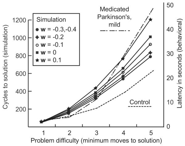
Impaired latency in the current model of Tower of London due to simulated dopamine depletion (modeled as a decreased connection strength, w, that governs the speed of a subgoal-generation timer). Latency must increase supralinearly with increasing problem difficulty since more subgoals in addition to more moves must be generated in harder problems.
A. Filtering out noise by leaky integration
In this appendix, we detail our approach to simulating stochastic integration processes, focusing especially on the central role of leaky integration of noisy signals in our proposed architecture. Leaky integration is a form of sliding window averaging that is equivalent to an exponentially weighted average of a signal y over the infinite past. In discrete time, the weights on the samples of y follow a recursive, difference equation:
| (17) |
As n goes to infinity, these weights sum to 1. For a noisy input signal rn = sn + ∊n, the estimate xn of the signal value sn is then:
| (18) |
Our goal is to minimize the difference between xn and sn — in fact, we will follow common practice and attempt to minimize the square of xn − sn, summed over n.
Furthermore, we will consider a version of this exponential averaging that takes place in continuous time. By doing so, we free ourselves from any dependence on a clock for triggering samples. As the samples come closer and closer together in time,6 and as the weights on individual samples yn are correspondingly reduced at each iteration so that the sum does not blow up,7 the output of the discrete-time signal estimation process (Eq. 18) asymptotically approaches the output of a low-pass RC filter. The differential equation governing the output of such a system in response to a deterministic, non-noisy input signal s(t) is given in Eq. 19:
| (19) |
Here, τ = RC, where R is the resistance and C is the capacitance of an electric circuit implementation, and the voltage V across the capacitor plates is the filter’s output.
Note that with positive feedback through a recurrent connection strength of 0 < k < 1 and with a reduction in input connection strength by a factor of (1 − k), a unit defined by Eq. 19 can achieve effectively any time constant (cf. Seung et al., 2000):
| (20) |
Modeling the effect of a filter applied to a noisy input requires one further complication beyond moving to differential equations: we must use stochastic, rather than deterministic, modeling techniques. For this purpose, we use stochastic differential equations (SDEs), for which a well-developed theory of integration exists (the Ito calculus) (Gardiner, 2004; Oksendal, 2003). The effect of a low-pass filter applied to a noisy input can now be modeled as in Eq. 21:
| (21) |
In this case, s(t) in Eq. 19 is replaced by s(t) + c · dW/dt, where dW/dt is idealized white noise, weighted by a constant,8 c. Strictly speaking, dW/dt is not a well-defined stochastic process in continuous time, although a discrete-time version of dW/dt is quite easy to define and to simulate: dW/dt evaluated at discrete time points n is simply a sequence of samples from a Gaussian distribution centered at 0. Typically, n indexes a sequence of time points spaced apart by some fixed duration Δ. The limiting form of dW/dt as Δ becomes infinitesimal is not well-defined, but the limit of the integral of dW/dt(n) — a Wiener process, denoted by W — is (Oksendal, 2003). A Wiener process, or Brownian motion, is just a continuous-time version of a random walk with steps selected from a normal distribution.
For this reason, we can easily simulate the system9 of Eq. 21 just as we can Eq. 19, using Euler’s method: x(t + Δ) ≈ x(t) + Δ · dx/dt(t). Now, however, at each update of the value of x in a small, discrete time step of size Δ, we also add a normal random variable with mean 0 and standard deviation (Higham, 2001). Obviously then, the way to eliminate any effect of white noise is to make τ large; however, the tradeoff is that a system with τ too large cannot track changes in s rapidly enough.
Of course, the idealized processes of Eqs. 20 and 21 can take on unboundedly large values, but the firing rates of real neural populations are necessarily bounded below by 0 and above by some maximum. Similarly, offset voltages and saturation effects are observed in real amplifiers (Hopfield, 1984; Mead, 1989). Saturation bounds impose a sigmoidal nonlinearity on the output of the RC filter model in Eq. 21 (in applications to brain-modeling, such nonlinearities have been modeled as a logistic function, cf. Cowan, 1967, which is a convention that we too will follow). With sigmoidal nonlinearities in their activation functions, neural network units can be combined to approximate any analog computation conceivable (Cybenko, 1989; Rumelhart et al., 1986).
B. Simplified unit equation
We now derive a simplified, single equation for stochastic unit activity (cf. similar arguments in Brown et al., 2005) from the two-equation systems found in (?). The deterministic part of this equation is identical to standard neural network models, represented by Eqs. 23-23:
| (22) |
and
| (23) |
In general, we will not require the connection strengths, wij between any two units, i and j, to be equal. However, it will simplify matters to assume that the noise coefficients cij on every connection between two units is the same (cij ≡ c), and furthermore that λ and β are the same for all units. (Of course, it might be better to model cij as proportional to f(xj), since neural firing rate variability tends to scale linearly with firing rate; however, the assumption of constant cij may not make a great difference, since f is bounded between 0 and 1.) Assuming that amplification of inputs by all units is instantaneous, we can replace f(xj) with Vj. We then arrive at a single equation for the system, Eq. 24:
| (24) |
If we examine the deterministic part of this equation, and keep in mind Eq. 23, we see that as f−1(V) = x approaches I for some constant input I, V must approach f(I). Furthermore, when x is in the linear range of f, df/dx ≈ λ/4, and f(x) ≈ (λ/4) · x + (2 − λβ)/4. Thus f−1(V) ≈ (4V − 2 + λβ)/4. We therefore get the following deterministic equation:
| (25) |
It is only when V approaches 1 or 0 that nonlinearities affect the approximation, and they will have a small effect. Thus we can use the following, much more manageable equation in our simulations and analyses:
| (26) |
If we assume that λ = 4 (which we can do without any loss of functionality), we can eliminate the df/dx factor to get the simpler equation:
| (27) |
For λ = 4 and β = 0.5, the linearized version of this equation is just the equation for a low-pass RC filter that includes the weighted effects of noise:
| (28) |
Figure 19.

A simple example of five productions. When all five antecedent units are active near 1, then a preference ordering exists: A’, B’, C’, D’, E’. When only B through E is active, the preference ordering becomes B’, C’, D’, E’, A’. Normally, relative preferences are sufficiently large to produce a unique outcome (far right panel), but it is unfortunately quite easy to parameterize a network so that it produces multiple winners (middle panel) or no winners.
C. Integral feedback control of decision making to guarantee the winner-take-all property
In section 3 we discussed the use of lateral inhibition for resolving conflict between multiple, concurrent response processes — a technique that is a principal feature of most neural network-based cognitive models (e.g., Grossberg, 1980a; McClelland and Rumelhart, 1981; Cohen et al., 1990). The dynamics of attractor network convergence in laterally inhibiting, winner-take-all (WTA) networks leads to decisions based on local competition, so that no third party mechanism needs to be invoked, and an infinite regress in identifying the physical locus of deciding and resolving conflict can be avoided. Furthermore, in the case of two competing processes, conflict resolution in linear WTA networks is in fact equivalent (to arbitrarily close approximation) to the SPRT, a statistical decision making algorithm that maximizes earned reward rate in environments with stationary statistics (Bogacz et al., 2006; see section 3).10 Thus, no other conflict resolution mechanism is likely to offer much better performance in such conditions (i.e., more reward per unit time or unit of behavior); nor is any other mechanism likely to be much simpler physically.
As we have noted, though, true linearity is physically implausible, and nonlinear activation functions are essential for the activation hysteresis upon which our architecture depends. Unfortunately, attractor networks of nonlinear filter units often face serious difficulties in selecting a single unit (or a single subgroup of units) for maximal activation. It is all too easy to parameterize a network so that the intended resolution of conflict does not occur, either because multiple competing processes remain active in parallel, or because all of the currently competing processes are silenced (see Fig. 19).
Fig. 20 illustrates this problem in terms, once again, of a phase-plane description of activity in a two-unit decision-making circuit with symmetric lateral inhibition. In section 3, we discussed the phase-plane of a linear system of two units: the activations of the pair correspond to a coordinate pair in the plane, with unit 1 corresponding to the position along the horizontal axis, and unit 2 corresponding to the position along the vertical axis. Starting from the origin of the plane (i.e., both units at 0 activation), the usual idealization of a decision process involves step-like inputs to both units: inputs that instantaneously jump from 0 to some level Ii (Ii > 0, i indexing the units), remaining there until a threshold crossing event, at which time they both return to 0. Usually, I1 is greater or less than I2, and the goal of the process is to determine conclusively which is greater (Gold and Shadlen, 2001).
The picture of such a system in Fig. 2 is complicated by the simplest form of nonlinearity we can impose on the units’ activation functions: a hard lower bound of 0, and a hard upper bound of 1, with linearity in between those extremes. This type of piecewise linearity imposes a bounding box on the system’s activation coordinates. The system must always remain inside this box, depicted with solid lines in Fig. 20. Prior to reaching a boundary, the system evolves like its linear analogue. Once a boundary is reached, however, the system tends to stay there. The boundary is ‘reflecting’ in the terminology of stochastic processes, meaning that the system can in fact hit a boundary and then move back arbitrarily far from it (until another boundary is hit), but the tendency of the system is ultimately to become trapped against the intersection of the decision plane and the side of the bounding box in which the unit with stronger input is most active.
Fig. 20 also shows three different decision planes, whose distance from the origin is determined by the sum of the input strengths (Bogacz et al., 2006). The plane closest to the origin corresponds to weak inputs. It intersects the bounding box at activation values that are below threshold — this is a case of conflict between two responses in which, on average, neither response emerges as the winner. The farthest plane from the origin produces a rapid approach of both units toward maximal activation prior to any disambiguation — this is a case of conflict between two responses that results in both units exceeding threshold within a short time period, on average. If we do not make unrealistic assumptions about instantaneous threshold crossing detection and instantaneous reset of the WTA network to the origin, then this is a case of unresolved conflict with multiple winners that will remain almost equally active and above threshold as long as the input signals are present. Fig. 19 shows an example of unit timecourses in a multiple-winner situation.
Figure 20.
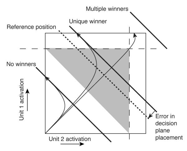
The problems of multiple winners and no winners illustrated in terms of phase planes. Vertical axis represents activation of unit 1, ranging from 0 to 1; horizontal axis represents activation of unit 2, also bounded between 0 and 1. Dashed lines represent thresholds applied to these activations. Exceeding threshold i generates a response of type i. Bold, angled lines represent ‘decision planes’: restricted subspaces which the system approaches rapidly along the main diagonal (shown by three different, curved, arrow-head trajectories). The position of the decision plane depends on network parameterization. When the plane is beyond the thresholds, both units are very likely to exceed their thresholds. When the plane is below both thresholds, neither unit is likely to cross threshold — instead, the system will converge on one of the two intersections of the plane and the bounding box. Feedback control can be used to keep the decision plane in the middle region, in order to ensure a single winner.
One solution to this dilemma that has been proposed is the k-winners-take-all (k-WTA) algorithm that figures prominently in the Leabra system of O’Reilly and colleagues (O’Reilly and Munakata, 2000). This approach involves a mechanism that inhibits all units in the network sufficiently so that k winners emerge at a high level of activation. Lateral, shunting inhibition is offered as a possible physical underpinning for the necessary computations, but knowledge about the entire network is needed to set parameters to ensure the k-WTA property. This approach is intended as a computational shortcut for the type of integral feedback control we propose here, although our approach is in fact computationally quite efficient and requires the simulation of only one additional unit. This integral feedback control approach is based on pooled, feedback inhibition and excitation (inhibition and excitation generated by a separate unit or set of units that receive equally strong, common — or ‘pooled’ — inputs from all of the decision making units; this feedback is returned in equal measure to all of these decision making units). However, we note that the difference in proposed physical implementation of k-WTA and integral feedback control is less important than the mathematical similarity of the computations ultimately performed by the network. We therefore refer to this approach as pooled WTA. More complex schemes based on this feedback control approach may be able to provide general k-WTA performance for k > 1, but this functionality is not required for simple models, such as the Tower of London task model that we have discussed.
Based on this definition of desired decision-plane placement, we can now define an error term that can we can attempt to reduce during decision making by applying standard techniques from control theory: namely, integral feedback control (symbolized by the ‘I’ in proportional-integral-derivative (PID) control, a standard heuristic control approach; Franklin et al., 1994). We define the error as the absolute value of the distance from the current intersection of the decision-plane and the phase-plane-diagonal to the desired intersection. We then use feedback control to shift the decision plane’s effective position within the phase plane whenever the sum of activations is too great: in such a case, pooled inhibition is fed back to the decision making units to offset inputs that are too strong. When too little activation is detected, pooled excitation can be used to shift the decision plane upward into the shaded area.
Figure 21.
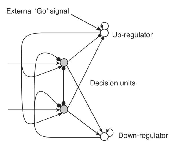
A decision making circuit of sigmoidal filter units (gray units) regulated by integral feedback control units (white units). These units integrate the error between the sum of decision making unit activity and the desired decision plane placement. The inhibitory down-regulator has a small time constant and rapid dynamics, so that it approximates a proportional feedback control device that switches on only when the sum of gray unit activity exceeds a threshold. The excitatory up-regulator has a large time constant and relatively slow dynamics, so that a small sum of gray unit activation does not produce rapid upregulation; after all, decision processes that start at the origin take time to reach symbol regions of the phase plane. Boosting net excitation of the gray units too rapidly would produce overshoot of the desired sum of activity, and instability involving oscillations of the upand down-regulators.
The units that perform this feedback control (shown in Fig. 21) are simple, self-exciting units that ramp up nearly linearly in activation at a rate determined by the error magnitude. Specifically, these controller units integrate the amount by which error exceeds a threshold determined by the units’ bias terms, β. This linear ramping can be achieved by precisely balancing recurrent self-excitation against the leak term of Eq. 3, which is also the basis of the interval timing mechanism discussed in the supplementary materials. The inputs to these units consist of an equally weighted sum of the activation of the decision-making units — this is equivalent to the average activation level in the WTA network. A pooled inhibitor is excited by positively weighted connections from the WTA units, returning inhibition in proportion to the excess of average WTA network activation above the desired level. A pooled exciter has a low bias term so that its activation in the absence of inhibition is near 1. This unit is inhibited in proportion to the average activation of the WTA network, and returns excitation in proportion to the deficit of average WTA network activation below the desired level.
This prescription for a feedback controller works because it is the sum of decision unit activation — rather than the product or ‘Hopfield energy’ (Hopfield, 1984), as in Botvinick et al. (2001) — that is used to determine the feedback signal. In any symmetrically, laterally inhibiting WTA network with two units, the sum of unit activations is constant along any decision plane (because every decision plane is equivalent to a contour of the function V1 + V2, where Vi represents the activation of the ith unit). Thus, detecting the deviation from desired decision plane placement can easily be done by summing WTA unit activations, and the weighted sum input function of our leaky integrator units is already perfectly suited to this computation.
We now have a means of supplying positive or negative feedback to a WTA network (specifically, the input layer of a module) in proportion to that network’s integrated deviation from a simple reference value for average activation. We now face the standard problems that control engineers face in supplying control inputs to their systems: too small a gain on the feedback, and error is corrected too slowly, or it leaves a residual error that cannot be eliminated (steady-state error); too high a gain, and the system is liable to undergo wild oscillations in response to perturbations. In our case, this would mean a decision plane that ricochets back and forth from the origin to the upper-right corner of the phase-plane bounding box. Furthermore, we need to allow at least enough time for the system to reach the decision plane before supplying it with strong, supplementary excitation, which would then cause overshoot and oscillations, or the multiple-winner problem we are trying to avoid in the first place.
D. Voting in full generality
We now address the fully general case of ranking preferences among productions by using linear combinations of antecedent unit activations.
Formally, we wish to be able to map any binary vector of antecedent latch unit activations onto any preference ordering among consequents. This preference ordering is defined by the weight matrix connecting the antecedent units to the consequent units. If there are N antecedent units, then there are 2N unique binary activation patterns. If there are M consequent units, then there are M! distinct preference orderings. Preferences are vectors in M-space. The weight matrix is equivalent to one form of a rated voting system for expressing the preferences of a group of voters. In this analogy, a participating voter is equivalent to an active antecedent unit, and the candidates for a one-winner election are the consequent units.
In a ratings-based voting system, voters express preferences by assigning numerical preference values to each candidate, rather than an ordinal list of relative preference rankings. Unlike rankings-based voting systems, a ratings-based system is not covered by the Arrow impossibility theorem — that is, a ratings system can achieve a unique winner (even for N > 2 and M > 3, which rankings cannot) while satisfying the constraints of the Arrow theorem. These constraints describe the intuitively reasonable properties of a fair voting system (Arrow, 1950).
Nevertheless, the particular rating method we have proposed for aggregating preferences — linear combination — is highly constrained. The ith column of the M × N weight matrix that defines the interconnections between N antecedents and M consequents corresponds to the preference ratings of the ith antecedent voter for the consequent candidates. This preference rating defines a vector in the space of consequent unit inputs. An election involves using the vector sum of all active voters’ preference vectors as the input to the stochastic decision making process implemented via the competition between consequent units.
Ranked preference orderings are determined in M-space by dividing each pair of dimensions by an (M − 1)-dimension hyperplane that intersects the two dimensions–in question — call them dimension j and k — along the 45° line (the vector with element j and k equal to 1, and 0s in all other positions). These planes divide the space into regions of points which favor dimension j over k and regions in which k is favored over j (Fig. 22 illustrates such a partition in the case of 3 consequent units). Given our decision making mechanism, whenever dimension k is favored over all others, it is the most likely to win the election, as in the two-dimensional case. However, the closer this preference vector is to a boundary between regions, and the noisier the inputs are, the less likely the leading candidate is to be selected.
This voting system cannot implement arbitrary mappings from binary antecedent vectors to consequent preference-ranking partition regions. This can be shown by a simple example in which three antecedent units vote for two candidates (Fig. 23).
Suppose that we have encoded the preferences of two antecedent units — units 1 and 2 — among two consequent units — units A and B. Suppose that these preferences correspond to the vectors labeled ‘Pref1’ and ‘Pref2’ in Fig. 23. In this case, unit 1 prefers B to A (the B value of this preference is greater than its A value), and unit 2 prefers A to B. The linear superposition of these preference vectors is a point in the B > A subspace; thus the two units together have a slight preference for B over A. This preference ranking is encoded in tabular form in the third row of Table 2 as 110 → B > A.
Figure 22.
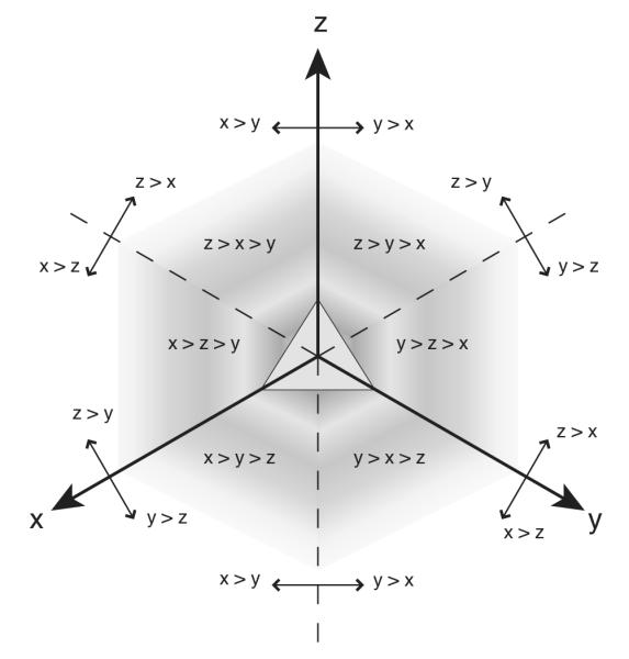
A partition of three dimensional space into 6 = 3! non-overlapping regions, each corresponding to a distinct preference ranking. The perspective is toward the origin down the vector (1,1,1), which points directly out of the page.
Now suppose we attempt to add an additional antecedent unit, unit 3, and to connect it to the consequent units in order to encode 101 → A > B, 011 → A > B and 111 B > A. → This set of context-dependent rankings cannot be implemented given the existing preferences of units 1 and 2. Fig. 13 shows graphically how existing preferences define linear constraints that separate the plane of consequent unit activations into feasible and infeasible regions (respectively, regions where a new voter’s preferences lead or fail to lead to a desired net preference ranking, given existing preferences). The intersection of the feasible half-planes defined by the set of productions in Table 2 is necessarily the empty set, regardless of the numerical ratings involved.
This example highlights what appears at first to be an unavoidable contrast between the behavior of our proposed implementation and the behavior of typical production systems. In Soar, when there is a match of multiple rules that propose different candidate operators, preference information is used to determine which operators are selected. ACT-R uses a system based on the activation levels associated with chunks and production utility values associated with rules themselves to determine which single rule to fire. The precise definition of chunks, operators and so forth is unimportant for our purposes. What is important is that in both systems, some method of rating productions numerically leads to a ranking, after which the highest-ranked production or operator is selected.
Our choice of production implementation derives, instead, directly from our model of neural processing: inputs to a unit are weighted by connection strengths and summed together to define the net input to a unit at any given moment. For this reason, it will be impossible for us to make a qualitative distinction between matching and firing. In contrast to the allor-none behavior of rules in Soar and ACT-R, every matching rule under our implementation necessarily exerts at least some miniscule influence on the outcome probabilities of a decision. Furthermore, a full match is not necessary to exert this influence: graded levels of activation in antecedent units produce a graded preference effect. The result is that the ranking operation that is carried out by the attractor dynamics within the consequent modules of all matching productions will be applied to a linear combination of the preferences supplied by the matching antecedents, rather than to a list of the preferences themselves. In another divergence from some production systems (e.g., ACT-R), only those consequents that conflict with each other are ranked in a single ranking; if two consequents A and B of matching productions do not conflict with each other and are the highest-ranked consequents among those with which they do conflict, then A and B will both be executed in parallel. Like EPIC (Meyer and Kieras, 1997) in this respect, the architecture we propose has no inherent, central cognitive bottleneck (although it can be structured, like our Tower of London model, to have a single bottleneck if desired).
Table 2.
Preference orderings of three antecedent units, 1, 2 and 3, among candidate consequent units A and B. The preferences of unit 1 are exerted on the outcome (i.e., unit 1 votes) whenever there is a 1 in the first column, labeled Pref1; this corresponds to a state of high activity in unit 1; a 0 corresponds to inactivity and no voting. The same is true for units 2 and 3. Rankings among A and B can depend on which subsets of antecedents are voting.
| Pref 1 | Pref 2 | Pref 3 | Aggregate preference ranking | |
|---|---|---|---|---|
| 1 | 0 | 0 | → | B > A |
| 0 | 1 | 0 | → | A > B |
| 1 | 1 | 0 | → | B > A |
| 1 | 0 | 1 | → | A > B |
| 0 | 1 | 1 | → | A > B |
| 1 | 1 | 1 | → | B > A |
The first of these two properties of our implementation — linear combination — is a difficulty when viewed from the perspective of a literal mapping of production systems onto neural networks. Depending on the particular production system architecture involved (i.e., whether rules are allowed to fire in parallel), the second one may be as well. These differences serve as predictions of our proposed architecture that are distinct from those of general production systems.
However, something quite like standard, Soar-style preference information can nevertheless be encoded by connection strengths in a neural network. A straightforward method can furthermore be used to assign connection strengths so that the outcome rankings are those desired by a programmer (or possibly learned by a learning algorithm, although we do not model connection-strength learning here). In this way, we can always
Figure 23.

A simple example of infeasible explicit preferences (arrow-head vectors, Pref 1, Pref 2 and Pref 3), and the emergent preferences generated by their combinations (circle-head vectors). The open circle represents an emergent preference rating of the combination of Pref 1, Pref 2 and Pref 3. This rating generates a ranking of consequent 1 higher than consequent 2. However, this ranking conflicts with any explicitly programmed production that matches antecedents 1 through 3, yet specifies a rating that ranks the alternative outcome (consequent 2) higher. In order to make such a system of explicit ratings feasible, we add a conjunction detector (a binary AND gate) to the pool of consequent units, Pref 2 ⋀ 3.
translate a set of productions into a neural network that produces identical behavior by taking sufficiently many steps to compensate for the disparities that arise from the linear combination of preferences prior to ranking. However, one virtue of the mapping that we propose is that it gives rise to emergent behaviors (behaviors not explicitly specified by the rule set) when these compensating steps are not taken.
Footnotes
For an intuitive example of leaky integration, consider a water-bucket with a hole in the bottom: when water is poured in at a fast enough rate, the height of the water approaches a stable equilibrium; after the inflow is shut off, the accumulated water drains out in such a way that its level approaches zero; and rapid changes in the input signal (the inflow of water) translate into gradual changes in the height. Reading off the water height therefore gives a smoothed version of the input signal in which high frequencies are attenuated.
Unfortunately, increased noise reduction comes at the cost of slower operation, so that higher computer speeds can be achieved by reducing capacitance and boosting power to more clearly distinguish noisy 1s from noisy 0s.
Importantly, given that our model consists of first-order differential equations, the energy surface determines the velocity of the ball, rather than its acceleration, as in the case of a real ball.
In previous work (Simen et al., 2004), we speculated that the laminar and columnar structure of mammalian cortex reflected this sort of organization, with middle and deep layers of cortex within a cortical column corresponding to the input stage, and superficial layers corresponding to the output stage, or gate.
We use the term ‘production system’ to refer to any architecture sharing the basic structural features of if-then rules and a working memory. Under our interpretation, this also includes systems referred to as ‘classifier systems’ (Holland, 1986b), and probably others.
E.g., separated by equal intervals of duration i, with Δi+1 reduced to Δi/2 at the ith reduction of the inter-sample interval.
That is, set according to Eq. 18 — with αi defined by 1 − αi ≈ exp(−Δi/τ)/2, with τ defined by Eq. 19.
We keep c constant for simplicity, but a variable c may be more plausible. In the case of thermal noise in electrical circuits, it depends on the amount of heat generated by voltage across resistors (Gardiner, 2004), and in the case of neuronal circuits, it may increase with the firing rate.
We can also solve it analytically when s is a constant. In such a case, Eq. 21 is a stochastic process — specifically, an Ornstein-Uhlenbeck process — with an asymptotic mean value given by Eq. 19, and standard deviation c/τ (Gardiner, 2004).
In the case of more than two competing processes, asymptotically optimal algorithms exist for which a neural implementation has also been proposed (Bogacz and Gurney, 2007).
References
- Ackley DH, Hinton GE, Sejnowski TJ. A learning algorithm for Boltzmann machines. Cognitive Science. 1985;9:147–169. [Google Scholar]
- Aldridge JW, Berridge KC. Coding of serial order by neostriatal neurons: a ‘natural action’ approach to movement sequence. Journal of Neuroscience. 1998;18(7):2777–2787. doi: 10.1523/JNEUROSCI.18-07-02777.1998. [DOI] [PMC free article] [PubMed] [Google Scholar]
- Alexander GE, DeLong MR, Strick PL. Parallel organization of functionally segregated circuits linking basal ganglia and cortex. Annual Review of Neuroscience. 1986;9:357–381. doi: 10.1146/annurev.ne.09.030186.002041. [DOI] [PubMed] [Google Scholar]
- Amit D, Gutfreund H, Sompolinsky H. Storing infinite numbers of patterns in a spin-glass model of neural networks. Physical Review Letters. 1985;5:1530–1533. doi: 10.1103/PhysRevLett.55.1530. [DOI] [PubMed] [Google Scholar]
- Anderson J, Lebiere C. The Atomic Components of Thought. Lawrence-Erlbaum Associates; 1998. [Google Scholar]
- Anderson JA, Silverstein JW, Ritz SA, Jones RS. Distinctive features, categorical perception, and probability learning: some applications of a neural model. Psychological Review. 1977;84:413–451. [Google Scholar]
- Anderson JR, Bothell D, Byrne MD, Douglass S, Lebiere C, Qin Y. An integrated theory of mind. Psychological Review. 2004;111(4):1036–1060. doi: 10.1037/0033-295X.111.4.1036. [DOI] [PubMed] [Google Scholar]
- Arrow KJ. A di culty in the concept of social welfare. Journal of Political Economy. 1950;58(4):328–346. [Google Scholar]
- Bader S, Hitzler P, Holldobler S, Witzel A. The Core method for first-order logic programs. Springer; Heidelberg: 2007. Ch. 9. [Google Scholar]
- Bishop C. Pattern recognition and machine learning. Springer; New York, NY: 2006. [Google Scholar]
- Bogacz R, Brown E, Moehlis J, Holmes P, Cohen JD. The physics of optimal decision making: a formal analysis of models of performance in two-alternative forced choice tasks. Psychological Review. 2006;113(4):700–765. doi: 10.1037/0033-295X.113.4.700. [DOI] [PubMed] [Google Scholar]
- Bogacz R, Gurney K. The basal ganglia and cortex implement optimal decision making between alternative actions. Neural Computation. 2007;19:442–477. doi: 10.1162/neco.2007.19.2.442. [DOI] [PubMed] [Google Scholar]
- Botvinick MM, Braver TS, Barch DM, Carter CS, Cohen JD. Conflict monitoring and cognitive control. Psychological Review. 2001;108(3):624–652. doi: 10.1037/0033-295x.108.3.624. [DOI] [PubMed] [Google Scholar]
- Braver TS, Cohen JD. On the control of control: the role of dopamine in regulating prefrontal function and working memory. In: Monsell S, Driver J, editors. Control of Cognitive Processes: Attention and Performance XVIII. MIT Press; 2000. [Google Scholar]
- Brown E, Gao J, Holmes P, Bogacz R, Gilzenrat M, Cohen JD. Simple neural networks that optimize decisions. International Journal of Bifurcation and Chaos. 2005;15(3):803–826. [Google Scholar]
- Carlin D, Bonerba J, Phipps M, Alexander G, Shapiro M, Grafman J. Planning impairments in frontal lobe dementia and frontal lobe lesion patients. Neuropsychologia. 2000;38:655–665. doi: 10.1016/s0028-3932(99)00102-5. [DOI] [PubMed] [Google Scholar]
- Cohen JD, Dunbar K, McClelland JL. On the control of automatic processes: a parallel distributed processing account of the Stroop effect. Psychological Review. 1990;97(3):332–361. doi: 10.1037/0033-295x.97.3.332. [DOI] [PubMed] [Google Scholar]
- Cohen M, Grossberg S. Absolute stability of global pattern formation and parallel memory storage by competitive neural networks. IEEE Transactions on Systems, Man and Cybernetics. 1983;13:815–826. [Google Scholar]
- Cooper R, Shallice T. Contention scheduling and the control of routine activities. Cognitive Neuropsychology. 2000;17(4):297–338. doi: 10.1080/026432900380427. [DOI] [PubMed] [Google Scholar]
- Cowan JD. Ph.D. thesis. University of London; 1967. A Mathematical Theory of Central Nervous Activity. [Google Scholar]
- Cragg BG, Temperley HNV. Memory – The analogy with ferromagnetic hysteresis. Brain. 1955;78(2):304–315. doi: 10.1093/brain/78.2.304. [DOI] [PubMed] [Google Scholar]
- Cybenko G. Approximation by superpositions of a sigmoidal function. Mathematics of Control, Signals, and Systems. 1989;2:303–314. [Google Scholar]
- Dayan P, Abbott LF. Theoretical Neuroscience: Computational and Mathematical Modeling of Neural Systems. MIT Press; Cambridge, MA: 2001. [Google Scholar]
- Dehaene S, Changeux J. A hierarchical neuronal network for planning behavior. Proceedings of the National Academy of Sciences, USA. 1997;94:13293–13298. doi: 10.1073/pnas.94.24.13293. [DOI] [PMC free article] [PubMed] [Google Scholar]
- Desimone R, Duncan J. Neural mechanisms of selective visual attention. Annual Review of Neuroscience. 1995;18:193–222. doi: 10.1146/annurev.ne.18.030195.001205. [DOI] [PubMed] [Google Scholar]
- Eliasmith C, Anderson CH. Neural Engineering: Computation, Representation, and Dynamics in Neurobiological Systems. MIT Press; Cambridge, MA: 2003. [Google Scholar]
- Feldman JA, Ballard DH. Connectionist models and their properties. Cognitive Science. 1982;6:205–254. [Google Scholar]
- Frank MJ, Loughry B, O’Reilly RC. Interactions between frontal cortex and basal ganglia in working memory: a computational model. Cognitive, A ective and Behavioral Neuroscience. 2001;1(2):137–160. doi: 10.3758/cabn.1.2.137. [DOI] [PubMed] [Google Scholar]
- Franklin GF, Powell JD, Emami-Naeini A. Feedback Control of Dynamic Systems. Addison-Wesley; New York: 1994. [Google Scholar]
- Frey PW, Sears RJ. Model of conditioning incorporating the Rescorla-Wagner associative axiom, a dynamic attention process, and a catastrophe rule. Psychological Review. 1978;85:321–340. [Google Scholar]
- Gardiner CW. Handbook of stochastic methods. 3rd Edition Springer-Verlag; New York, NY: 2004. [Google Scholar]
- Gerstner W. Population dynamics of spiking neurons: fast transients, asynchronous states, and locking. Neural Computation. 2000;12:43–89. doi: 10.1162/089976600300015899. [DOI] [PubMed] [Google Scholar]
- Goel V, Pullara SD, Grafman J. A computational model of frontal lobe dysfunction: working memory and the tower of hanoi task. Cognitive Science. 2001;25:287–313. [Google Scholar]
- Gold JI, Shadlen MN. Neural computations that underlie decisions about sensory stimuli. Trends in Cognitive Science. 2001;5(1):10–16. doi: 10.1016/s1364-6613(00)01567-9. [DOI] [PubMed] [Google Scholar]
- Gold JI, Shadlen MN. Banburismus and the brain: decoding the relationship between sensory stimuli, decisions, and reward. Neuron. 2002;36(2):299–308. doi: 10.1016/s0896-6273(02)00971-6. [DOI] [PubMed] [Google Scholar]
- Gray RM, Neuho DL. Quantization. IEEE Transactions on Information Theory. 1998;44:2325–2383. [Google Scholar]
- Green DM, Swets JA. Signal Detection Theory and Psychophysics. Wiley; New York: 1966. [Google Scholar]
- Grice GR. Application of a variable criterion model to auditory reaction time as a function of the type of catch trial. Perception and Psychophysics. 1972;102:103–107. [Google Scholar]
- Grossberg S. Biological competition: Decision rules, pattern formation and oscillations. Proceedings of the National Academy of Sciences U S A. 1980a;77(4):2338–2342. doi: 10.1073/pnas.77.4.2338. [DOI] [PMC free article] [PubMed] [Google Scholar]
- Grossberg S. How does a brain build a cognitive code? Psychological Review. 1980b;87:1–51. doi: 10.1007/978-94-009-7758-7_1. [DOI] [PubMed] [Google Scholar]
- Grossberg S. A psychophysiological theory of reinforcement, drive, motivation and attention. Journal of Theoretical Neurobiology. 1982;1:286–369. [Google Scholar]
- Grossberg S. Competitive learning: from interactive activation to adaptive resonance. Cognitive Science. 1987;11:23–63. [Google Scholar]
- Hammer B, Hitzler P, editors. Perspectives of Neural-Symbolic Integration. Springer; Heidelberg: 2007. [Google Scholar]
- Hanes DP, Schall JD. Neural control of voluntary movement initiation. Science. 1996;274(5286):427–430. doi: 10.1126/science.274.5286.427. [DOI] [PubMed] [Google Scholar]
- Harth EM, Csermely TJ, Beek B, Lindsay RD. Brain functions and neural dynamics. Journal of Theoretical Biology. 1970;26:93–120. doi: 10.1016/s0022-5193(70)80035-2. [DOI] [PubMed] [Google Scholar]
- Hartline HK, Ratli F. Inhibitory interaction of receptor units in the eye of Limulus. Journal of General Physiology. 1957;40(3):357–376. doi: 10.1085/jgp.40.3.357. [DOI] [PMC free article] [PubMed] [Google Scholar]
- Hayes J. Introduction to Digital Logic Design. Addison-Wesley; New York, NJ: 1993. [Google Scholar]
- Hertz J, Krogh A, Palmer RG. Introduction to the Theory of Neural Computation. Vol. 1 of Santa Fe Institute Studies in the Sciences of Complexity Lecture Notes. Addison Wesley; Redwood City, CA: 1991. [Google Scholar]
- Higham DJ. An algorithmic introduction to numerical simulation of stochastic differential equations. Society for Industrial and Applied Mathematics Review. 2001;43(3):525–546. [Google Scholar]
- Hodgkin AL, Huxley AF. Resting and action potentials in single nerve fibres. Journal of Physiology. 1945;104:176–195. doi: 10.1113/jphysiol.1945.sp004114. [DOI] [PMC free article] [PubMed] [Google Scholar]
- Hodgkin AL, Huxley AF. A quantitative description of membrane current and its application to conduction and excitation in nerve. Journal of Neurophysiology (London) 1952;117:500–544. doi: 10.1113/jphysiol.1952.sp004764. [DOI] [PMC free article] [PubMed] [Google Scholar]
- Holland JH. Escaping brittleness: the possibilities of general-purpose learning algorithms applied to parallel rule-based systems. In: Michalski RS, Carbonell JG, Mitchell TM, editors. Machine Learning: An Artificial Intelligence Approach. Vol. 2. Morgan Kaufmann; Los Altos, CA: 1986a. [Google Scholar]
- Holland JH. A mathematical framework for studying learning in classifier systems. Physica D. 1986b;2:307–317. [Google Scholar]
- Holmes P, Brown E, Moehlis J, Bogacz R, Gao J, Aston-Jones G. Optimal decisions: from neural spikes, through stochastic differential equations, to behavior. IEICE Transactions on Fundamentals of Electronics, Communications and Computer Science. 2005;88(10):2496–2503. [Google Scholar]
- Hopfield JJ. Neurons with graded response have collective computational properties like those of two-state neurons. Proceedings of the National Academy of Sciences, USA. 1984;81:3088–3092. doi: 10.1073/pnas.81.10.3088. [DOI] [PMC free article] [PubMed] [Google Scholar]
- Hummel JE, Holyoak KJ. Distributed representations of structure: a theory of analogical access and mapping. Psychological Review. 1997;104(3):427–466. [Google Scholar]
- Jordan DW, Smith P. Nonlinear Ordinary Differential Equations. 3rd Edition Oxford University Press; New York, NY: 1999. [Google Scholar]
- Just MA, Carpenter PA. A capacity theory of comprehension: individual differences in working memory. Psychological Review. 1992;99(1):122–149. doi: 10.1037/0033-295x.99.1.122. [DOI] [PubMed] [Google Scholar]
- Kieras D, Meyer D. An overview of the EPIC architecture for cognition and performance with application to human-computer interaction. Human Computer Interaction. 1997;12(4):391–438. [Google Scholar]
- Kimberg DY, Farah MJ. A unified account of cognitive impairments following frontal lobe damage: the role of working memory in complex, organized behavior. Journal of Experimental Psychology: General. 1993;122:411–428. doi: 10.1037//0096-3445.122.4.411. [DOI] [PubMed] [Google Scholar]
- Kleene SC. Representation of events in nerve nets and finite automata. In: Shannon CE, McCarthy J, editors. Automata Studies. Princeton University Press; Princeton, NJ: 1956. pp. 3–41. [Google Scholar]
- Laird J, Congdon CB. The Soar User’s Manual. 8th Edition Electrical Engineering and Computer Science Department; Ann Arbor, Michigan: 2006. [Google Scholar]
- Laird J, Newell A, Rosenbloom P. Soar: an architecture for general intelligence. Artificial Intelligence. 1987;33(1):1–64. [Google Scholar]
- Laird J, Rosenbloom P, Newell A. Chunking in Soar: the anatomy of a general learning mechanism. Machine Learning. 1986;1:11–46. [Google Scholar]
- Laming DRJ. Information theory of choice reaction time. Wiley; New York: 1968. [Google Scholar]
- Lapique L. Recherches quantitatives sur l’excitation électrique des nerfs traitée comme une polarization. Journal of Physiology, Pathology and Genetics. 1907;9:620–635. [Google Scholar]
- Loewenstein Y, Seung HS. Operant matching is a generic outcome of synaptic plasticity based on the covariance between reward and neural activity. Proceedings of the National Academy of Sciences U S A. 2006 October;103(41):15224–15229. doi: 10.1073/pnas.0505220103. [DOI] [PMC free article] [PubMed] [Google Scholar]
- Luce RD. Response Times: Their Role in Inferring Elementary Mental Organization. Oxford University Press; New York: 1986. [Google Scholar]
- Marcus G. The Algebraic Mind: Integrating Connectionism and Cognitive Science. MIT Press; cambridge: 2001. ma Edition. [Google Scholar]
- Marr D. Vision: A Computational Investigation into the Human Representation and Processing of Visual Information. W. H. Freeman and Company; San Francisco: 1982. [Google Scholar]
- McClelland JL, Rumelhart DE. An interactive activation model of context effects in letter perception: Part 1. An account of basic findings. Psychological Review. 1981;99:375–407. [PubMed] [Google Scholar]
- McCulloch W, Pitts W. A logical calculus of the ideas immanent in nervous activity. Bulletin of Mathematical Biophysics. 1943;5:115–133. [PubMed] [Google Scholar]
- McMillen T, Holmes P. The dynamics of choice among multiple alternatives. Journal of Mathematical Psychology. 2006;50:30–57. [Google Scholar]
- Mead C. Analog VLSI and Neural Systems. Addison-Wesley; New York: 1989. [Google Scholar]
- Meck WH. Neuropharmacology of timing and time perception. Cognitive Brain Research. 1996;3:227–42. doi: 10.1016/0926-6410(96)00009-2. [DOI] [PubMed] [Google Scholar]
- Meyer DE, Kieras DE. A computational theory of executive cognitive processes and multiple-task performance: Part 1. basic mechanisms. Psychological Review. 1997;104:3–65. doi: 10.1037/0033-295x.104.1.3. [DOI] [PubMed] [Google Scholar]
- Miller E, Cohen JD. An integrative theory of prefrontal cortex function. Annual Review of Neuroscience. 2001;24:167–202. doi: 10.1146/annurev.neuro.24.1.167. [DOI] [PubMed] [Google Scholar]
- Miller GA. The magical number seven, plus or minus two: some limits on our capacity for processing information. Psychological Review. 1956;63:81–97. [PubMed] [Google Scholar]
- Miller GA, Galanter E, Pribram KH. Plans and the Structure of Behavior. Holt, Rinehart & Winston; 1960. [Google Scholar]
- Montague PR, Berns GS. Neural economics and the biological substrates of valuation. Neuron. 2002 October;36:265–284. doi: 10.1016/s0896-6273(02)00974-1. [DOI] [PubMed] [Google Scholar]
- Nakahara H, Doya K. Near-saddle-node bifurcation behavior as dynamics in working memory for goal-directed behavior. Neural Computation. 1998;10:113–132. doi: 10.1162/089976698300017917. [DOI] [PubMed] [Google Scholar]
- Newell A. Unified Theories of Cognition. Harvard University Press; Cambridge, MA: 1990. [Google Scholar]
- Newell A, Simon H. Human Problem-Solving. Prentice Hall; Englewood Cliffs, NJ: 1972. [Google Scholar]
- Newell A, Simon HA. GPS: A program that simulates human thought. In: Feigenbaum EA, editor. Computers and Thought. McGraw-Hill; New York: 1963. [Google Scholar]
- Oksendal B. Stochastic Di erential Equations. Springer; 2003. [Google Scholar]
- Oppenheim AV, Willsky AS. Signals and systems. 2nd Edition Prentice Hall; New York, NY: 1996. [Google Scholar]
- O’Reilly RC, Busby RS, Dietterich T. Generalizable relational binding from coarse-coded distributed representations. In: Becker S, Ghahramani Z, editors. Advances in Neural Information Processing. Vol. 14. MIT Press; Cambridge, MA: 2002. [Google Scholar]
- O’Reilly RC, Munakata Y. Computational Explorations in Cognitive Neuroscience: Understanding the Mind by Simulating the Brain. MIT Press; 2000. [Google Scholar]
- Owen AM, Downes JJ, Sahakian BJ, Polkey CE, Robbins TW. Planning and spatial working memory following frontal lobe lesions in man. Neuropsychologia. 1990;28(10):1021–1034. doi: 10.1016/0028-3932(90)90137-d. [DOI] [PubMed] [Google Scholar]
- Owen AM, James M, Leigh PN, Summers BA, Marsden CD, Quinn NP, Lange KW, Robbins TW. Fronto-striatal cognitive deficits at different stages of parkinson’s disease. Brain. 1992;115:1727–1751. doi: 10.1093/brain/115.6.1727. [DOI] [PubMed] [Google Scholar]
- Owen AM, Sahakian BJ, Hodges JR, Summers BA, Polkey CE, Robbins TW. Dopamine-dependent frontostriatal planning deficits in early parkinson’s disease. Neuropsychology. 1995;9(1):126–140. [Google Scholar]
- Polk TA, Drake RM, Jonides JJ, Smith MR, Smith EE. Attention enhances the neural processing of relevant features and suppresses the processing of irrelevant features in humans: a functional magnetic resonance imaging study of the Stroop task. Journal of Neuroscience. 2008;28:13786–13792. doi: 10.1523/JNEUROSCI.1026-08.2008. [DOI] [PMC free article] [PubMed] [Google Scholar]
- Polk TA, Simen PA, Lewis RL, Freedman EG. A computational approach to control in complex cognition. Cognitive Brain Research. 2002;15(1):71–83. doi: 10.1016/s0926-6410(02)00217-3. [DOI] [PubMed] [Google Scholar]
- Poor HV. An Introduction to Signal Detection and Estimation. Springer-Verlag; New York: 1994. [Google Scholar]
- Ratcliff R. A theory of memory retrieval. Psychological Review. 1978;85:59–108. [Google Scholar]
- Ratcliff R, Rouder JN. Modeling response times for two-choice decisions. Psychological Science. 1998;9:347–356. [Google Scholar]
- Reddi BAJ, Carpenter RHS. The influence of urgency on decision time. Nature. 2000;3(8):827–830. doi: 10.1038/77739. [DOI] [PubMed] [Google Scholar]
- Ritter H, Haschke R, Steil JJ. A dual interaction perspective for robot cognition: grasping as a “Rosetta Stone”. In: Hammer B, Hitzler P, editors. Perspectives of Neural-Symbolic Integration. Springer; Berlin: 2007. pp. 159–178. [Google Scholar]
- Roe RM, Busemeyer JR, Townsend JT. Multialternative decision field theory: a dynamic connectionist model of decision making. Psychological Review. 2001;108(2):370–392. doi: 10.1037/0033-295x.108.2.370. [DOI] [PubMed] [Google Scholar]
- Roitman JD, Shadlen MN. Response of neurons in the lateral intraparietal area during a combined visual discrimination reaction time task. Journal of Neuroscience. 2002;22(21):9475–9489. doi: 10.1523/JNEUROSCI.22-21-09475.2002. [DOI] [PMC free article] [PubMed] [Google Scholar]
- Rosenblatt F. The perceptron: a probabilistic model for information storage and organization in the brain. Psychological Review. 1958;65:386–408. doi: 10.1037/h0042519. reprinted in Anderson and Rosenfeld(1988) [DOI] [PubMed] [Google Scholar]
- Rumelhart DE, Hinton GE, Williams RJ. Learning representations by back-propagating errors. Nature. 1986;323:533–536. [Google Scholar]
- Seung HS, Lee DD, Reis BY, Tank DW. The autapse: a simple illustration of short-term analog memory storage by tuned synaptic feedback. Journal of Computational Neuroscience. 2000;9:171–185. doi: 10.1023/a:1008971908649. [DOI] [PubMed] [Google Scholar]
- Shadlen MN, Newsome WT. The variable discharge of cortical neurons: implications for connectivity, computation, and information coding. Journal of Neuroscience. 1998;18(10):3870–3896. doi: 10.1523/JNEUROSCI.18-10-03870.1998. [DOI] [PMC free article] [PubMed] [Google Scholar]
- Shadlen MN, Newsome WT. Neural basis of a perceptual decision in the parietal cortex (area LIP) of the rhesus monkey. Journal of Neurophysiology. 2001;86(4):1916–1936. doi: 10.1152/jn.2001.86.4.1916. [DOI] [PubMed] [Google Scholar]
- Shallice T. Specific impairments in planning. Philosophical Transactions of the Royal Society of London, Series B. 1982;298:199–209. doi: 10.1098/rstb.1982.0082. [DOI] [PubMed] [Google Scholar]
- Shastri L, Ajjanagadde V. From simple associations to systematic reasoning: a connectionist representation of rules, variables and dynamic bindings using temporal synchrony. Behavioral and Brain Sciences. 1993;16:417–494. [Google Scholar]
- Simen PA, Cohen JD. Explicit melioration by a neural diffusion model. Brain Research. doi: 10.1016/j.brainres.2009.07.017. in press. [DOI] [PMC free article] [PubMed] [Google Scholar]
- Simen PA, Cohen JD, Holmes P. Rapid decision threshold modulation by reward rate in a neural network. Neural Networks. 2006;19:1013–1026. doi: 10.1016/j.neunet.2006.05.038. [DOI] [PMC free article] [PubMed] [Google Scholar]
- Simen PA, Polk TA, Lewis RL, Freedman E. A computational account of latency impairments in problem solving by Parkinson’s patients; Proceedings of the International Conference on Cognitive Modeling.2004. pp. 273–279. [Google Scholar]
- Simen PA, Polk TA, Lewis RL, Freedman EG. Universal computation by networks of model cortical columns; Proceedings of the International Joint Conference on Neural Networks.2003. pp. 230–235. [Google Scholar]
- Simon HA. The functional equivalence of problem solving skills. Cognitive Psychology. 1975;7:268–288. [Google Scholar]
- Sipser M. Introduction to the Theory of Computation. PWS Publishing Co.; Boston, MA: 1997. [Google Scholar]
- Smith PL, Ratcliff R. Psychology and neurobiology of simple decisions. Trends in Neuroscience. 2004;27:161–168. doi: 10.1016/j.tins.2004.01.006. [DOI] [PubMed] [Google Scholar]
- Soltani A, Wang XJ. A biophysically based neural model of matching law behavior: melioration by stochastic synapses. Journal of Neuroscience. 2006;26(14):3731–3744. doi: 10.1523/JNEUROSCI.5159-05.2006. [DOI] [PMC free article] [PubMed] [Google Scholar]
- Sparso J, Furber S. Principles of Asynchronous Circuit Design. Springer; 2002. [Google Scholar]
- Stone M. Models for choice reaction time. Psychometrika. 1960;25:251–260. [Google Scholar]
- Sun R, Coward LA, Zenzen MJ. On levels of cognitive modeling. Philosophical Psychology. 2005;18(5):613–637. [Google Scholar]
- Sutherland I, Ebergen J. Computers without clocks. Scientific American. 2002 May;:62–69. doi: 10.1038/scientificamerican0802-62. [DOI] [PubMed] [Google Scholar]
- Sutton RS, Barto AG. Reinforcement Learning. MIT Press; Cambridge, MA: 1998. [Google Scholar]
- Thom R. Structural Stability and Morphogenesis: An Outline of a General Theory of Models. Addison-Wesley; Reading, MA: 1989. [Google Scholar]
- Touretzky DS. BoltzCONS: dynamic symbol structures in a connectionist network. Artificial Intelligence. 1990;46:5–46. [Google Scholar]
- Touretzky DS, Hinton GE. A distributed connectionist production system. Cognitive Science. 1988;12(3):423–466. [Google Scholar]
- Usher M, McClelland JL. The time course of perceptual choice: the leaky, competing accumulator model. Psychological Review. 2001;108(3):550–592. doi: 10.1037/0033-295x.108.3.550. [DOI] [PubMed] [Google Scholar]
- Von Neumann JV, Morgenstern O. Theory of Games and Economic Behavior. Princeton University Press; Princeton, N.J.: 1944. [Google Scholar]
- Wald A, Wolfowitz J. Optimum character of the sequential probability ratio test. Annals of Mathematical Statistics. 1948;19:326–339. [Google Scholar]
- Wang XJ. Synaptic reverberation underlying mnemonic persistent activity. Trends in Neuroscience. 2001;24(8):455–463. doi: 10.1016/s0166-2236(00)01868-3. [DOI] [PubMed] [Google Scholar]
- Wang XJ. Probabilistic decision making by slow reverberation in cortical circuits. Neuron. 2002;36(5):955–968. doi: 10.1016/s0896-6273(02)01092-9. [DOI] [PubMed] [Google Scholar]
- Ward G, Allport A. Planning and problem-solving using the five-disc tower of london task. Quarterly Journal of Experimental Psycholy Section A: Human Experimental Psychology. 1997;50:49–78. [Google Scholar]
- Williams RJ, Zipser D. A learning algorithm for continually running fully recurrent neural networks. Neural Computation. 1989;1:270–280. [Google Scholar]
- Wilson HR, Cowan JD. Excitatory and inhibitory interactions in localized populations of model neurons. Biophysical Journal. 1972;12:1–24. doi: 10.1016/S0006-3495(72)86068-5. [DOI] [PMC free article] [PubMed] [Google Scholar]
- Wong KF, Wang XJ. A recurrent network mechanism of time integration in perceptual decisions. Journal of Neuroscience. 2006;26(4):1314–1328. doi: 10.1523/JNEUROSCI.3733-05.2006. [DOI] [PMC free article] [PubMed] [Google Scholar]
Associated Data
This section collects any data citations, data availability statements, or supplementary materials included in this article.