Physically grounded approach for estimating gene expression from microarray data

Abstract

High-throughput technologies, including gene-expression microarrays, hold great promise for the systems-level study of biological processes. Yet, challenges remain in comparing microarray data from different sources and extracting information about low-abundance transcripts. We demonstrate that these difficulties arise from limitations in the modeling of the data. We propose a physically motivated approach for estimating gene-expression levels from microarray data, an approach neglected in the microarray literature. We separately model the noises specific to sample amplification, hybridization, and fluorescence detection, combining these into a parsimonious description of the variability sources in a microarray experiment. We find that our model produces estimates of gene expression that are reproducible and unbiased. While the details of our model are specific to gene-expression microarrays, we argue that the physically grounded modeling approach we pursue is broadly applicable to other molecular biology technologies.

One thousand manuscripts are published each year involving microarray technology.† In spite of the 15-year history of the field, those manuscripts still describe a wide variety of data analysis methods, many of them poorly specified. Indeed, criticisms of the validity and reproducibility of microarray experiments have dogged the technology since its inception. There are two possible explanations for these shortcomings: (i) inherent limitations of the microarray technology that constrain its utility or (ii) modeling strategies that are not appropriate. The former is potentially a fundamental problem that can be overcome only with technological advances. This hypothesis has led to candid speculation that emerging sequencing technologies will quickly replace microarrays as the de facto genome-wide expression analysis technique (1, 2).

An alternative view is that current shortcomings result from gaps in our understanding of how to model the data generated in microarray experiments. In order to pursue this point, let us consider the motivation for the “standard” model (3). The fluorescence intensity F_i (Fig. 1A) detected at a spot i is surmised to be the sum of a background term and a term related to the expression level E_i we want to estimate,

[1]

Oddly, the standard model assumes that B_i can be directly determined from the fluorescence intensity measured in the nonfeature region surrounding the spot.^‡ The dependence on E_i is assumed to be distorted by multiplicative noise (3). These assumptions yield

[2]

where ν^sp is normally distributed with zero mean, and A_i is a parameter capturing the effects of hybridization efficiency and dye-specific and experiment-specific factors.

Fig. 1.

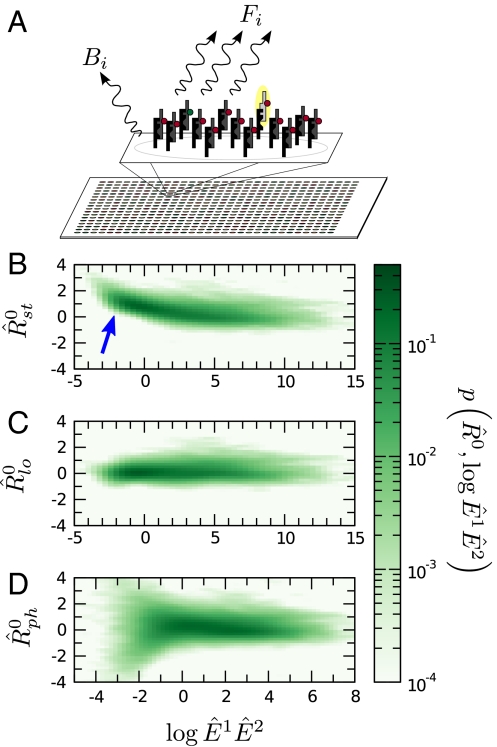
(A) Schematic of a microarray chip. Two quantities are typically reported for each spot in a two-color microarray experiment: the median feature fluorescence F_i and the median nonfeature fluorescence B_i. The total feature intensity is constituted by the sum of intended specific associations between probe and target (dark gray), as well as any number of nonspecific interactions (light gray). Because the nonfeature region has no probes attached, it is unreasonable to assume that B_i can provide reliable information on the nonspecific hybridization occurring in the feature region. (B–D) Single chip-wide joint probability distributions of and for an A. thaliana chip (19) (GEO accession no. GSM133484). (B) A plot of against is equivalent to the “MA” plots commonly used to diagnose bias in microarray data. estimates from the statistical model (Eq. 2) depend strongly on , particularly for small (blue arrow). This bias is absent from data adjusted using (C) the scatterplot smoothing routine lowess and (D) from estimates derived from our physically grounded model.

Because of the difficulty in estimating systematic effects affecting the value of A, microarray experiments are frequently performed with an internal control, the goal being to determine change of expression R_i between two conditions, 1 and 2, instead of the expression level for each condition:

[3]

where , and are the best estimates of R_i and E_i. Because, according to Eq. 2, F_i and B_i can be directly measured, the crux of the traditional approach is to estimate .

In dye-swap experiments, for which the two conditions are identical, one can develop a number of reasonable expectations for p(R_i) and p(R_i|E_i). Assuming no correlations in the values of , one expects the average value of R_i to be zero. Moreover, assuming that A_i is nonnegligible, one expects the standard deviation of R_i to decrease with increasing E_i. Unfortunately, neither of these expectations is typically obeyed by the data (Fig. 1 B, C, D).

As a result, the field has failed to converge on a single, robust model. Instead, publications reporting microarray data include a bevy of variations of this standard model. In many cases, these models were “rescued” to achieve the aforementioned expected properties by the use of idiosyncratic nonlinear corrections. Exemplifying this are the data reanalyzed in this manuscript—the authors of the studies considered have used different normalization techniques (4, 5).

Here, we argue that background fluorescence intensity cannot be correctly estimated by . Nonspecific hybridization is the dominant factor determining B_i. In order to correctly estimate B_i, we propose a dramatically distinct approach to determining gene-expression levels from microarray data. Instead of attempting to surmise a functional expression for F_i, we model each of the processes that constitute a microarray experiment. Remarkably, by propagating the fluctuations one expects in each stage of the protocol, we arrive at a concise expression relating E_i to measured quantities in the experiment.

We find that our model is able to capture the properties of microarray data for thousands of experiments. Moreover, our model yields reproducible estimates of changes in expression level.

The Physically Grounded Approach

The protocol for two-color cDNA microarray experiments is now essentially standard (6). The measurement component has three main stages, each with its own characteristics. Sample preparation consists of mRNA extraction, purification, amplification, and labeling. Hybridization is the process by which differently labeled targets bind surface-associated probes. Detection is the excitation and scanning of surface-associated fluorophores. In the following, we describe and model each of these stages.

Consider a biological sample consisting of E_i copies of transcript i, with i = 1,…,N_tr. The quantity of RNA derived from a biological sample is typically insufficient for efficient quantification by current experimental methods. Thus, sample amplification is necessary. One of two methods is typically employed to amplify the original messenger RNA: (i) expression in a T7 viral vector or (ii) polymerase chain reaction. Amplification by T7 vector expression is currently the preferred method because it results in smaller variability for high expression levels (7); thus, we consider it here (SI Text).

cDNA vectors are prepared from sample mRNAs by incorporating the T7 polymerase promoter into reverse transcriptase primers. Approximately one vector arises from each mRNA. We assume that transcription of these vectors to RNA is kinetically limited by the rate R_b of binding of T7 polymerase to transcription start sites (8). In our model, we disregard sequence or length dependent effects on transcription rate (7, 9).

In a well-mixed solution, transcripts of gene i are produced at a characteristic rate, E_iR_b. Under experimental conditions, the number of transcripts present after running the process for a time t is described by a Poisson process with parameter E_iR_bt. We expect the amplification gain to be very high, that is, R_bt≫1. In this limit, the Poisson distribution of number of transcripts arising from this process converges to a Gaussian distribution. This implies that the number n_i of copies of cDNA for gene i available for hybridization is a Gaussian variate with mean and variance equal to E_iR_bt.

Consider now competitive hybridization in a solution that is well-mixed and let p_ii be the probability of specific hybridization of target i to feature i. p_ii may depend on the sequence of gene i and on experimental conditions such as temperature and buffer concentration, but typically probe sequences are selected so that p_ii is approximately constant. Thus, we assume that p_ii = p_sp for all i and let its fluctuations be incorporated into the noise. We suggest that the number of specifically hybridized probes in the feature follows a binomial distribution with parameter p_sp. If n_ip_sp≫1, then the central limit theorem holds, and is a Gaussian variate with mean n_ip_sp,

[4]

where and are Gaussian variates with zero mean.

Similarly, let p_ji be the nonspecific hybridization efficiency for gene j to probe i. The number of hybridized probes j in feature i will then be

[5]

where is again a Gaussian variate with mean zero. Note that p_ji ≪ p_ii for all j ≠ i. The total contribution of nonspecific hybridization from all targets to the observed signal will then be

[6]

Estimating p_ji directly for all pairs of transcripts is not feasible in practice. In order to proceed, we thus use a mean-field approximation. Specifically, we assume that no single gene is responsible for a significant fraction of all mRNA targets. We further assume that p_ji is not dependent strongly on j or i; that is p_ji ≈ p^nsp. Under these assumptions, Lyapunov’s central limit theorem applies, yielding

[7]

where U^′ is the characteristic contribution of nonspecific hybridization and is a Gaussian variate with zero mean.

The fluorescence generated by the excitation of the spots on the chip will be amplified in the scanning process. Amplification using a photomultiplier is characterized by a dye-specific gain G that is a function, in principle, of dye incorporation rate, dye properties, laser power, and detector characteristics, yielding a detected fluorescence

[8]

where , the noise associated with stage k of amplification, is normally distributed with mean zero. We assume that the gain is constant and does not depend on the intensity of the signal, or on any other spot property; that is, G_i = G. We also assume that there is no specific interaction between a dye molecule and either target or probe sequence, an assumption that we find fails for some probes (SI Text).

Because the variability for each term in Eq. 8 is the product of several independent Gaussian variables, the terms will converge to a log-normal distribution. We can therefore write Eq. 8 as

[9]

where A ≡ R_btp_spG, U ≡ U^′G, and the noise terms and are normally distributed with mean zero and standard deviations σ_sp and σ_nsp.^§ Our physically grounded model thus has four parameters that relate E_i to F_i: A, U, σ_sp, and σ_nsp.

Although formally similar, Eq. 9 differs significantly from the standard statistical model typically assumed for observed feature intensity, Eq. 2. Here, B_i, the nonfeature intensity local to spot i, is measured from the data. This is in contrast to our interpretation of additive noise in a microarray experiment, which is dominated by nonspecific hybridization. Because background fluorescence and nonspecific hybridization cannot be decoupled, we explicitly model the latter.

Model Validation

We next compare the predictions of Eqs. 2 and 9 for the distribution of observed feature intensities p(F). To this end, we must surmise a functional form for the distribution of expression levels p_E(E). We expect p_E(E) to be strictly decreasing; most genes have very low expression levels, whereas a few genes have high expression levels. Following recent reports (10–12), we assume that p(E) exhibits a power law decay, such that

[10]

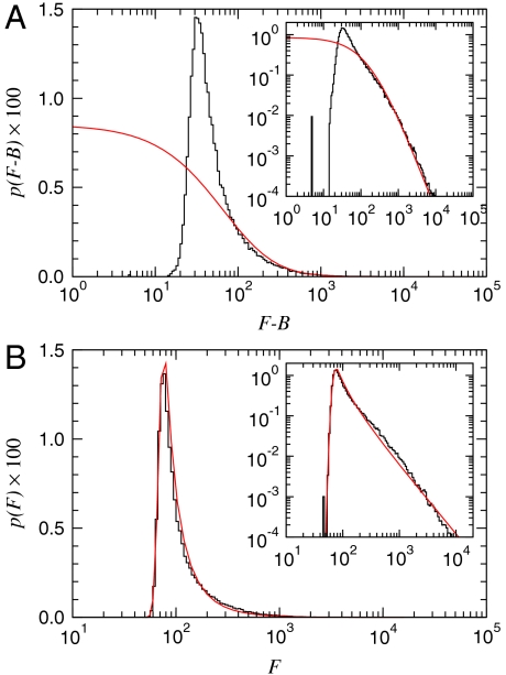
We derive p(F) for both models and obtain maximum likelihood estimates of the model parameters—including α—by the method of steepest descent (SI Text). We find that our model predicts the empirical distributions extraordinarily well, whereas the statistical model does not (Figs. 2 A and B). Note that because Eq. 2 includes two observed quantities (F_i and B_i), the distribution in Fig. 2B is expressed as a function of (F_i - B_i). For the Arabidopsis thaliana chips we considered, our results suggest that p_E(E) follows a power law decay with α ≈ 1.7, consistent with previous reports (12).

Fig. 2.

Model validation. (A) Standard statistical model, Eq. 2. The maximum likelihood parameter estimate (red) fails to reproduce the distribution of observed feature intensities (black). (B) Physically grounded model, Eq. 9. The best fit (red) agrees extraordinarily well with the empirical data (A and B Insets). The physically grounded model strongly suggests that gene-expression levels decay according to a power law with an exponent of α ≈ 1.7.

To summarize the abilities of the standard statistical model and the physically grounded model to reproduce the distributions of observed fluorescences, we fit parameters for both models to 894 Agilent gene-expression chips from the compendium of arrays in the National Center for Biotechnology Information Gene Expression Omnibus (GEO) for which raw data has been deposited. For each of these chips, we computed the error, e_m of the fit to the model,

[11]

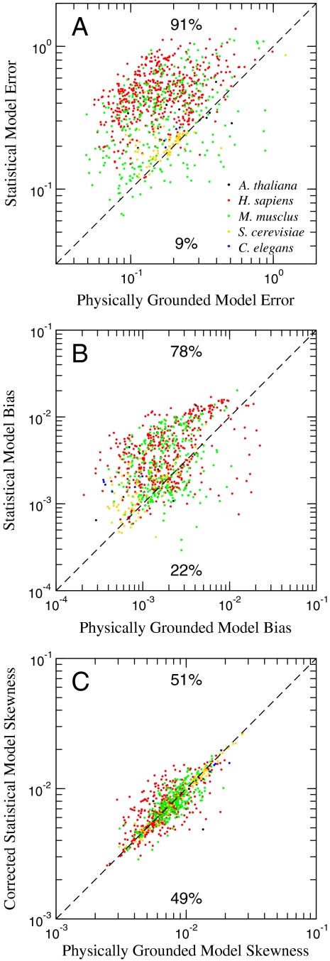
where p_e and p_m are the empirical and model-derived probability density functions, respectively. For 91% of the chips, our model results in a better description of the distribution of fluorescence intensities (Fig. 3A).

Fig. 3.

(A) Evaluation of the quality of fit between the two models and hundreds of archival microarrays reveals that the physically grounded model better represents the distribution of F_i than does the standard statistical model in 91% of the chips. The mean ratio of statistical model error to physically grounded model error is 2.73. (B) We quantified the extent of intensity-dependent dye bias in a set of 894 archived experiments. In the vast majority of these cases (78%), our physically grounded model decreased the extent of the bias, compared to the standard statistical model. Note that we are not correcting for bias due to detector saturation at high values of E. The mean ratio of bias between the statistical model and our model is 2.42. (C) Higher moments of —including skewness—are near zero and equivalent between the lowess-corrected statistical model and our physically grounded model, demonstrating that physically grounded modeling eliminates the need for nonlinear intensity-dependent bias corrections.

Intensity-Dependent Dye Bias.

Next, we consider a metric of relative expression change; see Eq. 3. In the special case that for all i—as would occur in a dye-swap experiment—one expects the distribution of R_i to be symmetric about its mean, zero. In this special case, because there is no expression change, we denote the observed R_i = R⁰ to indicate the absence of an underlying signal. We utilize data from experiments employing a dye-swap design to investigate the presence of bias in the estimation of E_i. These experiments employ a technical replicate of each sample, alternating the labeling scheme on the second replicate. This procedure yields a pair of realizations and that arise from a single set of expression levels.

A common assumption in the literature is that the gain of a dye-detector system can depend on the signal intensity in a profound way, giving rise to intensity-dependent dye bias (Fig. 1B). Because no theoretical expression exists to describe the dependence of this bias on F_i, investigators use nonlinear regression techniques such as the scatterplot smoothing algorithm lowess to correct affected data (Fig. 1C and SI Text) (13, 14).

We propose that the prevalence of this bias is due in large part to an incorrect adjustment for the additive noise in the experiment, which, after data are logarithmically transformed, manifests itself nonlinearly. We investigated the existence of intensity-dependent dye bias in estimates from our model and found that R⁰ estimates using our model show only a very weak dependence on E (Fig. 1D).

To more completely address the extent of dye bias in estimates generated from these models, we quantified its presence in the 894 microarrays described above. While these chips are not typically performed in dye-swap arrangement, the extreme heterogeneity of the sample origins motivates the assumption that R⁰ is typically zero centered and does not depend on E.

We define the extent of bias of a model, b_m,

[12]

where is the 100-point moving average of for model m. We found that this bias is greater for the estimates using the standard statistical model in 78.5% of the chips we considered (Fig. 3B).

Not surprisingly, the lowess-corrected statistical model decreases the dependence of on E, compared to the standard statistical model. However, our model yields estimates of that are no more biased than those observed with the lowess-corrected model (Fig. 3C).

Reproducibility.

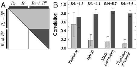
We next assess intra- and interlab experimental reproducibility. We consider microarray experiments performed at three labs with identical reference samples from two different sources (Universal Human Reference; Human Brain Reference) (4). Each lab performed five replicates of four protocols, including either competitive hybridization of the same sample or of different samples. We measured the correlation between the estimated expression level changes across protocols, replicates, and labs for our model, the standard statistical model, and the statistical model used in ref. 4. For identical samples, we expect correlations across microarray experiments to be close to zero. We find an average correlation of 0.10 using our model’s estimates. For distinct samples we expect a correlation close to 1 and find a mean correlation of 0.79 for our model’s estimates (Fig. 4).

Fig. 4.

Inter- and intralab experimental reproducibility. (A) Expression change estimates derived from our physically grounded model are consistent across intralab, interlab, and dye-swap replicates. To test this, we used published quality-control data following the design scheme described in ref. 4. Each of these four experiments was replicated five times, in three different labs (see SI Text). The experimental design included a number of technical replicates in which the same sample is labeled with different agents, such that R_i = R⁰. Because they are measurements of the absence of expression change, these dye-swap experiments are useful for assessing the specificity of the data and the model used to extract them. We estimated expression changes for four models and computed the correlation over all pairs of dye-swap chips (light gray, Fig. S3). (B) The mean correlation between R_i predicted from our physically grounded model is 0.10, lower than those derived from the statistical (Eq. 2) model, the lowess-corrected statistical model, and the MicroArray Quality Control (MAQC)-reported expression changes. The mean correlation of R_i estimates derived from chips comparing distinct commercially derived samples (R_i ≠ R⁰) was comparable for all models, but the signal-to-noise ratio (S/N) for the physically grounded model is substantially higher than for the other models. The combination of these two observations leads us to conclude that the statistical power of our model substantially surpasses existing methodologies.

Model Implications

Eq. 2 and similar models supply no direct means of determining the significance of gene-expression changes and therefore often rely on arbitrary thresholds. The intrinsic difficulty of quantitatively establishing significance of microarray results is highlighted in Fig. 1D—the scale of fluctuations varies nonlinearly with expression level. Our model enables us to quantify in a natural way the probability of rejecting the null hypothesis that a gene’s expression level is unchanged between samples. To identify genes that are expressed differentially between two samples, we consider a null model for R_i, which assumes that the expression in the two samples is identical. Specifically, given two fluorescence levels and , the probability density that the corresponding expression levels and are identical is

[13]

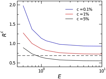
We denote the expression ratios estimated from the physically grounded and statistical models as and , respectively. One can determine the expected distribution of R⁰ values for any expression level if a gene’s expression level has not changed (SI Text). This distribution will depend on the parameter estimates for the model, but Fig. 5 shows that the confidence intervals for lower expression levels are larger than the corresponding intervals for more highly expressed genes. This is expected, because nonspecific hybridization constitutes a larger fraction of S_i (and consequently of F_i) for low E_i, resulting in R_i estimates with larger uncertainty.

Fig. 5.

Null model for expression change. By deriving the distribution p(R⁰|E), we can establish a confidence interval such that p(R^c∈R⁰|E¹ = E² = E) = 1 - c (Fig. S5). The likelihood of a particular R falling outside this confidence interval is small if the expression is not changed. This allows us to quantitatively identify genes with statistically significant expression changes. Genes with low expression have larger confidence intervals because nonspecific binding noise is more important to the estimates for these genes than for highly expressed genes. The dashed line denotes the “twofold change” traditionally used to determine significance in microarray experiments. The appropriate value of c should be dictated by an appropriate false discovery rate controlling procedure (20–22).

Enrichment of Experimental Power

To further illustrate the limitations of the current approaches and the significance of our approach, we next applied our methods to a dataset reported in ref. 5. In this study, three cohorts of animals were fed different diets: standard lab diet (SD), high-calorie, high-fat diet (HC), and the high-fat diet supplemented with the small molecule resveratrol (HCR).

Resveratrol has been shown to extend life span in several model organisms (15, 16). Baur et al. (5) suggested the existence of a molecular basis for the phenotypic similarity they observe between SD and HCR mice. As such, they performed microarray experiments to test the hypothesis that HCR animals are transcriptionally similar to SD animals.

RNA from the livers of animals from each feeding protocol were hybridized against a pool of RNA from the SD mice. From these chips we estimated (again, filtering for poor-quality spots and prevalent sequence-dependent dye bias, SI Text) using the statistical model, our physically grounded model, a lowess-corrected statistical model, and the z-score normalization used by Baur et al. (5, 17) (see SI Text). We computed the correlation between for each pair of chips for each model to understand the degree of specificity and sensitivity that each imparts and to test the hypothesis that HCR animals are transcriptionally similar to SD animals, whereas HC animals are distinct from both.

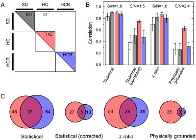
If there is a robust difference between expression changes between two samples, one expects the expression change to be consistent—a high correlation—across replicates. If there is no difference, one expects weak correlation (Fig. 6A). The similarity between the estimates derived from the statistical model for the HCR animals are statistically indistinguishable from the similarity between the control animals (Fig. 6B). The authors of ref. 5 had to use a higher-level pathway analysis (18) to distinguish between the HCR and HC mice. In contrast, estimates derived from our model strongly support the hypothesis that HCR animals are transcriptionally similar to SD animals (Fig. 6B). Our analysis indicates that the difference is clear at the level of correlation of individual gene-expression changes, an effect that is unobservable using other models. This leads us to conclude that our model imparts greater statistical power.

Fig. 6.

Enrichment of gene lists. (A) To understand the practical implications of our model, we computed correlation between pairs of estimates of different feeding protocols. These pairs of chips can be divided into four qualitatively different sets. (B) Correlations between expression change estimates calculated using the standard model (white) are high between replicates, even in SD experiments (5), resulting in weak statistical power (Fig. S7). This makes it difficult to establish that the difference between HCR and SD feeding regimens is small relative to the difference between the HC and SD regimens. In contrast, correlations between expression changes calculated using our physically grounded model (gray) have weak correlations between SD replicates, strong correlations between HC replicates, and weak correlations between HCR replicates. This conclusively indicates that the differences between HCR and SD transcriptomes are on the same order of technical noise, while there is a robust difference between HC and SD transcriptomes. (C) Consistent sets of genes up- and down-regulated genes (which we have combined for simplicity) for HC (red) and HCR (blue) chips. As expected, HCR sets derived from our physically grounded model have very little overlap because few genes have changed expression. Likewise, very few genes are common to both the HC and HCR sets, indicating that they are distinct expression patterns. S/Ns are calculated as the ratio of the mean correlation of the HC chips to the SD chips.

Having established the statistical legitimacy of our model, we investigated what practical implications it has for identifying consistent sets of up- and down-regulated transcripts. For our model and the three others, we determined the 100 genes most likely to be up- and down-regulated for each chip. For the HC and HCR chips, we aggregated genes that were represented in at least three of four sets (Fig. 6C). Given the hypothesis that HCR animals are similar to control animals, we expect that there is much less consistency between the HCR sets (i.e., small circles). Also, if the HCR and HC animals are distinct, they should have very few genes common across conditions (i.e., small overlap of the circles). This is the behavior we observe in the sets derived from our model—there is very little consistency between the HCR sets, but the HC sets are robust—but not for the other models.

Discussion

We demonstrate here that a physically grounded approach successfully models the outcome of gene-expression microarray experiments. Whereas linear models assuming normally distributed error terms may be appropriate models for many experiments in biology, they fail in many high-throughput applications due to the multiplicative nature of propagating fluctuations. For these experiments, consideration of the physical processes responsible for the outcome is essential. Our model, although constructed with two-color expression microarrays in mind, is generalizable to other systems. As chip-based assays and other high-throughput technologies continue to evolve, it will become increasingly important to establish physically grounded models for the resulting data. Although the specifics of a particular protocol may vary, a physically grounded model can be derived to understand any procedure that is composed of serial, fundamentally understood stages. For these experiments, statistical models are often the first approach because physically grounded models may be perceived as difficult to develop. In many cases, the benefits of the physically grounded modeling approach are appreciable and may outweigh increased developmental difficulty.

We have found that this approach produces a model for microarray data that reproduces macroscopic properties of the chip and results in estimates of expression changes that are nearly free of intensity-dependent dye bias, an artifact that has been traditionally rectified using ad hoc approaches. As a result, the estimates we obtain of the expression levels are systematically reproducible within and across laboratories. In addition, our model allows us to assign confidence to expression changes, even in experiments devoid of technical and biological replicates.

Our study provides yet another cautionary tale of the ad hoc adjustment of models of complex data. The standard statistical model of microarray data has many laudable features: It is simple, it has easily understood parameters, and it is readily testable. Indeed, the model’s inability to capture even basic properties of the data (Figs. 1, 2, and 3) would strongly suggest the need to reject it. Surprisingly, instead of rejecting the model, the course followed by the field has been its “rescuing” with uncontrolled and unjustified corrections. Our study shows that these corrections are unnecessary.

References

- 1.Shendure J. The beginning of the end for microarrays? Nat Methods. 2008;5:585–587. doi: 10.1038/nmeth0708-585. [DOI] [PubMed] [Google Scholar]
- 2.Ledford H. The death of microarrays? Nature. 2008;455:847. doi: 10.1038/455847a. [DOI] [PubMed] [Google Scholar]
- 3.Smyth G, Yang Y, Speed T. Statistical issues in cDNA microarray data analysis. Method Mol Biol. 2003;224:111–136. doi: 10.1385/1-59259-364-X:111. [DOI] [PubMed] [Google Scholar]
- 4.Shi LM, et al. The MicroArray Quality Control (MAQC) project shows inter- and intraplatform reproducibility of gene expression measurements. Nat Biotechnol. 2006;24:1151–1161. doi: 10.1038/nbt1239. [DOI] [PMC free article] [PubMed] [Google Scholar]
- 5.Baur JA, et al. Resveratrol improves health and survival of mice on a high-calorie diet. Nature. 2006;444:337–342. doi: 10.1038/nature05354. [DOI] [PMC free article] [PubMed] [Google Scholar]
- 6.Two-Color Microarray-Based Gene Expression (Quick Amp Labeling) Protocol. 2008. Agilent Technologies, Technical Report G4140-90050 v.5.7.
- 7.Schneider J, et al. Systematic analysis of T7 RNA polymerase based in vitro linear RNA amplification for use in microarray experiments. BMC Genomics. 2004;5:29. doi: 10.1186/1471-2164-5-29. [DOI] [PMC free article] [PubMed] [Google Scholar]
- 8.Arnold S, et al. Kinetic modeling and simulation of in vitro transcription by phage T7 RNA polymerase. Biotechnol Bioeng. 2001;72:548–561. [PubMed] [Google Scholar]
- 9.Piché C, Schernthaner J. Optimization of in vitro transcription and full-length cDNA synthesis using the T4 bacteriophage gene 32 protein. J Biomol Tech. 2005;16:239–247. [PMC free article] [PubMed] [Google Scholar]
- 10.Kuznetsov V, Knott G, Bonner R. General statistics of stochastic process of gene expression in eukaryotic cells. Genetics. 2002;161:1321–1332. doi: 10.1093/genetics/161.3.1321. [DOI] [PMC free article] [PubMed] [Google Scholar]
- 11.Hoyle D, Rattray M, Jupp R, Brass A. Making sense of microarray data distributions. Bioinformatics. 2002;18:576–584. doi: 10.1093/bioinformatics/18.4.576. [DOI] [PubMed] [Google Scholar]
- 12.Ueda H, et al. Universality and flexibility in gene expression from bacteria to human. Proc Natl Acad Sci USA. 2004;101:3765–3769. doi: 10.1073/pnas.0306244101. [DOI] [PMC free article] [PubMed] [Google Scholar]
- 13.Yang YH, Dudoit S, Luu P, Speed TP. Normalization for cDNA microarray data. In: Bittner ML, Chen Y, Dorsel AN, Dougherty ER, editors. Microarrays: Optical Technologies and Informatics; San Jose, CA: International Society for Optical Engineering; 2001. pp. 141–152. [Google Scholar]
- 14.Cleveland WS. Robust locally weighted regression and smoothing scatterplots. J Am Stat Assoc. 1979;74:829–836. [Google Scholar]
- 15.Howitz K, et al. Small molecule activators of sirtuins extend Saccharomyces cerevisiae lifespan. Nature. 2003;425:191–196. doi: 10.1038/nature01960. [DOI] [PubMed] [Google Scholar]
- 16.Wood J, et al. Sirtuin activators mimic caloric restriction and delay ageing in metazoans. Nature. 2004;430:686–689. doi: 10.1038/nature02789. [DOI] [PubMed] [Google Scholar]
- 17.Cheadle C, Vawter MP, Freed WJ, Becker KG. Analysis of microarray data using Z score transformation. J Mol Diagn. 2003;5:73–81. doi: 10.1016/S1525-1578(10)60455-2. [DOI] [PMC free article] [PubMed] [Google Scholar]
- 18.Seon-Young K, David V. PAGE: Parametric analysis of gene set enrichment. BMC Bioinformatics. 2005;6:144. doi: 10.1186/1471-2105-6-144. [DOI] [PMC free article] [PubMed] [Google Scholar]
- 19.Fauteux F, Chain F, Belzile F, Menzies J, Belanger R. The protective role of silicon in the Arabidopsis-powdery mildew pathosystem. Proc Natl Acad Sci USA. 2006;103:17554–17559. doi: 10.1073/pnas.0606330103. [DOI] [PMC free article] [PubMed] [Google Scholar]
- 20.Reiner A, Yekutieli D, Benjamini Y. Identifying differentially expressed genes using false discovery rate controlling procedures. Bioinformatics. 2003;19:368–375. doi: 10.1093/bioinformatics/btf877. [DOI] [PubMed] [Google Scholar]
- 21.Storey J. A direct approach to false discovery rates. J Roy Stat Soc B Met. 2002;64:479–498. [Google Scholar]
- 22.Efron B, Tibshirani R. Empirical Bayes methods and false discovery rates for microarrays. Genet Epidemiol. 2002;23:70–86. doi: 10.1002/gepi.1124. [DOI] [PubMed] [Google Scholar]
Associated Data
This section collects any data citations, data availability statements, or supplementary materials included in this article.