Fluorescence Lifetime Measurements and Biological Imaging

1 Introduction

When a molecule absorbs a photon of appropriate energy, a chain of photophysical events ensues, such as internal conversion or vibrational relaxation (loss of energy in the absence of light emission), fluorescence, intersystem crossing (from singlet state to a triplet state) and phosphorescence, as shown in the Jablonski diagram for organic molecules (Fig. 1). Each of the processes occurs with a certain probability, characterized by decay rate constants (k). It can be shown that the average length of time τ for the set of molecules to decay from one state to another is reciprocally proportional to the rate of decay: τ = 1/k. This average length of time is called the mean lifetime, or simply lifetime. It can also be shown that the lifetime of a photophysical process is the time required by a population of N electronically excited molecules to be reduced by a factor of e. Correspondingly, the fluorescence lifetime is the time required by a population of excited fluorophores to decrease exponentially to N/e via the loss of energy through fluorescence and other non-radiative processes. The lifetime of photophycal processes vary significantly from tens of femotoseconds for internal conversion^1,2 to nanoseconds for fluorescence and microseconds or seconds for phosphorescence.¹

Figure 1.

Jablonski diagram and a timescale of photophysical processes for organic molecules.

The primary focus of this review is fluorescence lifetime, which is an intrinsic property of a fluorophore and therefore does not depend on the method of measurement. Fluorescence lifetime can be considered as a state function because it also does not depend on initial perturbation conditions such as wavelength of excitation, duration of light exposure, one- or multiphoton excitation, method of measurement and not affected by photobleaching.² In addition, fluorescence lifetime is a parameter largely independent of the fluorescence intensity and fluorophore concentration. Since this process is affiliated with an energetically unstable state, fluorescence lifetime can be sensitive to a great variety of internal factors defined by the fluorophore structure and external factors that include temperature, polarity, and the presence of fluorescence quenchers. A combination of environmental sensitivity and parametric independence mentioned above renders fluorescence lifetime as a separate yet complementary method to traditional fluorescence intensity measurements.

Although initial research activities have focused on determining the fluorescence lifetime chemical and biological analytes, this technique has found its way into the burgeoning field of molecular imaging. Fluorescence lifetime imaging can be performed either directly, by measuring the fluorescence lifetime for each pixel and generating a lifetime map of the object, or via time-gated experiments, where the fluorescence intensity for each pixel is determined after a short time interval and an intensity map is produced. While the former method is generally used to monitor the functional changes due to environmental factors, the latter method offers the potential to eliminate background fluorescence and enhance imaging contrast. Fluorescence lifetime imaging retains the flexibility of fluorescence intensity technique because it can be measured in any phase: gas, liquid, solid, or any combination of these phases. It can also be applied to a variety of systems with wide spatial scales, ranging from single molecules to cells and human bodies. The versatility of the fluorescence lifetime method allows its application to diverse areas of study, including but not limited to materials science, arts, aeronautics, agriculture, forensics, biology, and medicine.

Fluorescence lifetime measurements encompass tremendously large fields of science. Starting from the mid 19^th century, nearly every great breakthrough in chemistry and physics has aided the development of fluorescence lifetime techniques and a growing number of discoveries in biology and medicine owe their existence to fluorescence lifetime. The departure from specialized physics and physical chemistry labs, starting in force only two decades ago, has given fluorescence lifetime broader recognition as a reliable tool for reporting in a variety of scientific and industrial settings. More than 20,000 references related to fluorescence lifetime by the end of 2009 listed in Scifinder® database and the number of new publications is growing almost exponentially (Fig.2)

Figure 2.

Number of citations per year for the period between 1948-2008 where the fluorescence lifetime concept is utilized (from Scifinder® database).

Given the increasing interest in the use of fluorescence lifetime in basic and applied sciences, it is nearly impossible and impractical to cover all features of such broad topic in a review article. We will start the review with a historical account showing the evolution of fluorescence lifetime from a concept to the first reliable lifetime measurements. This allows us to acknowledge and appreciate the seminal contributions of great scientists and engineers to the development of fluorescence lifetime method. First we will provide an introduction to lifetime measurement and methods associated with fluorescence lifetime. Considering the importance of theory in understanding fluorescence lifetime imaging, we will next provide the necessary theoretical background to understand the general and most common processes affecting the fluorescence lifetime of molecules. We will then review the fluorescence lifetime properties of common fluorescent compounds of both natural and synthetic origins (examples are shown in Table 1) and their applications in lifetime imaging. For practical purposes, we will restrict our discussion to those light emitters with a lifetime from hundreds of picoseconds to hundreds of nanoseconds. Fluorophores with shorter fluorescence lifetimes are characteristic of weak emitters and those with longer lifetimes have low photon turnover rates. These fluorophores are generally less attractive for lifetime imaging because of their limited sensitivity and the required long exposition and acquisition time. However, we will mention the important class of long lifetime emitting probes, such as transition metal complexes and luminescent lanthanides. Relatively new emitters such as fullerenes and single wall nanotubes will not be discussed in this review. Finally, we will review the recent advances in fluorescence lifetime imaging related to biology, medicine and material science. We will mention briefly the modern instrumentation and algorithms for lifetime imaging. Readers interested in detailed information are directed to a number of excellent reviews and books that cover these topics.^3-10

Table 1.

Fluorescence lifetime of different classes of fluorescent molecules commonly used in lifetime imaging

Class of fluorophores	Fluorescence lifetime range, ns	Ref.
Endogenous fluorophores	0.1 – 7 ns	See Table 4
Organic dyes	0.1 – 20 ns, up to 90 ns (pyrenes)	See Table 5
Fluorescent proteins	0.1 – 4 ns	See Table 7
Quantum dots	average – 10-30 ns, up to 500 ns	1-3
Organometallic complexes	10-700 ns	4, 5
Lanthanides	from μs (Yb, Nd) to ms (Eu, Tb)	6, 7
Fullerenes	< 1.2 ns	8, 9
Single wall nanotubes	10 – 100 ns, up to 10 μs for short nanotubes	10, 11

2 History of fluorescence lifetime

Fluorescence lifetime imaging is one of the recent techniques in the arsenal of medical imaging methods, yet the measurement technique possesses a rich history that is intertwined with established imaging methods used today. The roots of lifetime imaging go deep into the mid 19^th century. By that time, substantial knowledge of fluorescence had already been accumulated. Luminescent properties of some natural organic compounds and minerals had been extensively studied and discussed; many of these properties had been known for centuries. The foundation of spectroscopy in the beginning of the 19^th century placed this knowledge into a quantitative system. As early as 1821, Fraunhofer used a grating to measure emission from metals with high precision and assigned a nanometer scale to describe the position of the emission. His measurement of sodium D line emission at 588.8 nm was just 1 nm less than values obtained with modern instrumentation.¹¹ With the discovery of photography in 1827, each spectroscopy lab became equipped with appropriate photographic instrumentation to carefully record and share emission spectra. In 1852, Stokes announced the results of his experiments with quinine that would form the basis for the Stokes shift law¹² and he gave the name fluorescence to the whole phenomenon. At the same time, Edward Becquerel embarked on systematic studies of fluorescence by measuring wavelengths of excitation and emission, evaluating the effect of different factors on luminescence, and developing instrumentation to measure phosphorescence lifetime.

Up until the middle of the 19^th century, the interest of scientists was primarily limited to finding new fluorescent materials and studying their emission under a variety of different physical and chemical treatments. To classify the materials, distinctions based on duration of the “afterglow” were universally used. The difference between fluorescence and phosphorescence was made by visual observation: fluorescent compounds stopped emitting immediately when the source of light was removed while phosphorescent compounds had a lasting visible afterglow. To explain the difference in duration, H. Emsmann referred to specific atomic properties,¹³ suggesting that phosphorescent molecules “hold energy” longer than fluorescent substances. Since fluorescence was believed to disappear instantaneously, preliminary lifetime studies were focused on phosphorescence emission time. For many phosphorescent substances with an emission time on the scale of minutes and hours, a clock was the primary instrument used to measure the duration. To measure phosphorescence duration beyond the capabilities of the visual observation (<0.1 sec), other devices were needed.

The first measurements of intervals of time shorter than fractions of a second were preceded by measurement of the speed of light by H. Fizeau (1849)¹⁴ who used a rotating cog wheel to generate impulses of light. His work inspired E. Becquerel (1859)¹⁵ to apply the concept of a rotating wheel to measure the duration of phosphorescence of uranyl salts. With this first mechanically operated instrument for lifetime measurements, coined by Becquerel as a phosphoroscope, and using the sun as a source of light, Becquerel was able to measure time intervals as short as 10^-4 sec. Becquerel's phosphoroscope consisted of two rotating discs each with a single hole. The discs were positioned in such a way that the holes did not line up. Both disks were placed in a light protected drum with the material of interest (a phosphorescent crystal). The crystal was excited by a beam of incident sunlight through one hole, and the phosphorescent light was viewed through the other hole. Thus, the first disk served to emit light intermittently and the other to observe the emission. If the speed of the drum was slow, no emitted light was observed, indicating that the phosphorescence faded before the hole returned to the starting position (Fig. 3). Varying the speed of rotation, Becquerel was able to visualize phosphorescence only at the speed of 1/2000 sec thus obtaining phosphorescence lifetime in the order of 10^-4 sec. Curiously, Edmond Becquerel's son, Henri Becquerel, continuing the work of his father. While investigating phosphorescence in uranium salts, he accidentally discovered radioactivity in 1896. He observed that the rays coming out from the highly luminescent [SO⁴(UO)K+H²O] crystal were strong even after several days following photoexcitation, much longer than the duration of phosphorescence of 1/100^th sec.¹⁴ His discovery paved the foundation for modern nuclear medicine, which in the second half of the 20^th century blossomed into nuclear imaging. Hence, optical imaging in general and fluorescence lifetime technique in particular is the “father” of modern nuclear imaging methods such as scintigraphy, positron emission tomography (PET), single photon emission computed tomography (SPECT), and a host of other radioisotope-based imaging techniques and biological assays.

Figure 3.

Becquerel's phosphoroscope invented in 1859. This apparatus was made by the instrument maker L.J. Duboscq and had a resolution of 8 ×10^-4 sec.⁵⁴⁰

The ingenious design of Becquerel's phosphoroscope inspired a great number of other designs first reviewed in 1913.¹⁶ These instrument designs survived for more than a hundred years and became an important part of many commercial instruments called spectrophosphorimeters.¹⁷ However, while the phosphoroscope was an excellent instrument to measure relatively long phosphorescence, it was unable to measure the much faster fluorescence. Time impulses using wheels with holes as a source of pulsed light were not short enough to measure faster times, and thus another type of modulating light source was needed.

The extremely fast source of light unexpectedly came from the study of Kerr cells. In 1875, John Kerr, a then unknown Scottish physicist, discovered that randomly oriented molecules almost instantaneously change their orientation when an electric field is applied, changing a transparent and optically isotropic liquid into anisotropic media.¹⁸ Moreover, the process was completely reversible and could be repeated an infinite number of times. Kerr's cell consisted of a reservoir filled with a liquid such as nitrobenzene or carbon disulfide with high sensitivity to an electric field, a parameter later called Kerr's constant. The cell was placed between two polarization plates oriented at 90° to each other (as shown in Fig. 4). If no electric field was applied, no light could pass through the crossed polarizers. By applying an electric field, molecules realigned with the field, allowing the light to pass through. After removing the electric field, the effect instantaneously disappeared and depolarization restored.

Figure 4.

Principle of a Kerr cell. The cell is placed between two polarization plates oriented at 90° to each other (pink). If no electric field was applied through immersed electrodes (blue), no light could pass through the crossed polarizers. Orientation of molecules is shown in black arrows. By applying an electric field, molecules realigned with the field, allowing the light to pass through. After removing the electric field, the effect disappeared and depolarization restored.

This seemingly instantaneous depolarization puzzled many until finally its duration was measured by Abraham and Lemoine in 1899 with an instrument shown in Fig.5. Using a Kerr cell with synchronized electrodes and a source of light, the authors showed that the half-time of depolarization of CS₂ was 2.7 ns.¹⁹ This work demonstrated a new principle of measuring ultrafast intervals of time, advancing the limit of detection almost 100,000 times compared to phosphoroscopes. In addition, this work introduced several features used by modern fluorescence lifetime instrumentation: synchronization, light modulation, and phase approach.

Figure 5.

Original drawing of Abraham and Lemoine's instrument - the first device for measuring nanosecond time intervals¹⁹. An electric spark E and a Kerr cell K were synchronously activated. Light from the spark travelled to an analyzer V through the set of mirrors M₁-M₂-M₃-M₄, a polarizer N₁, and a Kerr cell filled with CS₂. An analyzer consisted of a birefringence filter and another polarizer N₂ perpendicular to N₁. By rotating the analyzer, a phase shift between two ordinary and extraordinary beams was measured as a function of a distance set by the positions of mirrors M₁ and M₂. If the light traveled too long, the birefringence disappeared. By moving the mirrors, the phase shift between the two beams vs. distance was evaluated. At a distance of several meters from the spark, the phase shift was negligible and at a distance of 80 cm, birefringence was reduced by half, leading to the estimation of depolarization half-time as 2.7 ns.

Although Abraham and Lemoine's paper established the foundation for studying short decays, the idea of using a Kerr cell for fluorescence lifetime was not put into practice for more than two decades^20,21 until the work of R.W. Wood in 1921.²² From this time, the Kerr cell became a central part of any lifetime instrument for the next 50 years^23,24 and even in the modern era.²⁵ In his paper, Wood studied mercury vapor emission using Kerr cells and demonstrated the ability to deal with time intervals on the order of 10^-7 sec.²² Two years later, in 1923, P. Gottling modified Wood's instrument by incorporating additional optics and measured time intervals on the order of 10^-8 sec.²⁶ Shortly after that in 1926, J. Beams introduced an ultrafast optical shutter by applying two identical Kerr cells to generate light flashes on the order of 10^-8 sec.²⁷ The same year, E. Gaviola published his famous paper²⁸ with a new design of the double modulated instrument with two Kerr cells where the principles of Becquerel's phosphoroscope were combined with the Abraham-Lemoine experiments. Published fluorescence lifetimes values of Rhodamine B and uranine (sodium salt of fluorescein) in glycerol and water using these instruments are remarkably similar to those accrued by modern fluorescence lifetime systems. Gaviola called his lifetime instrument a fluorometer, in contrast to a spectrophotometer fluorometer, and as acknowledgement of Gaviola's contribution, all systems capable of fluorescence lifetime measurements are called fluorometers.

Curiously, many of the initial fluorescent lifetime time related measurements were chasing a nonexistent “dark state” in fluorescence, the notion that there is a time lag between the moment of excitation and the beginning of emission. During the first quarter of the 20^th century, the common belief in the existence of the “dark state” was supported by data from prominent experimentalists and theoreticians.^22,26,29 The dark state was believed to be very short, shorter than the emission and its measurement provided an excellent challenge for scientists to develop new instruments. Although this theory has been shown to be based largely on experimental artifacts,³⁰ the ability to measure nanosecond time intervals started the field of fluorescence lifetime in a way similar to how alchemy in the medieval ages paved the foundation for modern chemistry.

While physicists were discovering the methods of measuring shorter and shorter time intervals, chemists were making leaps and bounds in synthesizing organic fluorescent dyes. Some fluorescent compounds such as organic chlorophyll, quinine, and inorganic uranyls, had been known by the time Becquerel made his phosporoscope. The quick development of dye chemistry in the mid 19^th century opened up new possibilities in making new fluorescent compounds, greatly expanding the boundaries of fluorescence. The first synthetic dyes, such as mauve (Perkin, 1856³¹) and cyanine (Wiliams, 1856³²) (Fig. 6) were either non-fluorescent or fluoresced in blue region. The first fluorescent dye with notable fluorescence, Magdala red, appeared a decade later in 1867,³³ but the truly magnificent discovery was fluorescein (Baeyer, 1871³⁴), so named, apparently, because of its superb fluorescent qualities. Its sodium salt was marketed by the name uranine for its similarity with highly fluorescent uranyl salts. The novel dye made tremendous impression on the scientific and medical community. Here is an example of how the new compound was described by contemporary physicians of the time: “…this color is called “uranine;” it produces one of the most brilliant and translucent shades of emerald green which it is possible to conceive of, and is said by the chemists to be the most highly fluorescent body known to science.” ³⁵

Figure 6.

Structures of first synthetic dyes.

Shortly after its discovery, fluorescein was used as a starting material for the development of other fluorescent dyes of this class. By full bromination of fluorescein, the red dye eosin was obtained in 1874,³⁶ full iodination of fluorescein in 1876 yielded erythrosine B,³⁷ and iodination of di-chlorofluorescein in 1887 provided the almost non-fluorescent Rose Bengal.³⁸ Interestingly, seduced by new colors, artists applied these new dyes in their painting, but with catastrophic results – the colors faded within several weeks, as we now know was due to extensive photobleaching in the excited state during their nanosecond lifetime. By the end of the first quarter of the 20^th century, most of the modern known families of fluorescent dyes such as xanthenes, acridines, indathrenes, and carbocyanines had been synthesized. Of more than 1450 dyes listed in the Colour Index published in 1924, 85 were characterized as fluorescent.³⁹

Interest in organic fluorescent dyes and their broad applications in chemical analysis, geology, topography, microscopy and medicine reached new heights by the beginning of the last century and produced significantly further experimentation and quests into theoretical understandings. Here is a short list of achievements conducted between 1900-1926: studies of fluorescence at very low temperatures (< -185 °C),⁴⁰ measurement of polarization of fluorescent dyes in solution,⁴¹ correlation between the change in polarization and duration of the excited state (now known as a rotational-correlation time, see below),^42,43 absolute fluorescence quantum yield determination,^44,45 and finally the first measurement of fluorescence lifetime⁴⁶ and the development of fluorometers⁴⁷. By 1926, all major components of today's practice of fluorescence lifetime measurement, such as fluorescence spectra, quantum yield, accessibility to highly fluorescent organic dyes and endogenous fluorophores, the ability to measure very short intervals of time, and the basic principal governing light absorption and fluorescence (see Table 2), were in place. The pre-historical era of fluorescence lifetime measurements paved the way for modern fluorescence lifetime imaging technique.

Table 2.

Achievements leading to fluorescence lifetime imaging

Year	Person	Discovery
1821	J. Fraunhofer	Accurate measurement of wavelength of emitted light
1827	J. Nicephore	Discovery of photography, first photographs of spectra
1848	H. Fizeau	Measurement of speed of light12
1852	G.G. Stokes	Pioneer in fluorescence studies. Termed the phenomenon was fluorescence.
1856	W.H. Perkin	Synthesis of mauvine – first synthetic dye
1856	C. H. G. Williams	Synthesis of cyanine – first cyanine dye13
1859	E. Becquerel	Invention of a phosphoroscope to measure luminescence lifetime 14
1867	C. Schiendl	Synthesis of Magdala red15
1871	A. Baeyer	Fluorescein synthesis16
1875	J. Kerr	Invention of Kerr cell17
1899	H. Abraham and J. Lemoine	Ultrafast time measurement18
1909	J. Becquerel and H.K. Onnes	Low temperature resolution of broad emission19
From 1900	M. Planck, L. de Broglie, N. Bohr, E. Schrödinger, M. Born, A. Einstein	Foundations of quantum mechanics
1921	R.W. Wood	First application of Kerr cells to fluorescence lifetime measurements20
1924	S. I. Vavilov	First measurement of absolute quantum yield21 (for details ref.22)
1926	F. Perrin	First measurements of fluorescent lifetimes of organic dyes via polarization23
1926	E. Gaviola	First fluorescence lifetime instrument:fluorometer24

3 Techniques

This section briefly describes the basic method of fluorescence lifetime measurements. Details of the measurement methods, including instrumentation, data acquisition and analysis are outside the scope of this review. Readers interested in these aspects of fluorescence lifetime imaging methods are encourages to consult comprehensive reviews on this subject.^3,8-10,48-50

3.1 Data acquisition

Time-domain and frequency-domain data acquisition methods are commonly used to determine the fluorescence lifetime of fluorophores. Although the instrumentation and data acquisition methods for each technique are different, both approaches are mathematically equivalent and their data can be interconverted through Fourier transform.

In time-domain, the sample (a cuvette, cells, or tissue) is excited with a short pulse of light (pulsewidth < 1-2 ns) available from flash lamps, pulsed lasers, laser diodes, and LEDs with sufficient delay between pulses. A variety of fluorescence detection methods are available for lifetime measurements but the advent of time-correlated single photon counting (TCSPC)^8,9 has simplified data collection and enhanced quantitative photon counting. Photomultiplier tubes or avalanche photodiodes are used to record the time-dependent distribution of emitted photons after each pulse. The typical emission decays obtained from TCSPC method are shown in Fig. 7. The fluorescence lifetime is calculated from the slope of the decay curve according to Eq. 1. In this example, an instrument response function (prompt) reflects the distribution of photons from the excitation pulse in a non-fluorescent scattering media. In the presence of fluorophores, the slope of the decay is less steep because of the existence of finite excited state. Thus, fluorophores with longer lifetimes have larger slope (ICG, τ∼0.97 ns⁵¹; pyrropyrrole cyanine, τ ∼ 4.02 ns⁵² (see Section 6.1 and Fig. 30).

Figure 7.

Time domain data obtained from ICG and Pyrrolopyrrole cyanine -BF2 (PPC) in DMSO (cuvette) using excitation with Nanoled® at 773 nm and emission at 820 nm. Prompt corresponds to the instrument response with no fluorophore present. Note the log scale of y-axis. Adapted from Ref. 52 Copyright 2009 Elsevier.

Figure 30.

Structure of fluorescence compounds used in fluorescence lifetime imaging.

$$F(t)=F_o{e}^{-t/\tau }$$ Eq. 1

where F_o is the intensity at time t = 0, t is the time after the absorption, and τ is the fluorescence lifetime.

In frequency domain technique, the incident light is sinusoidally modulated at high frequencies. In this configuration, the emission occurs at the same frequency as the incident light but it experiences a phase delay φ and change in the amplitude M relative to the excitation light (demodulation). Data are acquired with photomultipliers or charge-coupled devices equipped with a gain modulator.

The relationship between these two experimentally measured parameters and fluorescence lifetimes τ_p and τ_M are given in Eq. 2. Accordingly, molecules with longer lifetimes give rise to larger phase shift and smaller demodulation ratio. In an ideal situation with one emitter, lifetimes obtained from both phase shift and change in amplitude should be identical (τ_p = τ_M = τ). The discrepancy between τ_p and τ_M and the dependence of these values on the excitation frequency is generally indicative of the mixture of fluorophores.

$$\omega ={\tau }_p\text{tan}\mathit{\varphi },M=\frac{1}{\sqrt{(1+{(\omega {\tau }_M)}^2}},M=\frac{B/A}{b/a},$$ Eq. 2

Where ω is the light angular modulation frequency, τ_p is the phase lifetime, τ_M is the modulation lifetime, for A,B,a,b see

In both methods, the lifetime is calculated using curve fitting algorithms, with least squares curve method being the most common. If the fit is monoexponential, the output provides a single fluorescent lifetime with goodness of fit parameters such as χ² close to unity. Large deviation of χ² values from unity (i.e. χ² > 1.5) typically indicates multiexponential decay resulting from multiple fluorescence components. The data analysis of such systems provides fluorescent lifetimes along with the corresponding fractional contributions. Since multiexponential decays are common in lifetime imaging, it will be further discussed in Section 4, with additional examples throughout the text.

3.2 Time resolved fluorescence anisotropy

In addition to measuring fluorescence lifetime, time-resolved methods are instrumental in identifying other important characteristics of fluorophores such as the rotation of molecules in different media. In fluorescence anisotropy (also called fluorescence polarization) technique, the fluorophore is irradiated with linearly polarized light using a polarization filter. The resultant fluorescence intensity is measured through another polarization filter placed in front of the detector and oriented in the parallel (F_‖) and perpendicular (F_⊥) directions to the incident polarized light. Fluorescent anisotropy r can then be determined from Eq. 3.³

$$r=\frac{F_{\parallel }-F_{\perp }}{F_{\parallel }+2F_{\perp }}$$ Eq. 3

where F_‖ is the fluorescence intensity with polarization filters parallel to each other and F_⊥ with perpendicular orientation.

Anisotropy depends on fluorescence lifetime and rotational correlation time of the molecules. A mathematical relationship describing this dependence for a spherical rotor was derived by Francis Perrin⁵³ (Eq. 4).^3,50 Historically, one of the first measurements of the fluorescence lifetime of organic molecules was conducted via polarization studies, as demonstrated by F. Perrin, who determined the fluorescence lifetime of fluorescein with a remarkable accuracy of 4.3 ns⁴⁶ (the current value is 4.0 ns⁵⁴).

$$\frac{r^0}{r}=1+\frac{\tau }{{\theta }_{\tau }}$$ Eq. 4

Perrin equation: r⁰ is limiting anisotropy measured in solid glycerol to prevent molecular movement, τ is fluorescence lifetime, θ_r is rotational - correlation time of a macromolecule (see also Section 4.1.1 and Eq. 11)

The time-resolved anisotropy decays shown in Fig. 9 reveals the effect of polarized emission on fluorescence lifetime measurements. Elimination of this effect to find true fluorescence lifetime free from polarization artifacts is achieved by setting polarization filters at the so called “magic angle” of 54.7° for cuvette based fluorometers.⁵⁵ For lifetime microscopy, the angle has been shown to be dependent on the numerical aperture of the microscope objective and on the refractive index of an immersion liquid.⁵⁶

Figure 9.

Parallel F_‖(t) and perpendicular F_⊥(t) polarized decays of Coumarin 6 in ethylene glycol. The calculated anisotropy decay curve is shown at right. An appropriate portion of r(t) was fitted to a single-exponential decay model providing θ_r = 2.1 ± 0.1 ns. Adapted from Ref. 541 Copyright 2003 Springer Science+Business Media.

With the availability of fluorometers, lifetime measurements by steady-state anisotropy method have lost its importance. However, the method is still widely used in other applications of steady state fluorescence anisotropy in chemistry and biology and has been recently reviewed.⁴⁸

3.3 Multiphoton excitation

Most of fluorescence lifetime measurements can be obtained by single- or multi-photon excitation. In one-photon excitation, fluorophores absorb single photons and transition from the ground to the excited states, followed by subsequent fluorescence. The same result can be achieved by a two-, or more photon excitation process, where the molecule is excited by a near-simultaneous absorption of two or more low energy photons. Thus, a fluorophore excited at a wavelength λ in a one- photon process can also be excited by two photons close to 2λ in the two-excitation process. Since single and multiphoton excitation processes lead to the same excited state, all fluorescence parameters of the fluorophore, including fluorescence lifetime, would be identical. The probability of multiphoton process is low and requires a high flux of excitation photons (100 MW/cm² to 100 GW/cm²)⁵⁷ that is available from picosecond and femtosecond lasers. When the light from these lasers is focused with high power microscope objective lenses, the high power density in the focal point facilitates multiphoton excitation. At the same time, due to the short duration of pulses, multiphoton excitation occurs without photodestruction of the molecules. The two-photon absorption mechanism predicted by Maria Göeppert-Mayer in 1931⁵⁸ was first demonstrated in 1961⁵⁹ and applied to microscopy about two decades ago.⁶⁰ Today, multiphoton microscopy is widely used to increase spatial resolution and depth-sectioning. It has become the mainstay of the well-known fluorescence lifetime imaging microscopy (FLIM).^2,10,61-64

In addition to fluorescence from fluorophores, two photon excitation produces a second harmonic generation (SHG) signal from non-linear materials, including the biologically-important molecule collagen,⁶⁵ certain membrane-bound dyes,⁶⁶ or specially designed non-linear molecular probes.⁶⁷ Most SHG-based imaging studies utilized two near-infrared incident photons at a wavelength λ to produce exactly twice the energy and half the wavelength λ/2. In contrast to two-photon fluorescence, SHG does not proceed through an excited state, therefore, no energy is lost through non-radiative pathways. Since there is no excited state, SHG is an ultrafast optical process with virtually no measurable lifetime. SHG is widely used in medical imaging and its diverse applications have been recently reviewed.^66,68

4 Theory of fluorescence lifetime and processes affecting fluorescence lifetime

Generally, the fluorescence of organic molecules used in biological imaging corresponds to the radiative transition from its first singlet state S₁ into the ground singlet state S₀ (Figure 1). Such a transition, S1- S0, is termed molecular fluorescence and is characterized by the following parameters: i) fluorescence spectrum I(λ) defined as fluorescence intensity as a function of a wavelength, ii) quantum yield Φ, the ratio of the total number of emitted photons (n_f) released in the process of fluorescence to the total number of molecules promoted to the excited state (n) and iii) fluorescence lifetime τ. Fluorescence lifetime is traditionally considered to be a kinetic parameter and is determined as being inversely proportional to the sum rate constants of a radiative process k_f and the non-radiative processes k_nr collectively known as quenching (Eq. 5).

$$\tau =\frac{1}{k_f+k_{nr}}$$ Eq. 5

where k_f is the rate constant of a radiative process and k_nr is the cumulative rate constant of a non-radiative processes

The measured fluorescence lifetime τ is numerically equivalent to the average lifetime value < τ > the molecule remains in the excited state. This statement is based on the assumption that the fluorescence decay follows the first order (Eq. 6) and. This statement is based on the assumption that the fluorescence decay follows a first order (Eq. 6). It is not valid for a fluorophore possessing several conformational states of different lifetime. For higher order decays often seen in lifetime imaging applications where several fluorophores with different individual decays are present, the lifetime has a different meaning and is defined as a weighted arithmetic mean, τ̄. For multiexponential decays, two parameters become important, namely the individual lifetimes of each component (τ_i) and their fractional contributions (f_i). The collective fluorescence lifetime is then calculated according to Eq. 7.³ Both parameters are typically obtained from a mathematical treatment of the decay curves by one of the common fitting algorithms.

$$\frac{\mathit{\text{dn}}(t)}{\mathit{\text{dt}}}=(k_f+k_{\mathit{\text{nr}}})n(t)$$ Eq. 6

$$\overline{\tau }=f_1{\tau }_1+f_2{\tau }_2+\cdots$$ Eq. 7

where n is total number of molecules promoted to the excited state, f₁, f₂ - fractional contributions, τ₁, τ₂ - individual lifetimes of each component

Fluorescence lifetime is not a true independent photophysical parameter and, as first shown by Einstein, could be derived from steady-state spectra. Einstein proposed that three radiative processes occur between the ground and the excited state: absorption B₀₁, stimulated emission B₁₀ which is induced by the incident light, and spontaneous emission, or fluorescence A₁₀⁶⁹ as shown in Fig. 10. Accordingly, the fluorescence is directly proportional to the corresponding absorption probability and irreversibly proportional to the third power of the transition wavelength (Eq. 8). Since fluorescence A₁₀ has a unit of [s^-1], the lifetime τ_n (defined as the lifetime in the absence of any quenching processes, k_nr → 0, known as the “natural” or “intrinsic” lifetime) can be expressed as shown in Eq. 8.

Figure 10.

Basic radiative transitions occurring between the ground and excited state according to Einstein.⁶⁹

$$A_{10}=\frac{8\pi h}{{\lambda }^3}{\text{B}}_{01}=\frac{1}{{\tau }_n}$$ Eq. 8

Where τ_n is the lifetime in the absence of any quenching processes, λ – the wavelength of absorption/emission, h – Planks constant, A₁₀ and B₀₁ – Einstein coefficients of fluorescence and absorption correspondingly. A₁₀ has units of [s^-1] and implies a probability per unit time that an atom in the energy state 1 will spontaneously emit a photon and undergo a transition to the energy state 0

Although Einstein's theory produced far-reaching contributions to the subsequent development of lasers due to predictions of induced emission, it elicited only a weak response from the fluorescence community. The equation was impractical since it was restricted to fluorescent materials that absorb and emit at the same single wavelength, such as atomic transitions, did not taken into account solvent effects, and included non-measurable parameters such as the probability of transition. The relationship has been rewritten by several groups^70,71 to accommodate experimentally measured molar absorptivities and solvent effects (refractive index) and its final form is known as the Strickler-Berg equation Eq. 9,⁷² one of the most cited in the history of fluorescence.

$$1/{\tau }_n=2.880\times {10}^{-9}{n}^2{\langle {\stackrel{\sim }{\nu }}_f^{-3}\rangle }_{A\nu }^{-1}(g_l/g_u)\int \epsilon (\nu )d\text{ln}\stackrel{\sim }{\nu }$$ Eq. 9

where n is a refractive index, ε (ν) is the molar absorptivity absorption spectra, ${\langle {\stackrel{\sim }{\nu }}_f^{-3}\rangle }_{A\nu }^{-1}={\stackrel{\sim }{\nu }}_f^3$ is fluorescent maximum in cm^-1, g_l and g_u are the degeneracies of the lower and upper states and equal to g_l/g_u = 1 for fluorescence transition

The Strickler-Berg equation is based on several assumptions, one of which is the absolute rigidity of the molecule in both the ground and excited state. Such conditions are difficult to achieve in real systems, and thus the formula predicts fluorescence lifetime close to experimental values for those few classes of molecules with particularly rigid fluorophores, such as fluorescein (theory - 4.37 ns, experiment ∼ 4.02 ns⁷²). Hence, the difference between the theoretical and experimental values serves as an indicator of the excited state flexibility. For example, the calculated fluorescence lifetime of ICG in DMSO in the absence of any potential quenchers was found to be 3.5 ns, which is about ∼70% longer than the experimental value of 0.97 ns,⁷³ suggesting that ∼ 70% of the excited state energy was lost due to the lack of structural rigidity via non-radiative photoisomerization or torsional rotation. For many compounds, the Strickler-Berg equation overestimates lifetime even more, sometimes by several orders of magnitude.^74-76 From the standpoint of lifetime imaging, compounds with this apparent discrepancy between a theoretical and the experimental lifetime values are good candidates as environmentally sensitive probes (see Section 6.1). The Strickler-Berg equation, therefore, could potentially serve as a screening tool for searching such lifetime sensitive fluorescent systems. Conversely, this equation can be used to assess the refractive index of the media for compounds with experimental lifetimes close to the predicted values. The measurements of local refractive indexes in heterogeneous biological systems using encoded GFP fluorophores illustrate this approach.^77,78

The fluorescence lifetime is a relatively long process on the timescale of molecular events, and during this time a high energy fluorophore can undergo a great variety of transformations, ranging from electron redistribution and geometric alteration to reorganization of the surrounding molecules and chemical reactions. In many cases, the energy gained as a result of photon absorption is lost to non-radiative processes, collectively called quenching, and inevitably leads to the decrease of the fluorescence lifetime. Since quenching to some degree is unavoidable, measured fluorescence lifetime is always lower than the natural fluorescence lifetime and approaches zero in its extreme (Eq. 10). Quenching processes are complex by nature and can be categorized by the way excitation energy dissipates from the excited state. According to this classification, the excitation energy can be lost internally on molecular vibrations and rotations or externally by transferring the energy outside of the molecule as originally proposed by Levshin.^79,80 Below, we will consider the mechanism of these processes in more detail.

$$\tau =\underset{k_{\mathit{\text{nr}}}\to \infty }{\text{lim}}\frac{1}{k_f+k_{\mathit{\text{nr}}}}=0$$ Eq. 10

4.1 Internal quenching

4.1.1 Internal rotation

Rotation of the parts of the molecule participating in fluorescence is the most trivial process of the non-radiative energy loss and typically occurs in the excited state. Consider the molecule of ethylene with a bond order in the ground state equal to 2. Upon excitation, the electron from the bonding orbital is promoted to the excited state orbital, producing a bond order of 1. Such change in the bond order transforms the rigid framework formed by the double bond to a flexible system of single bonds, leading to twisting of the ethylene molecule around a C-C bond, causing subsequent cis/trans isomerization.⁸¹ The photoisomerization occurs in many alkenes at an extremely high subpicosecond rate^82,83 and is one of the major pathways of dissipating the energy and decreasing the lifetime in fluorescent compounds composed of primarily double bonds.

The picosecond fluorescence lifetime of carotenoids, retinoids, diazo dyes, diphenyl, triphenylmethanes, stryryl dyes (Table 3) have been postulated to arise from internal barrierless rotation in the excited state,⁸⁴ although some reports suggest the involvement of fast internal conversion.⁸⁵

Table 3.

Examples of compounds with short fluorescence lifetime caused by internal rotations in the excited state

Name	Structure	Lifetime (ps)	Ref.
β-carotene		11	25
all-trans retinal		32	26
reactive orange 1		1.18	27
malachite green		<100	28
auramine O		<130	29
styryl dyes		61 (ethanol)	30

Since rotation around double bonds contributes to a decrease in lifetime, it is logical to suggest that any restriction of the rotation, such as placement of the fluorophores into a rigid environment, lowering the temperature, or rigidification of the feeble parts of the molecules would marginalize the role of the non-radiative pathway and lead to the subsequent increase of fluorescence and fluorescence lifetime. Rigidification of non fluorescent dyes such as auramine O and malachite green (Table 3) by dissolving them in gelatin led to a strong emission as observed by Wiedemann and Schmidt in 1895.⁸⁶ Similarly, studies of dyes at very low temperatures (-185 °C) also showed an increase in emission^40,87 accompanied by longer emission duration for some phosphorescent compounds.⁸⁸ The first observation regarding the rigidification of structures as seen in xanthenes and acridines was done in 1907 and is necessary for high fluorescence and the absence of the bridge between two phenyl rings in fluorescent dyes leads to the complete loss of emission.⁸⁹ Typical classes of rigid fluorophores are given in Fig. 11 and these are the ones with a relatively long fluorescence lifetime. Below, we consider these and other factors in more detail focusing on their fluorescence lifetime and its application.

Figure 11.

Rigid structures of fluorescent probes with long fluorescence lifetime

Temperature

As mentioned above, the double bond, upon excitation, decreases in bond order and becomes reminiscent of a single bond susceptible to rotation. If one assumes that the rotation in the excited state is barrierless, then the rate of rotation k_rot around this bond can be expressed via the rotational-correlation time (θ_r, time of rotation through 1 rad) according to the known Stokes-Einstein-Debye relationship (Eq. 11).⁹⁰

$$k_{\mathit{\text{rot}}}=\frac{1}{{\theta }_r}=\frac{k_{B}T}{4\pi r^3\eta }$$ Eq. 11

where η is the solvent viscosity in N s m⁻², k_B is the Boltzmann constant (1.3806 × 10^-23 m²kgs⁻² K⁻¹), T is the temperature, r is radius in meters

As shown by Eq. 1, the fluorescence lifetime is inversely proportional to the sum of radiative and non-radiative rate constants. For k_nr = k_rot, Eq. 11 could be rewritten to give Eq. 12. This relation provides a connection between the fluorescence lifetime and external parameters such as temperature and viscosity of the media and explains why fluorescence lifetime increases at lower temperatures and at higher viscosities. In extreme cases, where T→0 K and η →∞, which could be experimentally achieved by using deeply cooled propylene glycol⁹¹ since it forms clear non-crystalline glasses, the obtained fluorescence lifetime will approach the natural fluorescence lifetime τ → τ_n.

$$\tau =\frac{1}{k_f+\frac{k_{B}T}{4\pi r^3\eta }}$$ Eq. 12

The fluorescence lifetime, decoupled from viscosity, can be evaluated using supersonic jet fluorescence spectroscopy^92,93 where the molecules are quickly cooled in a nozzle to the temperature of a few Kelvins. With this technique, a high resolution emission spectrum allows detection of torsional vibrations in the excited state. Thus, the lifetime of 3-hydroxyflavone, a useful volatile model fluorophore, increases from 1-2 ns in the vapor phase to 14-15 ns under jet-cooled conditions.⁹⁴ The emission spectra of this molecule has been resolved into a number of peaks with ν̄= 45 cm^-1 spacing corresponding to torsional vibrations with a time of rotation ∼ 1 ps.⁹⁵ The rotational time θ could be estimated from spectroscopic studies using a simple relationship between wavenumbers, wavelengths and time (Eq. 13). From this set of relations it becomes evident that any type of vibrations occurs in the order of femto and picoseconds and therefore is much shorter than fluorescence.

$$\theta =\frac{1}{c\overline{\nu }},[\text{s}];\overline{\nu }=\frac{1}{\lambda \times {10}^{-7}},[{\text{cm}}^{-1}]$$ Eq. 13

where c – speed of light, 2.998×10¹⁰ cm, ν̄ is the frequency of light expressed in wavenumbers, cm^-1, λ wavelength of light, nm

Viscosity

In addition to Eq. 12, the viscosity-dependent lifetime behavior can be described by the more practical Förster-Hoffmann model (Eq. 14).⁹⁶ According to this model, the lifetime sensitivity of the probe to viscous media is defined by a molecular parameter γ measured as the slope from a double log plot of fluorescence lifetime vs. viscosity (Fig. 12). Typical γ -values range between 0.2 and 1.4.⁹⁷ Fluorescent compounds with high lifetime sensitivity to viscosity are called molecular rotors.^98-101 As shown in Fig. 12, changes in fluorescence lifetime of the near infrared (NIR) fluorescent dye cypate in glycerol/glycol mixtures was found to be quite small (γ = 0.06, R² >0.99).¹⁰² Glycerol - ethylene glycol is often used to calibrate the fluorophore for viscosity only because both components have similar dielectric constants and refractive indexes across the wide range of viscosities.¹⁰³

Figure 12.

Double log plot of fluorescence lifetime of cypate vs. viscosity in glycerol-ethylene glycol mixture at 20 °C. Reprinted from Ref. 102 Copyright 2008 SPIE.

$$\tau =C_m\times {\eta }^{\gamma }$$ Eq. 14

where C_m concentration - temperature constants, γ – dye dependent molecular parameter, τ - fluorescence lifetime

Many fluorescent compounds, especially those with flexible skeletons in the excited state, increase their lifetimes in higher viscosity media, in accordance with Eq. 12 and Eq. 14. Thus, retinol palmitate (see structures in Fig. 13), normally emitting in the picosecond range, shows a fluorescence lifetime of 2.17 ns in liposomes,¹⁰⁴ Hoechst 33258 was shown to increase fluorescence lifetime from 0.3 ns in its free form to 3.5 ns after intercalating into DNA,^105,106 di-4-ANEPPDHQ incorporates into plasma membranes and increases from 1.85 ns to 3.55 ns depending on the nature of the plasma membrane, with more ordered membranes producing higher fluorescence lifetimes.¹⁰⁷ The applications of these probes in cell studies are given in Section 7.1

Figure 13.

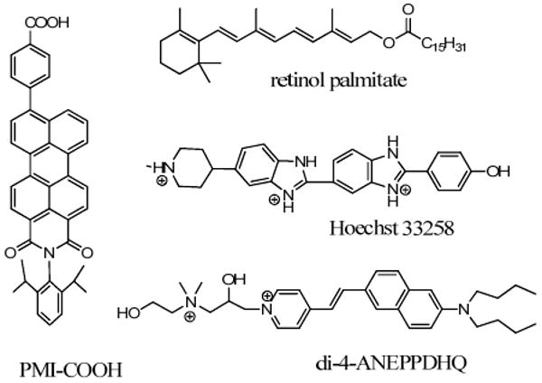
Examples of fluorescent compounds increasing lifetime in higher viscosity media.

Polarity

In addition to temperature and viscosity, the fluorescence lifetime also depends on the polarity of the media. The classical example of this lifetime solvatochromism is the increase of fluorescence lifetime of the dyes after binding to albumin: 1-anilino-8-naphtalene sulfonate,¹⁰⁸ squaraines,^109,110 Rhodamine 800,¹¹¹ cyanines,¹¹² etc, all increase their lifetimes, sometimes by an order of magnitude compared to the free state, if bound to albumin. Lifetime solvatochromism is less understood¹¹³ than its steady-state counterpart.^114,115 In steady state solvatochromism, the absolute change of dipole moment value is the major reason for spectral shifts, while conformational stability of the excited molecule is the most critical factor affecting fluorescence lifetime. Recently, it was shown that NIR polymethine dyes lacking a dipole moment and having weak steady-state solvatochromism exhibit strong and predictable lifetime dependence to a solvent polarity function called orientation polarizability (Fig. 14),⁵¹ derived from a combination of solvent dielectric constant and refraction index.^3,116,117 This finding established the foundation for developing lifetime polarity probes, which we suggest should be named “solvatochronostic” dyes, from Greek Χρόνός (time) and the change in the lifetime associated with these dyes as “solvatochronism”.

Figure 14.

Structures and fluorescence lifetime of cyanine probes vs. solvent orientation polarizability. 1 – water, 2 – methanol, 3 – ethanol, 4 – acetone, 5 – DMSO, 6 – methylene chloride, 7 – chloroform. Adapted from Ref. 51 Copyright 2007 Elsevier.

4.1.2 Excited state electron and proton transfer

Environmental factors, such as temperature, viscosity, and polarity affect fluorescence lifetime via induced conformational changes. Alternatively, fluorescence lifetime could be also affected by reversible changes in electron distribution occurring in the excited state. These changes are strongly structurally related and less susceptible to environmental factors. The most important processes from this class are excited state charge transfers such as electron transfer (ESET) and proton transfer (ESPT) and intersystem crossings (Fig. 1 and 15). The manipulation of these processes gives rise to the manufacturing of conductive polymers, fluorescence based metal sensors, pH probes, black quenchers, and long lived fluorophores, many of which are actively used in fluorescence lifetime imaging.

Figure 15.

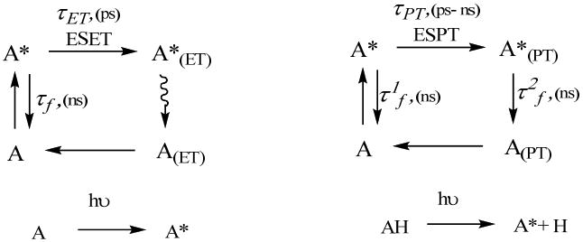
Schematics and timescale of the excited state electron transfer.

In systems with ESET, the electrons in the excited state travel from the electron rich donor to the electron acceptor upon photoexcitation. In internal ESET, most common in fluorescence, this effect is observed within the same molecule when the donor is in close proximity to the acceptor (1-3 bonds). ESET occurs on a very fast scale, typically on the order of subpicoseconds,¹¹⁸ resulting in a non-fluorescent product, which relaxes non-radiatively to the ground state (Fig. 15). This fast relaxation process lowers the fluorescence lifetime of the quenched molecule and does not contribute to the measurable part of fluorescence lifetime defined as an average from the two emissive states (Eq. 7) due to negligible fractional contribution from the A*_(ET).

Molecules capable of undergoing an electron transfer possess strong electron donating and, occasionally, electron withdrawing groups.¹¹⁹ The electron donating functionalities are composed almost exclusively from amines with the quenching strength order of tertiary > secondary > primary, which, incidentally, might explain the absence of fluorescence and very short (∼ 4.7 ps) lifetime of mauveine³¹ and the bright fluorescence of Magdala red. Among electron withdrawing groups, only a nitro group has been used successfully in quenchers. The exceptions are however numerous and a number of molecules with electron donor or electron withdrawing groups affect fluorescence only partially. For example, tetranitrofluorescein (Fig. 16) has a lifetime of 2.3 ns¹²⁰ compared to ∼4.0 ns for fluorescein.

Figure 16.

Typical ESET molecules with electron donating tertiary amines and electron withdrawing nitrogroups.¹²⁰,⁵⁴²,⁵⁴³

A large group of molecules exhibiting ESET utilize d-orbital and f-orbital of metals, such as Ru(II)-, Eu(III)-, and Nb(III)-based probes. This mechanism, although based on the same principle as ESET, is categorized as either ligand-to-metal or metal-to-ligand charge transfers (LMCT and MLCT). Due to their extremely long lifetime emission in the microsecond range, they are widely utilized in applications such as time-gated microscopy and in vitro and in vivo oxygen sensing (see Section 6.4 for further discussion).

In ESPT systems, the protons in the excited state depart or join the molecule at rates different from the ground state. ESPT is easy to recognize from the steady-state spectra: the absorbance is generally similar to the parent chromophore, but fluorescence is significantly compromised. ESPT is also a fast process compared to fluorescence emission, with reported values ranging from fractions of picoseconds to tens of picoseconds.^95,121,122 Here, the intramolecular proton transfer is faster than intermolecular. The rate of proton transfer is environmentally dependent,¹²³ and in the nanocavities of cyclodextrin or in emulsion, this becomes much slower, reaching nanoseconds for the reaction to proceed.^124-126 Often, the product and the starting materials have distinct fluorescence lifetimes. For example, a pH-sensitive fluorescent imidazole with an initial lifetime of 0.3 ns after ESPT gives a deprotonated fluorophore with a fluorescence lifetime of 0.5 ns (Fig. 17).¹²⁷ Such pH lifetime sensitivity within the same spectral range (550-600 nm) can be potentially utilized in lifetime-based pH imaging.

Figure 17.

Deprotonated fluorescent imidazole in the excited state is more acidic than in the ground state and has a shorter fluorescent lifetime than the protonated imidazolium.¹²⁷

4.1.3 Inter system crossing

Intersystem crossing from a singlet to a triplet state substantially affects the fluorescence lifetime of the molecule: the singlet lifetime becomes shorter and a new component corresponding to the triplet state on the order of microseconds appears. The mechanism of intersystem crossing from the S to T state is similar to the charge transfer from one set of orbitals to another¹²⁸ and occurs via spin-orbit coupling of a singlet state to the closely related vibronic levels of T states (e.g. upper levels of T₁), as schematically shown in Fig. 1.

In the absence of other non-radiative processes, the lifetime of the singlet state τ_S and the lifetime of the triplet state τ_T are given in Eq. 15. For typical organic fluorophores composed of light atoms (C, N, O, H, etc.), the rate constant k_ST is relatively small compared to the rate constant of fluorescence k_f(k_st ≪ k_f) and stable toward structural modifications. For example, differently substituted rhodamines retain the same S→T rate constants (∼5.3 × 10⁶ sec^-1)¹²⁹ compared to the rate constant of fluorescence (k_f ∼5.1 × 10¹⁰ sec^-1).¹³⁰ However, when the fluorophore is substituted with heavy atoms such as Br or I, the k_ST increases dramatically, reaching 10¹⁰ sec^-1 for iodo-substituted molecules such as Rose Bengal (Fig. 6) and leading to strong phosphorescence with phosphorescence lifetime of ∼100 μs.¹³¹ Consequently, the fluorescence lifetime drops from nanoseconds to picoseconds (89 ps).¹³² Many lifetime probes utilizing the heavy-atom effect belong to a class of metalloporphyrins considered in the Section 6.4.

$${\tau }_S=\frac{1}{k_f+k_{\mathit{\text{ST}}}};{\tau }_T=\frac{1}{k_f+k_{\mathit{\text{TS}}}};$$ Eq. 15

where k_ST is rate constant of the intersystem crossing from S1 to T1.

4.2 External quenching mechanism

4.2.1 Förster Resonance Energy Transfer (FRET)

Förster Resonance Energy Transfer (FRET), named after Theodor Förster who laid a mathematical foundation of this process,¹³³ is an energy transfer mechanism between two chromophores such as traditional organic dyes, fluorescent proteins, lanthanides, quantum dots,^134,135 fullerenes, carbon nanotubes¹³⁶ and their combinations.¹³⁷ FRET is used by a family of techniques that includes normal and confocal FRET, multiphoton FRET, photobleaching FRET, single-molecule detection FRET, bioluminescence energy transfer (BRET), correlation FRET spectroscopy, anisotropy/polarization FRET,^138,139 and lifetime FRET, with significant overlap among them. For a long time, the primary goal of FRET based methods was to determine the distance between interacting molecules, mostly proteins, by monitoring changes in fluorescence intensity of either the donor or the acceptor molecule. Later, with the development of fluorescence lifetime imaging measurement, FRET became a powerful method to study structures, interactions, and functional events between molecules in cells and small animals.^140,141 FRET causes quenching of the donor fluorescence but a large part of the energy is emitted via the acceptor. In this regard, FRET has the attributes of both energy transfer and quenching mechanisms. For a FRET effect to occur, the presence of an acceptor with an appropriate set of orbitals and energies close to or lower than that of the excited state of the donor is required (Fig. 18). This implies that the emission spectra of the donor must overlap with the absorption spectra of the acceptor. This energy transfer could be directly measured using fluorescence lifetime of the molecular construct according to Eq. 16 if the lifetime of the fluorophore τ_d is known. During FRET, the lifetime of the donor decreases due to the presence of non-radiative processes (Eq. 5, k_nr = k_FRET) and the lifetime of the acceptor remains intact. This statement is only valid if no reverse energy transfer occurs but in reality, back-FRET does occur if the acceptor is a fluorophore with sufficiently long S1 lifetime and part of its emission spectra overlaps with the absorption spectra of the donor.¹⁴² This condition is often achieved if two identical fluorophores form a FRET pair (homoFRET), in which case the overall lifetime decreases if the two fluorophores are close.

Figure 18.

Diagram of FRET. Upon excitation by the photon, the electron of the donor is promoted to the excited state (1) followed by the energy transfer to the acceptor excited orbital (2), simultaneous return of the excited electron back to the ground state (3), and excitation of an acceptor (3).

$$E_t=1-\frac{{\tau }_{\mathit{\text{da}}}}{{\tau }_d},$$ Eq. 16

where τ_da is the fluorescence lifetime of the donor in the presence of the acceptor and τ_d is the lifetime of the donor without the acceptor

The energy transfer E_t between the fluorophore and the acceptor, as well as the fluorescence lifetime of the donor in the presence of an acceptor, can be expressed via the distance r between them using Förster equations (Eq. 17 and Eq. 18). The fluorescence lifetime of the donor is directly proportional to the distance between the donor and the acceptor, as illustrated in Fig. 18. At distance R₀, known as the Förster radius, and under the measurement conditions postulated in Eq. 19, the fluorescence lifetime is exactly half of the lifetime of the donor alone. At this point, the lifetime is most sensitive to alterations in the distance.

$$E_t=\frac{R_0^6}{R_0^6+r^6}\times 100$$ Eq. 17

$${\tau }_{\mathit{\text{da}}}={\tau }_d\frac{r^6}{r^6+R_0^6}$$ Eq. 18

r - distance between two fluorophores, R₀ – Förster radius where half of the energy is transferred

$$\begin{array}{c}{R}_0=0.211{(k^2{n}^{-4}{\Phi }_{D}J(\lambda ))}^{1/6},\mathring{\mathrm{A}}\\ \text{and}\\ J(\lambda )={\int }_0^{\infty }{F}_D(\lambda ){\epsilon }_A(\lambda ){\lambda }^{4}d\lambda ,{\text{M}}^{-1}{\text{cm}}^{-1}{\text{nm}}^4\end{array}$$ Eq. 19

where n – refraction index is typically assumed to be 1.4 for biomolecules in aqueous solutions but may vary from 1.33 to 1.6 for biological media, k²- orientation factor, equal to 2/3 for randomly distributed fluorophores, but could be within the range 0-4 (see the discussion in the text), Φ_D- quantum yield of the donor, J(λ)- spectral overlap integral, where λ -wavelength (nm); F_D(λ) – fluorescence intensity normalized to emission intensity at λ (dimensionless); ε_A(λ) –molar absorptivity of the acceptor at given λ (M^-1 cm^-1).

The use of Eq. 18 requires knowledge of the fluorescence lifetime of the donor in the absence of the acceptor (τ_d). An accurate value of τ_d might be difficult to attain because the lifetime of the donor in a free form could be different from that of the donor-acceptor molecular system. An efficient and practical method to measure τ_d is through selective acceptor photobleaching,^143,144 where the acceptor is selectively destroyed by illuminating at the acceptor absorption spectrum. The FRET efficiency using this method can be readily calculated from the relative increase in the donor emission intensity and lifetime after acceptor photobleaching. Acceptor photobleaching can be carried out with high selectivity without affecting the donor if the excitation is performed near the red-edge of the acceptor excitation spectrum.⁵⁰

The major uncertain parameter in Eq. 19 is the “infamous”¹⁴⁵ orientation factor k² which reflects the relative orientation of two oscillating dipoles (Fig. 19B) and is defined according to Eq. 22. The orientation factor has been known for being notoriously difficult to measure and the uncertainty in its value might cause a large error in distance measurement. The problem arises because both dipoles are in a dynamic process, hence the mutual orientation is constantly changing. Because of this dynamic state, the orientation factor seldom has a single value but rather resides within a range. Typically, it spans from 0 for a perpendicular orientation (no energy transfer) to 4.0 for parallel or anti-parallel orientation (non-restricted energy transfer). For completely random movement, the range narrows down to a single value with k²=2/3,¹⁴⁶ which appears in most publications. For practical applications, it has been suggested to evaluate the rotational freedom of the donor and the acceptor by measuring their anisotropies. If the anisotropy values are smaller than 0.2 (on a scale from 0 to 0.4), then the fluorophore is considered to be undergoing random rotation^147-149 and the value of 2/3 can be safely applied.¹⁵⁰ For a system with non-random orientation, several mathematical models defining the ranges of k² have been developed.^146,151-155 For example, the absolute limiting values for k² were defined as 0.14 and 1.19, which corresponds to an uncertainty of ±14% for measuring intramolecular distance.¹⁵³ With the development of computational methods, k² has been evaluated using Monte Carlo¹⁵⁶ and molecular dynamic simulations.^92,157-160

Figure 19.

A. Dependence of the fluorescence lifetime of a typical DA pair as a function of the distance in Förster energy transfer mechanism and Dexter electron transfer. B. Dipole vectors and their angles for the donor (D) in the excited state and the acceptor (A) in the ground state (from ¹⁴⁶). C. Fluorescence lifetime changes as a function of orientation factor (k²), derived from Eq. 22.

$$k^2={(\text{cos}\alpha -3\text{cos}\beta \text{cos}\gamma )}^2$$ Eq. 20

where k² is the orientation factor, α is the angle between dipoles, and α and γ are the angles between the dipoles and the line connecting their origin of the dipoles.

It is possible to show fluorescence lifetime of the donor in the presence of the acceptor τ_da is inversely proportional to the orientation factor (Eq. 21; rearranged from ref.140). Graphically, this dependence is illustrated in Fig. 19C, where the largest change in fluorescence lifetime occurs at distances close to the Förster radius. This dependence presents an interesting rationale for developing new orientation-sensitive molecular probes, where changes in orientation will affect fluorescence lifetime. Such orientation sensitive probes could potentially open up new possibilities in studying molecular interactions and donor-acceptor microenvironments from time resolved studies.

$${\tau }_{\mathit{\text{da}}}={\tau }_d\frac{r^6}{r^6+C{k}^2}$$ Eq. 21

Where C – is the constant for the given donor-acceptor pair accommodating overlap integral, Förster radius, quantum yield and refractive index.

As noted above, for FRET to occur, the donor and the acceptor have to be within certain distance from each other. In one of the major FRET applications – investigating the interaction between proteins – all of the donors may not interact with the acceptors. This condition leads to two populations of donors with distinct fluorescence lifetimes: one with the donor lifetime corresponding to τ_d and another with a shorter lifetime τ_da caused by the quenching process. Both donor populations can be resolved by lifetime-based FRET techniques using double exponential decay analysis.

4.2.2 Dexter electron transfer

At distances significantly shorter than the Förster radius, the donor and acceptor experience an overlap of their wavefunctions, resulting in a channel transporting an electron from the donor in the excited state to the ground state acceptor (Fig. 20). These short-range processes are of fundamental importance in a variety of molecular electronic devices and biological systems such as photosynthesis and DNA analysis. Although FRET and electron transfer (ET) are different processes, they share common features, such as spectral overlap. A theory for ET was developed by Dexter¹⁶¹ in response to the need for Förster energy transfer to accommodate shorter distances between the molecules. Initially, the theory was developed for solid state, where the molecules are closely packed and later it was modified to bichromic molecules in a manner similar to the Förster donor-acceptor paradigm.^162,163 According to Dexter theory, the rate constant by ET is expected to decrease exponentially as the distance of the electron from the excited donor and the ground state acceptor is increased (Eq. 22¹⁶⁴). Similar to FRET, the rate of the electron transfer is directly proportional to the spectral overlap and could be written in a form similar to Förster relation. The constants K and L are difficult to measure experimentally and they are normally evaluated from a set of quantum yield - lifetime data using a modified Dexter equation.^162-164

Figure 20.

Dexter electron transfer: In the initial state, the donor and acceptor orbitals are overlapping. Upon excitation by the photon, the electron of the donor is promoted to the excited state (1), followed by the electron transfer to the acceptor excited orbital (2), and back electron transfer from the acceptor in the excited state to donor (3).

The majority of publications describing Dexter mechanism are related to a solution of a classic problem in excited-state chemistry to distinguish between electron and energy transfer.^165-169 Computational approaches in distinguishing these processes have been recently reviewed.¹⁷⁰ It has generally been concluded that the Dexter electron transfer can only be observed at distances less than 10-15 Å as required by orbital overlap.^171,172 However, several systems, especially those based on DNA-organometallic intercalating complexes, have shown possible calculations of Dexter's ET at up to 40 Å donor-acceptor separation.^173,174 A graphical comparison of Förster and Dexter distance dependent interaction is shown in Fig. 19A.

$$\begin{array}{c}{k}_{\mathit{\text{ET}}}=\frac{2\pi }{\hslash }\mathit{\text{KJ}}(\lambda )e^{(-2R_{\mathit{\text{da}}}/l)}\\ J(\lambda )={\int }_0^{\infty }{F}_d(\lambda ){\epsilon }_a(\lambda )d\lambda \end{array}$$ Eq. 22

Rate constant k_ET for Dexter electron transfer (ET)¹⁶⁴: l is the average orbital radius involved in initial (D*A) and final (DA*) wavefunctions, K is a specific orbital interaction and is a constant which, unlike R₀, is unrelated to any known experimental parameter, J is spectral overlap, where molar absorptivity of the acceptor ε_a and fluorescence intensity of the donor F_d are normalized to unity, R_da is the donor-acceptor distance. Note that the overlap integral is different from the Förster equation.

Recently, a new class of compounds occupying the intermediate position between FRET and ET based on alkynylyne bonds connecting two fluorophores has been reported from different groups (Fig. 21). Alkynyl groups are known to be an effective bridge for energy transfer processes^175-179 and have been found to be highly effective in facilitating through-bond electron transfer channels with a low attenuation factor (0.04 per Å).^180,181 Although such constructs have not yet been applied for lifetime imaging, they have some promising characteristics as unique labels.

Figure 21.

ET constructs with alkynyl bonds¹⁶⁰,¹⁷⁵,⁵⁴⁴

4.2.3 Dynamic quenching

The process of quenching where the excited fluorescent molecule loses its energy non-radiatively via collision with other molecules is called dynamic quenching. In this process, the energy from the excited molecule A* is transferred to the quencher Q with a rate constant k_q according to the reaction in Eq. 20. The molecules decrease their fluorescence lifetime as a result of multiple processes at the moment of collision such as the formation of metastable complexes, resonance energy transfer, electron transfer, etc. Due to lifetime sensitivity, dynamic quenching and probes based on this principle play an important role in lifetime imaging for measuring oxygen and other analytes.

To explain dynamic quenching of a fluorophore, the Stern-Volmer equation is commonly utilized (Eq. 23). In its original form, the equation describes the change in fluorescence intensity with (F) and without (F₀) the quencher.

$$\begin{array}{l}{A}^{\ast }+Q\stackrel{k_q}{\to }A+Q^{\ast }\\ \frac{F}{F_o}=1+k_q{\tau }_0[Q]\end{array}$$ Eq. 23

Where τ₀ is the fluorescence lifetime without the quencher, Q is the concentration of the quencher and k_q is the rate constant of quenching

Eq. 23 can be re-written in a form more suitable for lifetime imaging (Eq. 24)

$$\tau =\frac{{\tau }_0}{1+k_q{\tau }_0[Q]}$$ Eq. 24

For a diffusion controlled reaction, the rate constant k_q can be replaced by the diffusion rate constant rate k_d. In the case of a very effective reaction, as in cases where the reaction occurs immediately after the quencher Q and A* come into contact, a familiar Smoluchowski theoretical expression can be used (Eq. 25).¹⁸²

$$k_q\cong k_d=4\pi r_{\mathit{\text{AQ}}}{D}_{\mathit{\text{AQ}}}$$ Eq. 25

where k_d is the rate at which reactants diffuse together, r_AQ is the distance at which reaction occurs, and D_AQ is the sum of diffusion coefficients for the reactants

The diffusion rate constant described by this equation can be determined by using the general Stokes-Einstein equation (Eq. 26)

$$D_i=\frac{\mathit{\text{kT}}}{6\pi \eta r_i}$$ Eq. 26

Where D_i is the diffusion coefficient of the participating molecules, r_i is their radii, and η is viscosity

Assuming that diffusion coefficients for the quencher and the excited molecules are equivalent and their radii of action are the same, then:

$$\begin{array}{c}{D}_{\mathit{\text{AQ}}}=D_A+D_q=2D_i\\ r_{\mathit{\text{AQ}}}=r_A+r_q=2r_i\end{array}$$ Eq. 27

Combining and rearranging. Eq. 25 - Eq. 27 and incorporating the probability function of the quenching process p, which is characteristic of the quencher gives Eq. 28.

$$k_q=\frac{8r_{\mathit{\text{AQ}}}T}{3\eta }\times \frac{N_A}{1000}\times p$$ Eq. 28

where N_A/1000 is a conversion factor to molecules per cm³, ^3,183 and p is the probability of the quenching process

Certain small molecules like iodine and oxygen have a high probability of quenching p close to unity. Fluorescence decay functions produced by such quenchers are monoexponential and have been used for a variety of applications, such as for convenient preparation of mono-exponential decay standards with variable lifetimes,¹⁸⁴ in the manufacture of microfluidic tools,^185,186 and measuring oxygen concentration. The decrease of fluorescence lifetime is proportional to oxygen concentration [Q] (Eq. 24) and by measuring the change in fluorescence lifetime, oxygen concentration or partial oxygen pressure can be evaluated.

4.3 Other processes affecting fluorescence lifetime measurements

4.3.1 Photon reabsorption

One of the major advantages of fluorescence lifetime imaging is the independence of the lifetime from concentration. This statement is however only valid for a certain range of concentration in which fluorophores do not interact either chemically or photonically. It is also essential that a minimum concentration threshold be attained to provide sufficient fluorescent signal for lifetime measurement. At high concentrations, fluorescence lifetime can increase due to a trivial process of photon re-absorption, and at even higher concentrations it may start decreasing because of other effects such as resonance energy transfer between two closely located fluorophores or formation of non-fluorescent dimers and higher aggregates. The typical appearance of the measured fluorescence lifetime vs. concentration of a fluorophore is depicted in Fig. 22.¹⁸⁷ In a reabsorption process, the fluorescence lifetime remains unchanged and only the measureable lifetime value is affected, often significantly. For example, in highly concentrated solution, the lifetime of Rhodamine 6G changes from ∼4 ns to ∼11 ns.¹⁸⁷ Similarly, DBPI increases from 3.7 ns to 8.5 ns.¹⁸⁸

Figure 22.

Structures of Rhodamine 6G and DBPI used in reabsorption studies. For DBPI the probability of self-re-absorption for concentrations 1 uM to 1 mM is 0 - 0.56, φ = 0.98 resulting in the lifetime range from 3.7 to 8.52 ns.¹⁸⁸ Chart: Fluorescence lifetime of Rhodamine 6G in methanol (molecular fluorescence lifetime is ∼ 4 ns) as a function of the concentration of the dye: (◊) measured lifetime, (■) measured lifetime corrected for self-absorption. Reprinted from Ref. 187 Copyright 1977 American Chemical Society.

In these situations, the measurable (apparent) fluorescence lifetime τ_ra can be expressed as the probability of reabsorption (Eq. 29)¹⁸⁹, which depends on the overlap between the emission and absorption spectra, as well as the concentration of the sample. Thus the influence on the measured lifetimes depends on the thickness of the sample and on the optical configuration of the experiment. The reabsorption process can affect the outcome of fluorescence lifetime imaging even in biological systems, where low concentrations are typically used.¹⁹⁰

$${\tau }_{\mathit{\text{ra}}}=\frac{\tau }{1-a\Phi },a=f(J,c)$$ Eq. 29

where a is the probability of reabsorption as a function of the overlap between emission and absortion (J) spectra and concentration of the fluorophore (c), Φ – quantum yield

4.3.2 Excimers

A number of aromatic molecules and their derivatives experience an excimer (excited dimer) formation when an excited molecule associates with the same molecule in the ground state. The characteristic feature of an excimer is an emission spectrum distinct from the monomer with the retention of the same absorption spectrum. The excimer forming pyrene (Fig. 11) and its derivatives have been used extensively in fluorescence steady-state and dynamic imaging.^191-193 The importance of pyrene in steady-state imaging lies in its large spectral shift from the monomer (400 nm) to the excimer (485 nm) state. For lifetime imaging, its utility is based on its remarkably long fluorescence lifetime (monomeric 680 ns and excimeric 90 ns¹⁹⁴). Such a long lifetime is used in biological systems to completely eliminate autofluorescence background, which is on the scale of 5-7 ns for cell studies.^195,196 In addition, due to their long lifetimes, pyrenes and their excimers are extremely sensitive to external factors such as the presence of oxygen,^197,198 free radicals,¹⁹⁹ and neurotoxins²⁰⁰ and they are utilized extensively as reporters for DNA hybridizations,²⁰¹ RNA recognition,¹⁹⁶ and actin assembly.²⁰²

For example, the long lifetime of pyrene excimers (∼ 40 ns) compared to cellular extracts (∼ 7 ns) has been utilized to detect specific mRNA complementary pyrene bearing probes (Fig. 23). This method allowed selective detection of the mRNA via excimers using time-resolved emission spectra and could be used in conjunction with time gated fluorescence mapping¹⁹⁶ to completely eliminate non-excimeric signals.

Figure 23.

Pyrene probes after hybridizing with target (blue) form an excimer with long fluorescence lifetime.¹⁹⁶

In this review of photophysical processes affecting fluorescence lifetime, we selected only those which are currently and frequently utilized in lifetime imaging. None of these processes exists separately and the change in fluorescence lifetime is induced by a variety of factors. Some important lifetime altering processes induced by the presence of paramagnetic metals, spin-orbit couplings, delayed fluorescence, and many others were omitted from this review due to the lack of their applications in lifetime biological imaging. However, with the rising interest in fluorescence lifetime imaging applications, these and many other photophysical processes will certainly become part of the arsenal for molecular imaging of normal and abnormal cells and tissues in the near future.

5 Autofluorescence

It was noted hundreds of years ago that some biological substances possess intrinsic fluorescence, known today as autofluorescence. The earliest report of autofluorescence was apparently published in the 16th century when the blue opalescence of an extract from a Mexican wood known in Europe as Lignum nephriticum was observed.²⁰³ The fluorescence origin of the opalescence was confirmed only very recently and was found to be the product of flavonoid oxidation.²⁰⁴ Other naturally occurring fluorophores, such as the familiar quinine and chlorophyll and the exotic escubin and curcumin were discovered in the 19^th century.²⁰⁵ With the invention of the fluorescence microscope in 1908, autofluorescence studies of cells and tissue became possible.^206,207 Since then, a great number of fluorescent materials emitting in the range from 250 nm to nearly 800 nm have been found, isolated, and re-synthesized. The optical properties of some of these compounds, including lifetimes, have been described (Table 4).

Table 4.

Representative endogenous fluorophores responsible for autofluorescence in proteins, microorganisms, plants and animals.

Fluorophore	Excitation, nm	Emission, nm	Lifetime, ns	ref
phenylalanine	258 (max) 240-270	280 (max)	7.5	31
tyrosine	275 (max) 250-290	300 (max)	2.5	32
tryptophan	280 (max) 250-310	350 (max)	3.03	33
NAD(P)H free	300-380	450-500	0.3	34
NAD(P)H protein	300-380	450-500	2.0-2.3	34
FAD	420-500	520-570	2.91	34, 35
FAD protein bound	420-500	weak in 520-570	<0.01	219
flavin mononucleotide (FMN)	420-500	520-570	4.27-4.67	35, 36
riboflavin	420-500	520-570	4.12	35
protoporphyrin IX	400-450	635,710	up to 15	34, 37
hemoglobin	400-600	non-fluorescent	n/a
melanin	300-800	440,520, 575	0.1/1.9/8	34
collagen	280-350	370-440	≤ 5.3	34, 38
elastin	300-370	420-460	≤ 2.3	34, 38
lipofuscin	340-395	540,430-460	1.34	39
chlorophyll a in leaves PS II	430, 662	650-700, 710-740	0.17-3 ns	40, 41
chlorophyll b in plants	453, 642	non-fluorescent	n/a
lignin	240-320	360	1.27	42

The importance of autofluorescence for studying cells and tissues lies mostly in their potential for diagnostic applications²⁰⁸ and as a research tool for understanding the underlying mechanisms of molecular interactions and signaling processes under their native conditions. The most important autofluorophores in cells and tissues are amino acids, the essential building blocks of proteins and enzymes, NADH and FAD which regulate cell metabolism, porphyrins as a side product in mammals and crucial light absorbing element in plants, structural proteins responsible for rigidity and flexibility of tissues and organs, and fluorescent pigments, markers of many age-related pathologies. Herein, we will provide a brief review of their fluorescent properties with an emphasis on fluorescence lifetime applications and, particularly, autofluorescence lifetime imaging.

Autofluorescence lifetime imaging is an attractive modality because it does not require complicated staining procedures in vitro or administration of exogenous molecular reagent in vivo. However, a number of challenges associated with the complex nature of autofluorescence including difficulties in interpretation of images, among others, limit its broad applications. To illustrate the complexity of time-resolved imaging, consider a typical fluorescence lifetime image consisting of lifetime values recorded for each pixel. Due to the presence of multiple fluorophores with distinct lifetimes, the overall decay function for any given pixel will be inherently multiexponential with each component reflecting a fractional contribution of an individual fluorophore. Furthermore, each individual autofluorophore typically exists in a number of states with its own characteristic lifetime. For example, the fluorescence lifetime of tryptophan in proteins varies by a factor of 100, depending on the environment and position relative to other fluorophores.^209,210 To simplify imaging, a careful selection of excitation and emission conditions to eliminate unwanted fluorescence from other autofluorescent species is commonly used. A number of spectral lifetime instruments that simultaneously collects fluorescence lifetime data from separate spectral channels have also been developed.^4,211-216 With the development of supercontinuous lasers and simultaneous excitation of multiple endogenous fluorophores, the separation of the signals from different autofluorophores has become less problematic.²¹⁷

To facilitate image interpretation, multiexponential decay analysis is often used. This analysis delivers several decay components with distinct fluorescent lifetimes and amplitudes. Mapping of these parameters separately allows the differentiation of two or more fluorophores or fluorophores with different conformations.^218-221 Such a method allows differentiation and monitoring the alteration of two fluorophores, instead of using an average value. Alternative and often complementary approaches in dealing with the complexity of multiexponential images include stretched exponential,^218,222,223 global fitting algorithm,^224,225 Laguerre deconvolution method,^226,227 or the phasor analysis method.^228-230 These methods have been recently reviewed elsewhere.²³¹ The fluorescent lifetime properties of representative autofluorophores are summarized below.

Amino acids

Only three amino acids are fluorescent in the range where conventional fluorescence instrumentation could be utilized (>300 nm, higher excitation energy might destroy biological samples): phenylalanine, tyrosine, and tryptophan (Fig. 24). Most of the amino acids useful for fluorescence lifetime imaging of cells are not present in a free form but are seen mostly in proteins with an occurrence frequency of 3.6:3:1 ratio for phenylalanine, tyrosine, and tryptophan, respectively.²³² Out of these amino acids, tryptophan is more useful for lifetime imaging because of its relatively attractive spectral features in 340 - 380 nm range. Tryptophan, with the high molar absorptivity (5500 M^-1 cm^-1)²³³ and moderate quantum yield (Φ=0.13),²³⁴ dominates the lifetime map (mean average ∼ 3 ns) in the absence of other (exogenous) strong fluorophores in that range. The fluorescence of phenylalanine suffers from poor quantum yield (Φ =0.024)²³⁴ and low molar absorptivity (150 M^-1 cm^-1).²³³ Therefore, despite its long fluorescence lifetime of 7.5 ns, phenylalanine does not contribute to the overall autofluorescence lifetime. Similarly, the molar absorptivity of tyrosine is also low (1200 M^-1 cm^-1)²³³ with negligible weak emission at 350 nm.

Figure 24.

Structures of fluorescent amino acids and fluorescence average lifetime image of SiHa cells. Ex. 600 nm, em. 340-360 nm. Reprinted from Ref. 217 Copyright 2009 Optical Society of America.

Until recently, near-UV fluorescence lifetime imaging was not explored, partly because of the lack of appropriate instrumentation. With the development of novel imaging systems,²³⁵ especially two-photon spectroscopy and supercontinuous lasers,²¹⁷ the 340-360 nm region might present substantial interest. For example, these studies can take advantage of the high sensitivity of tryptophan fluorescence lifetime to its environment^48,209,210 to characterize cells and cellular compartments. Indeed, time-resolved fluorescence images focusing on tryptophan emission in cells demonstrated a wide range of lifetime values with clear differentiation between different organelles (Fig. 24).

NADH

A reduced form of nicotinamide adenine dinucleotide (NADH) and its phosphate derivative (NADPH) (Fig. 25) are the dominant endogenous fluorophores in cells responsible for green autofluorescence upon excitation above 350 nm. NAD(P)H is involved in cell metabolism, reductive biosynthesis, antioxidation, cell signaling, aging, and regulation of apoptosis. For information on the functions of NAD(P)H and related molecules, interested readers are referred to recent reviews in this area.^236-238

Figure 25.

Structures of NAD, NADH, NADPH, FAD, and FADH₂.

NAD(P)H absorbs at 350 nm and emits at 450 nm.²³⁹ This relatively long emission stems from the reduced form of nicotinamide. The oxidized form NAD+ absorbs at a much shorter wavelength (∼ 260 nm) and does not fluoresce, hence only the reduced form is widely used in fluorescence imaging. The intensity and the lifetime of NAD(P)H strongly depends on the microenvironment. NAD(P)H has a mean fluorescence lifetime of 2.3-3.0 ns when bound to proteins and a short lifetime ∼ 0.3-0.4 ns in free form.^240-242 This decrease is mainly the result of radiationless processes arising from free rotation between the pyridine and amide (see Section 4.1.1), which also explains NADH fluorescence sensitivity to solvent polarity and viscosity.²⁴³ Other mechanisms based on dynamic quenching by the adenine moiety has been suggested as the basis for the observed lifetime differences.²⁴⁴

The distinction in lifetime between a free and protein bound nicotinamide adenine dinucleotide forms the basis of almost all fluorescence lifetime imaging techniques aimed at NADH.^240,245 To avoid oxidation stress on the cells caused by high energy (365 nm) one-photon lifetime imaging, two-photon excitation (700-800 nm) technique with femotosecond Ti-sapphire laser has been proposed.⁶¹ The use of much milder irradiation minimized the modification of cellular redox state and cell morphology. It also allowed nondestructive fluorophore detection with high spatial and temporal resolution. To discriminate between free and protein-bound NAD(P)H, biexponential fluorescence lifetime imaging maps of cellular metabolism are typically generated.²²¹.

Flavins

Flavin adenine dinucleotide (FAD) is a redox cofactor with strong fluorescent properties. Many oxidoreductases, called flavoenzymes or flavoproteins, require FAD as a prosthetic group for electron transport. As with NAD(P)H, flavin exists in several redox configurations.²⁴⁶ The two mostly studied forms are the fully oxidized fluorescent (FAD) and the fully reduced non-fluorescent FADH₂ (Fig. 25). FAD emits at a longer wavelength than NAD(P)H, with only small overlap, allowing for selecting imaging conditions specifically for FAD without spectral contamination from NAD(P)H. In contrast to NAD(P)H, only the non-bound form of FAD is fluorescent and it has a lifetime of 2.3-2.9 ns.^247,248 Protein binding leads to a significant decrease of the lifetime of FAD (<0.1 ns).^247,249 Mechanistic studies of such a dramatic reduction in lifetime is the subject of many research activities and reports suggest that the lifetime decrease is induced by the presence of nearby aromatic residues in protein binding pocket that include tyrosines and tryptophans via ESET.^246,250,251

Porphyrins

The most distinguished members of the porphyrin family are bacteriochlorophylls in phototrophic bacteria, chlorophylls in plants, and heme in red blood cells in mammals (Fig. 27). The reddish-orange fluorescence of porphyrins is probably the longest wavelength among all naturally occurring fluorophores and they can be easily distinguished by a set of appropriate excitation and emission conditions. The majority of the porphyrins emit strongly around 600-800 nm. A noticeable exception is heme, whose fluorescence is completely quenched by the coordinated iron. This is why humans can only blush but not glow! The fluorescence of porphyrins in vivo (in plants and bacteria) is markedly lower than when they are free in solution and the efficiency of emission strongly depends on the light conditions. At low light levels, the fluorescence is almost absent and only appears at high irradiation. This non-linear behavior serves as a protective mechanism, where the excess absorbed light energy is released via emission. This concept has been central in chlorophyll research for the last 80 years starting from the discovery of chlorophyll fluorescence.

Figure 27.

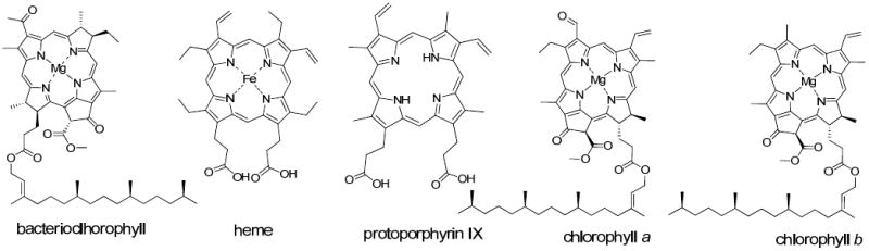
Porphyrins identified in biological tissues.

Fluorescence lifetime has long been recognized as a valuable tool for studying photosynthesis owing to the high lifetime sensitivity of chlorophyll a.^252,253 A historical mini-review focused on the first direct measurements of the lifetime of chlorophyll fluorescence has been published recently.²⁵⁴ Protein complexes known as photosystem I and II (PS I and PS II) play key roles in modulating light utilization in living systems. Under physiological conditions, the fluorescence lifetime of chlorophyll a depends on the activity of PS II reaction centers.²⁵⁵ If the active centers are closed (photosynthetic reactions are OFF), the lifetime increases, reaching ∼3 ns. when the centers are opened (photosynthesis is ON), the lifetime decreases to 170-300 ps. Such change in fluorescence lifetime can be understood from Eq. 5 by substituting the non-radiative rate constant with the rate constant of photosynthesis k_nr = k_PS. The resulting lifetime decreases when the rate of photosynthesis is higher, thus competing with the radiative process. A simplified Jablonski diagram (Fig. 26) illustrates this behavior. Currently, there are two major goals for measuring the fluorescence lifetime of chlorophyll in plants and other organisms. The primary aim is to obtain additional information that will elucidate the mechanistic pathways involved in the numerous aspects of photosynthesis.^256-259 Another application focuses on physiological problems that is largely unexplored. Only few examples of fluorescence lifetime imaging of plants have been reported in literature. These include the assessment of environmental stress, such as the effect of herbicides²⁶⁰ and plant adaptation to excessive light.²⁶¹

Figure 26.

Jablonski diagram of photosynthetic process leading to fluorescence.

In mammals, most red autofluorescence comes either from a diet rich in plants or from porphin producing microorganisms. The presence of endogenous fluorescent porphins in tissues and blood has also been linked with serious pathologies such as cancer, as observed in 1924 by Policard.²⁶² Later studies demonstrated that distinct red fluorescence spots can be seen in oral squamous cell carcinoma.^263-265 The authors observed that this autofluorescence was chromatically different from normal tissue autofluorescence, suggesting different types of porphyrins. Blood analysis of patients presenting with gastric cancer, breast cancer, and Hodgkin's lymphoma also showed enhanced autofluorescence around 630 nm due to the higher concentration of porphyrins.²⁶⁶ Chromatographic analysis of the samples revealed a complex composition of porphyrins in cancer tissues composed of protoporphyrin IX, coproporphyrin, and unidentified components.

Melanin

Melanin is a diverse group of pigments produced by melanocytes and widely present in living organisms including microorganisms, plants, and animals. It is composed from a highly complex mixture of still largely unknown biopolymers derived from tyrosine.²⁶⁷ The most important members of the melanin family are eumelanin (Fig. 28) shows one of the possible components), and pheomelanin (not shown). Eumelanin is a black pigment seen in dark skin, black hairs, eyes, and other organs such as brain. Pheomelanin is a yellow-brown pigment responsible for color of light skin, red hair and blue eyes. The structural difference between the two pigments is discussed in refs.^268,269 A major function of melanin is to protect the body from exposure to UV radiation. This function is achieved through broadband featureless absorbance, low scattering (< 6%), low fluorescence efficiency (< 0.1%) and a highly efficient, ultrafast energy transfer of light energy into heat and chemical reactions.^270,271 The emission decay of melanin is complex, as would be expected from their featureless absorption spectra and the lifetime ranges from picoseconds to almost 8 ns, with an average lifetime of 1.2 ns.^272,273 The chemical and photophysical properties of melanin have been recently reviewed.^274,275

Figure 28.

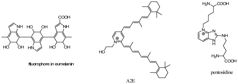
Major components in autofluorescent biological pigments.

In addition to the recognized protective role of melanin as UV absorber and free-radical scavenger, the pigment has many other roles, some of which are not fully understood. Hearing loss has been associated with the absence of melanin,²⁷⁶ loss of neuromelanin, a pigment produced in specific populations of neurons in the brain leads to Parkinson disease,²⁷⁷ and overexposure of melanin to sunlight results in damaged skin cells, causing mutations that lead to skin cancer.²⁷⁸ Due to depletion of the ozone air, skin cancer is expected to become a major health problem of the 21^st century. Application of the fluorescence lifetime of melanin to diagnose and treat skin cancer is described in Section 7.2.

Another interesting application of the fluorescence lifetime of melanin is hair analysis. In contrast to skin, hair is NAD(P)H-free and melanin can be imaged relatively straightforward.²⁷³ Interestingly, blond hair has a much longer lifetime (τ₁=0.34 ns, τ₂ = 2.3 ns) than black hair (τ₁=0.03 ns, τ₂=0.8 ns). The sensitivity of melanin expression and its fluorescence lifetime to a variety of factors such as nutrition, pathologies, and environment renders the fluorescence lifetime in hair a potential target for applications in medicine, pharmaceutics, cosmetics, ecology, and forensics.

Lipofuscin

Lipofuscin is a pale, yellow-brown pigment of molecular weight 6 -7 kDa²⁷⁹ mostly visible in skin as the so-called “age” or “liver” spots. The pigment displays distinct autofluorescence (ex. 440 nm, em. 600 nm) with the first report of its fluorescence in 1911,^207,280 coinciding with the first fluorescence microscopy study of biological tissue. Its structure is, however, still a subject of controversy.²⁸⁰ It is currently believed that the pigment has a pyridinium bis-retinoid skeleton formed from two molecules of vitamin A aldehyde and one molecule of phosphatidylethanolamine.^281,282 The major component, A2E, shown in Fig. 28, and a number of minor components, mainly cis-trans isomers²⁸³ and phosphatidyl analogs,²⁸⁴ have been described and characterized. Lipofuscin forms in the cytoplasm of muscle and nerve cells and has been found in the brain, heart, liver, and other vital organs. This pigment has been implicated in numerous age related diseases such as Alzheimer disease, Parkinson's disease, and heart failure.^279,285-288 Most of the studies associated with lipofuscin autofluorescence have focused on the retina, where the accumulation of lipofuscin in retinal pigment epithelial cells leads to age-related macular degeneration and Stargardt disease.²⁸⁹

By selecting an appropriate set of excitation and emission conditions, lipofuscin can be distinguished from other fluorophores in tissues. In the window of 440-470 nm excitation and 510-700 nm emission, lipofuscin was found to be the brightest endogenous fluorophore in the absence of porphyrins and such conditions have been recently utilized for lipofuscin detection.²¹⁹ Fluorescence lifetime imaging targeting lipofuscin as an earlier marker of eye pathologies has been initiated.^219,290 The decay of lipofuscin in vivo is multiexponential due to a heterogeneous microenvironment consisting of multiple fluorophores with a variety of energy transfers. Several studies have revealed at least two major components with lifetimes of 390 ps and 2.2 ns. The short component has been used to discriminate lipofuscin from other autofluorophores present in the retina such as bound NAD(P)H, melanin, collagen, and elastin.²¹⁹

Collagen and elastin

Collagen and elastin are important slightly fluorescent structural proteins. Collagen is the most abundant protein in animals and its function is to hold different organs in place and together. Elastin is a protein in connective tissue and, as the name implies, allows many tissues in the body to be elastic, that is, to return to their original shape after changing their shape. Elastin is found in organs and tissues undergoing substantial deformations in the life span of the organism, such as skin, blood vessels, lungs, ligaments, bladder, stomach, etc. Both collagen and elastin fluoresce under UV and blue excitation; collagen shows a broad emission up to 500 nm, depending on the excitation wavelength (270-370 nm).²⁹¹ Blue emission of collagen was attributed to tyrosine and dityrosine^292,293 while the yellow-green fluorescence was assigned to pentosidine (Fig. 28), formed in vivo via a Maillard reaction involving pentose lysine and arginine.²⁹⁴ (The same Maillard reaction is actually responsible for bread darkening in toasters and making beer golden brown). Collagen has a longer fluorescence lifetime than elastin, as illustrated in Fig. 29, where the mucosal surface composed of elastin shows an excellent contrast in fluorescence lifetime with collagen rich tissue. In addition to autofluorescence, collagen also produces a SHG signal (see Section 3.3) often used for in vivo nonlinear optical imaging.²⁹⁵

Figure 29.

Fluorescence intensity (left, gray color) and lifetime (right, false color) images of the mucosal surface of a piece of freshly resected normal human stomach (ex. 355 nm). In the top right corner of the piece of tissue, the mucosa was removed to reveal the underlying collagen-rich muscularis propria. The gastric mucosa has a short, homogeneous lifetime on the order of 1000 ps, compared to the longer lifetime of 1600 to 1800 ps of the muscularis propria. Copyright (year) (Name of Publisher) Reprinted from Ref. 461 Copyright 2005 SPIE.

6 Exogenous fluorescent molecular probes and their lifetimes

Autofluorescence lifetime imaging relying on endogenous fluorophores provides rich information detailing the morphological and organizational structure of cell and tissues. In general, autofluorescence lifetime imaging is capable of differentiating one type of tissue from another. This feature is readily used to distinguish healthy from pathologic tissues. However, the method has a number of limitations because of the weak and non-specific fluorescence signals originating from a variety of endogenous fluorophores. For these reasons, exogenous molecular probes have been developed to provide distinct fluorescence lifetime information related to physiological or molecular processes in cells and living organisms.

The advantage of exogenous probes lies in their extreme diversity, ranging from small fluorescent molecules to fluorescent proteins and nanoparticles. They also cover virtually all spectral wavelengths ranging from 250 nm to nearly 1200 nm. Many of these molecular probes have been designed to possess high molar absorptivities, excellent fluorescence efficiency, and a wide range of fluorescence lifetimes from picoseconds to milliseconds. Exogenous molecular probes have been instrumental in determining cellular molecular pathways, revealing mechanisms of cell functions, and elucidating cell interactions in tissues and whole organs. A number of reviews featuring a variety of fluorescent molecular probes in optical imaging have been published.^296-303 Previously, the majority of imaging applications have focused on absorption and fluorescence intensity measurements. With recent advances in time-resolved fluorescence techniques, many of the fluorescence intensity-based studies are being re-visited using fluorescence lifetime measurements. Some of the reports demonstrate that molecular fluorescence lifetime imaging could provide both complementary and unique information about the functional status of a target biomarker in cells and tissue. To further harness the strengths of time-resolved optical imaging, the quest for novel fluorescence lifetime-sensitive molecular probes have increased in recent years.

For efficient fluorescence lifetime imaging with exogenous fluorophores, several factors should be considered, including the use of fluorescent molecular probes (i) with longer lifetimes than their endogenous counterparts; (ii) in spectral window with minimal fluorescence from endogenous fluorophores; (iii) with dominant fluorescence that overwhelm the contribution of autofluorescence to the measured lifetime. In addition molecular probes with long lifetimes are not suitable for the fast scanning devices used in fluorescent lifetime imaging microscopy.

Importantly, the contribution of the molecular probe to the effective average fluorescence lifetime, measured as f_pτ_p, should dominate the contribution from the autofluorescence f_aτ_a (Eq. 30). The contribution of the autofluorescence is a function of excitation/emission conditions. It is much lower in NIR than in UV or visible spectrum of light because the majority of endogenous fluorophores have negligible molar absorptivities above 700 nm, resulting in a low fractional contribution f_a to the measured lifetime in the NIR region. Below is a summary of the fluorescence lifetime properties of representative exogenous molecular probes that are potential useful for biological lifetime imaging studies.

$$\overline{\tau }=f_p{\tau }_p+f_a{\tau }_a$$ Eq. 30

Where f_p, τ_p –fractional contribution and the average lifetime of the fluorophore; f_a, τ_a –fractional contribution and the average lifetime of the autofluorescence

6.1 Small organic fluorophores

Exogenous dyes, including fluorescent molecular probes, have long been used to enhance the contrast in biological material in a process called “staining”. In fact, tissue staining remains the mainstay of many clinical diagnoses of diseases today. For more than 150 years, small organic dyes with hydrodynamic diameter less than 2 nm have proved to be absolutely essential in cell microscopy, histology, and in vivo imaging. Organic dyes still constitute the majority of fluorescent molecular probes used in biological imaging because of their established chemistry, scalability, and diverse physical, chemical, and biological properties. A variety of water-soluble and functionalized organic dyes for labeling biomolecules has been developed and their application in fluorescence intensity imaging has been reviewed in great details.^297,304-307 The utility of small molecules in lifetime imaging was realized in the mid 1970's with the onset of time-resolved fluorescence microscopy.^308,309 For example, 1-anilino-naphthalene-8-sulfonate was shown to probe cell membrane dynamics due to lifetime sensitivity of the fluorophore to viscosity.³¹⁰ Similarly, other studies demonstrated that a hematoporphyrin-derivative exhibited different decay times in cytosol compared to aqueous solution³¹¹ and a fluorescent quinacrine mustard (Fig. 30) was shown to be a powerful DNA intercalating agent that can be used to map chromatin based on FRET-induced changes in lifetime of the quinacrine molecules.³¹² Since the emergence of fluorescence lifetime as an imaging modality, many commercially available and newly synthesized dyes were tested under different conditions to mimic diverse physiological environments^{51,73,313,314} and to find the most suitable candidates for time-resolved imaging. The fluorescence lifetime of these compounds varies from hundreds of picoseconds for cyanines to hundreds of nanoseconds for pyrenes (Table 5). The measured lifetime for many of these dyes depends on a variety of factors such as viscosity, temperature, solvent, pH, and the presence of fluorescence quenchers.

Table 5.

Fluorescence lifetimes of typical probes

Fluorophore	Emission range, nm	Media	Fluorescence lifetime, ns	ref
Acridone	420-500	water	14.2	43
DAPI	420-500	water	2.78	44
Pyrene (excimer)	450-550	ethanol	90	45
Coumarine 6	450-650	ethylene glycole	0.30	46
Fluorescein	450-550	water	4.0	47
Quinacrine mustard	470-530	water	6.0	48
BodipyFL	480-530	water	5.87	49
Alexa 532	500-560	water	2.53	49
NBD	500-560	cell membranes	8.2	50
Rhodamine 123	500-560	PBS in water	3.97	51
	500-560	mitochondria	3.2	51
Alexa 488	500-560	water	4.0	52
Alexa 546	520-560	water	4.06	49
DBPI	520-580	chloroform	3.8	53
Rhodamine 6G	520-600	Methanol	4.0	54
Quinacridone	530-630	water	22.8	43
Rubrene	550-610	methanol	9.9	55
	550-630	methanol	2.5	55
Ethidium bromide	550-650	DNA	20	56
Propidium iodide	560-700	DNA	16.8	57
Rhodamine B	560-630	water	1.74	55
Alexa 647	600-660	water	1.04	58
MR121	600-700	ethanol	1.9	59
Bodipy 630/650	630-680	water	3.89	58
	630-680	ethanol	4.42	58
Cy 5	650-690	water	0.91	58
Aluminum phthalocyanine tetrasulfonate	650-700	aqueous phantoms	5.10	60
Rhodamine 800	650-750	PBS in water	0.68	61
Alexa 750	650-800	water	0.66	49
	660-700	ethanol	1.32	58
ATTO 655	670-760	water	1.87	58
	670-760	ethanol	3.31	58
NIAD-16	670-770	tissue	varies	62
ATTO 680	680-780	water	1.69	58
	680-780	ethanol	3.04	58
DTTCI	750-850	methanol	1.07	63
	750-850	DMSO	1.49	63
Cypate	750-850	methanol	0.46	63
	750-850	DMSO	0.87	63
Indocyanine green	750-850	methanol	0.51	63
	760-860	DMSO	0.97	63
Bacteriochlorophyll	750-850	ethanol	2.18	63
Pyrrolopyrrole cyanine-BF2 (PPC-BF2)	750-850	DMSO	4.02	64
	750-850	albumin/water	3.89	64
Pyrrolopyrrole cyanine-BPh2 (PPC-BPh2)	810-900	DMSO	3.35	64
	810-900	albumin/water	2.95	64

The choice of a dye for a specific lifetime application requires more careful analysis of the potential role of the dye in imaging. Organic dyes in general follow the rule that a higher fluorescence quantum yield correlates with a longer fluorescence lifetime. Thus, molecular probes with higher quantum yields and longer lifetimes are preferable for lifetime studies to provide a good imaging contrast. Structurally, these dyes have a rigid fluorophore structure (Fig. 11) and their long lifetime is ensured by the absence of rotatable bonds in the excited state. Rigid dyes are ideal for FRET studies, where the change in fluorescence lifetime indicates mostly a change in the distance between the donor and the acceptor. In general, rigid dyes lack sensitivity to environmental factors such as viscosity and solvent polarity but they are susceptible to quenchers (i.e. oxygen), which makes them potential lifetime biosensors. To enhance the molecular probe's sensitivity to its environment, rotatable bonds can be appended to rigid dyes (compare Rhodamine B and Rhodamine 101, Fig. 58). Dyes with flexible bonds, such as cyanines and styryls, have shorter fluorescence lifetimes than the rigid analogues and are less sensitive to the detrimental effect of fluorescence quenchers. On one hand, the exceptional sensitivity of these dyes to environmental changes allows their use to identify specific cells, organelles, tissues, and entire organs. On the other hand, the high sensitivity of flexible dyes to the environment makes them less favorable candidates for FRET-related lifetime imaging because of random fluctuations in their lifetimes. For multiplexing applications, where the fluorescence lifetime of individual fluorophores is used to resolve fluorescence signals originated from multiple molecular probes, rigid dyes with fixed fluorescence lifetimes are preferred. Table 6 summarizes the potential applicability of exogenous molecular probes in different types of fluorescence lifetime-based studies. These applications with emphasize on small organic molecules are briefly described below.

Figure 58.

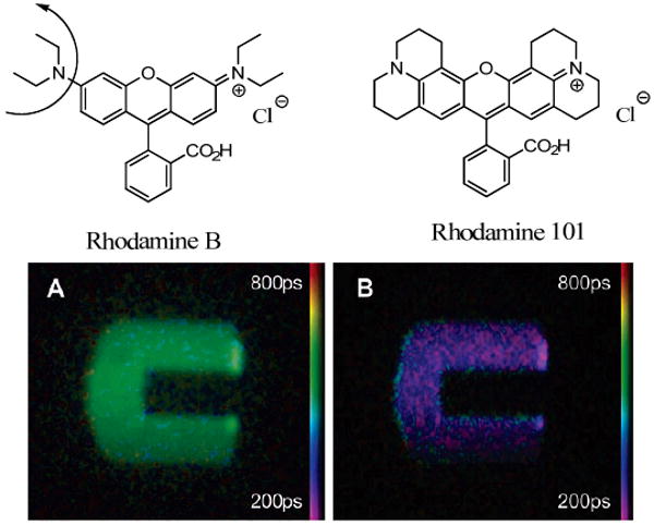
Structures and fluorescence lifetime images of methanolic solutions of Rhodamine B in microchannels. Fluorescence lifetime images at 66 °C (A) and 93 °C (B). Reprinted from Ref. 528 Copyright 2006 American Chemical Society.

Table 6.

Applicability of exogenous probes for different types of lifetime imaging

Fluorophores	Background elimination	Environmental sensitivity	Presence of non FRET quenchers	Presence of FRET acceptors	Lifetime Multiplexing*
Organic molecules with flexible structures	+	+++	+	+	+
Organic molecules with rigid structures	+++	+	++	+++	+++
Fluorescent proteins	+++	+	+	+++	+++
Lanthanides	+++	+	+	+++	+++
Transition metal complexes	++	+++	+++	+	+
Quantum dots	+++	+	+	+	+++

^*Separating fluorescence components by their lifetimes

Background elimination

Autofluorescence might present serious competition in the lifetime imaging with exogenous probes, especially in the visible spectrum of light. For this reason, long fluorescence lifetime dyes with rigid excited state structures are preferable for background elimination. Thus, ethidium bromide, a classic stain for DNA with a long lifetime of ∼ 20 ns when intercalated in the DNA, has been used to completely reject background fluorescence.^315,316 Pyrenes, the dyes with exceptionally long fluorescence lifetime, were used for rapid and sensitive detection of platelet-derived growth factor (PDGF)¹⁹⁵ and mRNA.¹⁹⁶ Alexa-488-labeled antibody with reasonably long lifetimes (∼ 4 ns) were used to differentiate between the extrinsic label and the autofluorescence.³¹⁷ To minimize autofluorescence, imaging in the longer wavelength region using red dyes is preferarred, as exemplified with Rhodamine 800 and MR121 (Fig. 30) in cell studies.³¹⁸ An interesting approach has been proposed to provide a uniform fluorescence lifetime background with τ ∼ 1.0 ns in living cells and the addition of another dye with the longer lifetime such as Hoechst 33342 (Fig. 31) was clearly seen against the low lifetime background.³¹⁹

Figure 31.

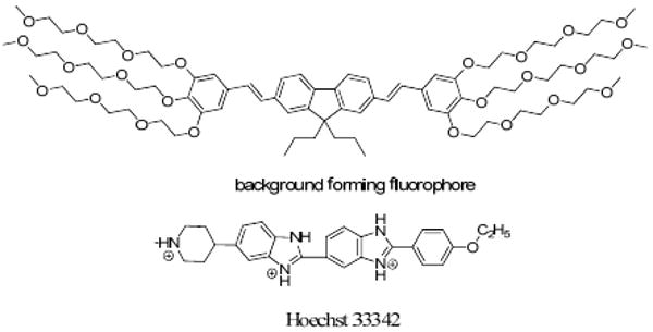
Structures and lifetime background forming compound (τ ∼ 1 ns) and Hoechst 33342 (τ ∼ 1.5 ns) in living CHO cells.³¹⁹

A new method for eliminating background tissue fluorescence is to use NIR fluorescent molecular probes because of the low absorption of light by tissue in this region between 700 and 900 nm. Imaging in the NIR region is also attractive for imaging thick biological specimens and living organisms because of the ability of light to travel longer distances in tissue without attenuation by the absorption process (although light scattering dominates in this NIR window). However, the majority of these dyes have lower fluorescence efficiency (< 25%) and shorter lifetime (< 1.5 ns) than those in the visible region. Molecular probes with short lifetimes in the NIR window do not preclude their use in biological imaging because the low tissue autofluorescence allows the use of a wide range of lifetimes. Thus, the temporal resolution of the imaging instrument becomes the major limiting factor. The short lifetime of NIR fluorescent probes have been attributed to the higher probability of non-radiative relaxation from the excited to the ground state via conical intersection mechanism^320,321 facilitated by a low gap between the orbitals in NIR range. This phenomenon is described by the energy gap law,^322-324 which states that radiationless transitions at longer wavelengths increase due to vibrational overlaps between the ground and excited states and cause a decrease in quantum yield and fluorescence lifetime. Recently, the energy gap law was challenged by new generations of fluorescent dyes based on the pyrrolopyrrole cyanine skeleton.^325,326 The new dyes exhibited high quantum yields (>0.50) in the NIR range, rendering them suitable for in vivo imaging and expanding the fluorescence lifetime window for imaging molecular processes. The first applications of these dyes in vivo lifetime imaging has been demonstrated.⁵²

Environment sensing

Environmentally sensitive molecular probes, such as fluorescent dyes that are sensitive to viscosity and polarity, have been broadly applied in time-resolved imaging in cell studies and tissues to differentiate different organelles, cell types and organs. Thus, Rhodamine 123, a cell-permeable, cationic, green-fluorescent dye with a high affinity to mitochondria has been shown to undergo a noticeable change in fluorescence lifetime from 3.9 ns in solution to 3.2 ns in mitochondria.³²⁷ Similarly, conjugation of Badan (Fig. 30) to a glucose/galactose-binding protein has been used as a glucose sensor. The addition of glucose increased the mean lifetime to a maximum of ∼2 ns.³²⁸ Atto 655, an oxazine dye with a proprietary structure, increased its lifetime from 2.08 ns in free state to 2.85-3.69 ns upon dsDNA intercalating.³²⁹

The nucleic acid dye SYTO 41 has been utilized in two-photon (2P) lifetime imaging of intact mouse carotid arteries.^330,331 The sensitivity of its lifetime to cell type has revealed three distinct layers of wall artery.³³¹ Muscle fibers labeled with a fluorescent ATP analog differentiated myosin from actin (Fig. 32).³³⁰ Cyanine dye Cy5.5, conjugated with chimeric monoclonal antibody rituximab directed against human CD20 antigen which is expressed in the majority of B-cell lymphoid malignancies, showed that the inner part of the tumor has a longer lifetime (1.83-1.93 ns) than the surrounding tissue (1.7-1.75 ns).³³² Cy5.5 attached to antibodies also showed organ-specific lifetime in whole body lifetime imaging in mice: 2.5 ns in gastrointestinal tract, 1.7 ns in primary pancreatic carcinoma and a low fluorescence lifetime of ∼ 1 ns in bladder.^333,334

Figure 32.

Fluorescence lifetime image of a muscle fiber incubated with 39-O-DEAC-pda-ATP. The fiber has a sarcomere length of 2.41 mm (myosin filament overlap 90% with actin). Reprinted from Ref. 330 Copyright 2007 Elsevier.

A novel fluorescence lifetime probe BMVC (Fig. 30) possesses high sensitivity to guanine rich four-stranded structures of DNA known as G-quadruplex.³³⁵ The fluorescence lifetime of BMVC dye in G-quadruplex was shown to be 1.9 ns, substantially higher than in a double stranded DNA (∼1.5 ns), allowing for discrimination between the two forms of DNA.

NIR fluorescent dyes have been used as environmental-sensitive molecular probes for in vivo imaging. Of these dyes, the cyanine family is extensively utilized in vivo imaging.^336-339 Most of the cyanine dyes currently used in biological imaging have relatively flexible fluorophore structures. In the previous sections, we explained that this feature bestows environmental sensitivity of their lifetimes. The fluorescence lifetimes of cyanine dyes in vivo immediately after injection is dominated by the long lifetime originating from opsonized form of the fluorophores, such as dyes bound to albumin. A recent study demonstrated the potential use of environment-sensitive NIR fluorescent dyes to image proteinuria, a disease condition indicated by the presence of excess protein in urine. The fluorescence lifetime of the dye in the presence and absence of proteins were different. Using the fractional contribution of the free- vs. protein-bound dye, the authors deduced the level of proteinuria noninvasively (Fig. 33). The short fluorescence lifetime can be clearly seen in places free from albumin or other proteins such as in the kidneys and bladder and is especially noticeable with hydrophilic molecular probes. Hydrophobic cyanine dyes clearing through the liver usually do not show short lifetimes, instead, the long lifetime appears in the liver.

Figure 33.

FLT map of mouse abdomen acquired 90 min after injection of 6 nmol LS-288 in vivo. The low FLT region in the center of the abdomen is the filled urinary bladder. Reprinted from Ref. 504 Copyright 2009 SPIE.

Cation and anion sensing

The fluorescence lifetime of Cl^- sensitive dyes such as MQAE (Fig. 34) has been shown to vary with Cl^- concentration^340,341 and hence they have been extensively applied in neuronal studies. MQAE was used to evaluate a response to saline solution in cockroach salivary ducts, a well-established model system for studying epithelial ion transport processes.³⁴¹ The authors observed a change in fluorescence decay in Stern-Volmer manner with the decrease of the lifetime from ∼5.9 ns in Cl^- free ducts to ∼3.4 ns in the presence of Cl^- (Fig. 34).

Figure 34.

Fluorescence lifetime dependence of the MQAE fluorescence decay time in salivary ducts as a function of [Cl-]I indicated at bottom right in mM, ex. 750 nm, em. 400-600 nm. Reprinted from Ref. 341 Copyright 2009 The Royal Society of Chemistry (RSC) for the European Society for Photobiology, the European Photochemistry Association, and the RSC.

Fluorescence lifetime pH sensing in living cells of a number of dyes have been tested in vitro and in vivo. Although a number of pH probes for fluorescence intensity-based measurements are available, most of them do not show pH lifetime sensitivity. Fluorescein have been shown to have only modest fluorescence lifetime pH sensitivity from ∼3.78 ns to 4.11 ns in the physiologi cally relevant range (pH 6-8).⁵⁴

The sensitivity of another fluorescein based pH indicator, BCECF, was shown to be more suitable for lifetime measurements. The fully protonated form HBCECF (at pH 4.5) displayed a lifetime of τ∼2.75 ns, while a fully deprotonated BCECF⁻ form (pH 8) showed a lifetime of τ∼3.9 ns. BCECF has been utilized to assess the pH of artificial skin constructs,³⁴² live cells (cockroach salivary duct cells),³⁴³ bacteria,^344,345 and tissues.³⁴⁶ Among many NIR dyes suitable for in vivo imaging, Alexa Fluor 750 has been reported to have lifetime pH sensitivity.³⁴⁷

The suitability of fluorescence lifetime to measure the concentration of cellular metals such as Ca^2+348,349 and Zn²⁺ (see structure of the Zn-sensitive dye in Fig. 35)³⁵⁰ have been demonstrated. Using Oregon Green BAPTA-1³⁴⁸ and lifetime imaging, the authors quantified dendritic Ca²⁺ transients during a 90 s stimulation known to induce Ca²⁺-mediated synaptic plasticity (Fig. 36). Further screening among various Ca²⁺ indicators suitable for quantitative fluorescence lifetime imaging showed that calcium orange, calcium green-1, and magnesium green can also be used.³⁴⁹ Other known fluorescence intensity Ca²⁺ indicators such as fura-2, fluo-3, BTC, and calcein showed no lifetime changes upon Ca²⁺ binding.³⁴⁹

Figure 35.

Fluorescent lifetime Zn²⁺ Newport Green DCF has a lifetime of 2.93 at high zinc concentrations and 0.88 ns at low zinc concentrations.³⁵⁰

Figure 36.

Fluorescence lifetime imaging of distal dendrites of a Purkinje fiber before (baseline), during (stimulation), and after (recovery) cell long-lasting dendritic Ca²⁺ signals. Concentrations of Ca²⁺ were calculated from lifetime-concentration studies in vitro. Reprinted from Ref. 348 Copyright 2006 Elsevier.

Oxygen sensing

The fluorescence lifetime of dyes has long been utilized as a sensitive parameter for oxygen measurement in solutions. Collision of oxygen molecules with the probe in the excited state quenches the photoluminescence and decreases the luminescence lifetime according to the Stern-Volmer relationship in a concentration dependent manner. For higher sensitivity, molecules with sufficiently long fluorescence lifetime such as pyrenes,¹⁹⁸ ruthenium complexes,^351,352 lanthanides, or phosphorescent dyes³⁵³ have to be used (see also Section 6.4). Some of the probes have been commercialized as sensitive elements in oxygen sensors (optodes).

Mapping and measuring oxygen distribution and concentration in vivo requires the use of highly sensitive molecular oxygen probes to provide high spatial resolution. However, the challenge in preparing such sensors lies in their limited sensitivity to oxygen at low concentrations in the presence of other quenchers. Oxygen partial pressure in cells is low, ranging from 1.7-2.3 kPa for intracellular oxygen to 0.7 - 1.3 kPa in mitochondria.³⁵⁴ Such low partial pressure is close to the sensitivity level of pyrene to oxygen (1 kPa)³⁵⁵ and therefore pyrenes cannot be used for quantitative measurements in cells, although such attempts have been undertaken.^198,356

FRET with small organic fluorophores

A variety of strategies have been developed to alter the lifetime of small organic fluorophores under specific molecular or physiological events. Particularly, FRET and self-quenching mechanisms are widely used techniques.

Although most FRET experiments were conducted with fluorescent proteins, small organic fluorophores have also been extensively used in lifetime imaging, especially for cell trafficking and visualizing endocytosis.

Thus, dancyl - Rhodamine 101 and NBD-PE –Rhodamine FRET pairs were used frequently in the early days of time-resolved imaging experiments to monitor membrane fusion.^357,358 Fig. 37 illustrates this approach using liposomes loaded with fluorescent probes. The lifetime of NBD fluorophore in a liposome is longer compared to the lifetime of NBD in the presence of the energy acceptor Rhodamine (LRB-PE). Monitoring fluorescein-BSA (fluorescein as a donor, BSA as an acceptor) during macrophage-mediated endocytosis revealed the increase in fluorescence lifetime of the construct from 0.5 ns to 3.0 ns, as evidenced by the intracellular proteolysis inside the cells.³⁵⁹

Figure 37.

Time-resolved fluorescence images of liposomes containing NBD-PE (energy donor) in the presence (upper liposome) and absence (lower liposome) of the energy acceptor, LRB-PE. The color scale ranges from 0 (dark blue) to 11 nsec (red) in the linear scale. Each figure is 15 um wide. Reprinted from Ref. 358 Copyright 1993 Elsevier.

Fluorescein, and later the more photostable Alexa 488, as donors and Cy3^360-364 or other dyes, such as membrane specific diI-C18³⁶⁵ (Fig. 30) and Alexa 546,³⁶⁶ Alexa 555,³⁶⁷ or Alexa 568³⁶⁸ as acceptors are popular pairs for FRET-based lifetime imaging, especially in cell-based protein-protein interaction studies. In these experiments, proteins of interest labeled with the donor and the acceptor were incubated together and the fluorescence lifetime of the donor was monitored. Decrease in the fluorescence lifetime of the donor caused by close proximity of the acceptor indicated interaction between the two proteins. For example, the FRET approach has been utilized to interrogate protein–protein interactions between two neuronal receptors, low density lipoprotein receptor-related protein (LRP) labeled with short wavelength donor Alexa 488 and sorLA/LR11 labeled with longer wavelength acceptor Cy3 in cells (Fig. 38).³⁶⁹ The red emitting FRET pair composed of the donor/acceptor pairs Cy3 – Cy5^370,371 and Alexa 555 - Alexa 647³⁷² have been applied to analyze protein–protein interaction in cells. In tissues, labeling of antibodies with small molecules such as fluorescein (donor) and rhodamine (acceptor) resulted in lifetimes that were utilized to demonstrate their interactions.³⁷³

Figure 38.

Fluorescence lifetime imaging (ex. 800 nm) of LRP-sorLA interactions in perinuclear compartments of primary rat neurons. Red dots with shorter lifetime indicate the location of FRET between Alexa488 and Cy3. Reprinted from Ref. 369 Copyright 2009 Elsevier.

FRET-induced fluorescence lifetime attenuation of dyes has been applied in DNA analysis. The approach is based on a principle of detecting complementary DNA strands labeled with two FRET pair forming fluorophores, such as Oregon Green 488 (OG488) or tetramethylrhodamine.³⁷⁴

Fluorescence lifetime imaging of FRET based systems found its place in medicine as early indicators of diseases. In many biological processes, increased enzyme activity serves as marker of pathology. For example, upregulation of caspase-3 has been implicated with many types of cancer. In one application, NIR fluorescent dyes were used to prepare caspase-3 FRET peptidic substrate.¹⁴² The FRET constructs demonstrated high quenching efficiency and low fluorescence lifetime prior to enzymatic cleavage, and after the cleavage the lifetimes of the donor and acceptor dyes were restored.

Self-quenching and aggregation of small molecules

Self-quenching is another method to alter the fluorescence lifetime of small fluorescent probes. Most of the organic dyes show a marked decrease in fluorescence intensity and fluorescence lifetime due to self-quenching via a variety of mechanisms, such as energy transfers discussed in Section 4.2. The decrease in fluorescence lifetime of a DNA marker SYTO 13 from 3.8 ns to ∼ 1.7 ns in tumor cells after treatment with doxorubicin has been attributed to the self-quenching of the fluorophore arising from the collapse of DNA and decrease in inter-dye distance.³⁷⁵ A similar concept, but with opposite trend, has been utilized in a lifetime pH sensitive nanoconstruct composed of a fluorescent NIR dye cypate aggregated on the surface of an acid degradable polymer.³⁷⁶ At neutral pH ∼7 the short fluorescence lifetime (0.36 ns) of the probe was determined by two factors, self-quenching of the dye due to the close proximity of the fluorophores to each other and the presence of a low polarity aqueous environment. At lower pH ∼ 4, the nanoconstruct rapidly degraded, releasing small fragments from its surface. These fragments were immediately opsonized in hydrophobic binding sites of serum protein, leading to a substantial increase of the fluorescence lifetime (∼0.54 ns). The change of the fluorescence lifetime due to aggregation has been instrumental in understanding the details of photodynamic therapy. The lifetime of fluorescent porphyrins has been shown to decrease during prolonged incubation with cells and this change has been attributed to aggregation.^377,378 For example, the fluorescence lifetime of Foscan®, one of the most potent photodynamic therapy photosensitizers, decreased from ∼8 ns to ∼5 ns after 24 hours of incubation.³⁷⁸

Separating fluorescence components by lifetime

Current fluorescence applications in medicine, material science, and security require efficient strategies for the simultaneous detection and analysis of multiple fluorophores in parallel mode. The family of imaging techniques known as multiplexing relies on the distinction between spectroscopic parameters, such as emission spectra.³⁷⁹ While spectral multiplexing constitutes the most common approach in imaging applications, there are many reasons to use fluorescence lifetime multiplexing strategy to distinguish fluorescent probes based on their lifetimes. In this method, fluorescent molecular probes with similar spectral characteristics but different lifetimes can be used, thereby avoiding the spectral overlap and signal cross-talk or signal bleeding problems associated with conventional fluorescence intensity measurements. Any combination of organic dyes, fluorescent proteins, and quantum dots could be potentially utilized in lifetime multiplexing, as long as the difference between individual fluorescence lifetimes exceeds the resolution of the instrument.

In one of the earliest examples of separation fluorescence components by lifetime or lifetime multiplexing, phycoerthyrin emission was separated from the emission of propidium iodide based on differences in their lifetimes.³⁸⁰ Later, the applicability of lifetimes multiplexing has been demonstrated in vitro and in cells using a large number of molecular probes. Examples include Alexa 546 and Alexa 555,³⁸¹ rhodamine and DAPI,³⁸² DAPI and Cy3,³⁸³ Rhodamine B and Rhodamine 6G³⁸⁴, gold nanoparticles (fluorescent under two-photon excitation, with ultra short lifetime <0.02 ns) and Alexa 488.³⁸⁵ Lifetime multiplexing has also been demonstrated in phantom tomography with indocyanine green and 3-3′-diethylthiatricarbocyanine^147,336 laying a foundation for applicability of multiplexing imaging in vivo. Consequently, the fluorescent lifetimes of two NIR fluorescent molecular probes were used to delineate the distribution of two different fluorophores, bacteriochlorophyll a and cypate in tumor-bearing mice.³³⁸ The study effectively used fluorescence lifetime-gated technique to restore the individual fluorescence intensity maps of the fluorophores. For a number of fluorophores, lifetime multiplexing presents a difficult computational problem, especially in vivo. In the simplest case where two fluorophores with two exponential decays are combined in any given pixel, the number of decay terms would be equal to four. Accurate computational treatment of the decays with four exponentials using existing mathematical methods is challenging,³⁸⁶ if not impossible. This is particularly the case when taking into account the limited number of photons in a typical in vivo experiment. The complexity of data processing could be avoided by using fluorophores with single exponential decays and resolvable lifetimes, which depends on the instrument's configuration and resolution. However, most NIR cyanine dyes commonly used for in vivo studies exhibit multiexponential decays within a narrow lifetime range (0.8 - 1.5 ns).^73,339 In the example given above, lifetime multiplexing in vivo was achieved because of the large difference in lifetimes between two-exponential cypate (τ ∼ 0.9 ns) and mono-exponential bacteriochlorophyll a.³³⁸

6.2 Fluorescent proteins

In contrast to organic dyes and other synthetic fluorophores, fluorescent proteins are produced by cells via a cascade of DNA encoded processes that involve gene transcription and translation, followed by protein maturation and fluorophore formation.^387,388 Through DNA manipulation, fluorescent proteins can be expressed in distinct cell compartments such as organelles and membranes, or in specific tissues to increase the specific detection of a target molecular process. The dynamic properties of fluorescent proteins in principle do not differ from the fluorescence lifetime properties of small organic molecules because the formed fluorophores are composed of the same “organic” building blocks. This implies that they share a similar fluorescence lifetime characteristics within the range of 1 - 4 ns (Table 7). The major difference between organic fluorophores and fluorescent proteins is that the fluorophores in proteins are generally shielded from the environment by a protein shell. Stripping the fluorophores off the protein shell or synthesizing the fluorophore mimics normally leads to weak emissions and short fluorescent lifetime,^389,390 which could be substantially improved if placed at 77 K³⁹¹ or in viscous glycerol.¹²⁷ Fluorescent proteins with constrained fluorophores resemble organic fluorescent dyes with rigid fluorophore systems and therefore can be used for background removal, multiplexity,^392-395 and as FRET pairs. Indeed, the majority of publications regarding the FRET-lifetime approach in the area of cell biology utilize fluorescent proteins. A large number of reviews describing FRET strategies using fluorescent proteins with an emphasis on fluorescence lifetime is available^396-403 and a large number of references can be found in recently published books.^9,10 Consequently, this aspect of fluorescent proteins will not be discussed in further. Instead, we will focus on the less known and underexplored applications of fluorescent proteins as lifetime sensors of biological processes.

Table 7.

Fluorescent proteins and their fluorescence lifetimes

Protein	Abs max	Em max	lifetime	ref
mCerulean	433	475	3.3	65
			2.7	66
ECPF/H148D	433	475	3.6	65
mTFP1	462	492	3.2	67
ECFP	434,453	477,496	1.57	68
CFP	433,454	476,505	2.6	69
TagGFP	482	505	2.55-2.6	70
eGFP	488	509	2.71	71
Wild-type GFP	395,470	509	3.2	72
TSapphire	399	511	2.93	73
			3.2
eYFP	514	527	3.04	71
Venus	515	528	2.8	74
mCit (citrine)	516	529	3.6	65
REACh (quencher)	510	532	0.32	75
TagRFP	555	584	2.2	76
DsRed	561	585	2.30	71
			2.10	77
mRFP1	560	607	2.05	77
mCherry	587	610	1.4	71

Fluorescent proteins as pH sensitive molecular probes

One of the characteristic features of proteins is their pH sensitivity. Due to their small size, protons can penetrate the proteinaceous shell, causing the protonation of the protein fluorophore and altering its optical properties. Thus, the lifetime of EGFP depends on pH and generally decreases from 2.4 – 3.0 ns at pH 7.5 to 1-1.7 ns at pH below pKa level.^404,405 The protonation does not always lead to changes in the lifetime; for example GFP, a pH sensitive protein by fluorescence intensity is not lifetime sensitive⁴⁰⁶ although some sensitivity of GFP (18%) within physiologically relavent (pH 4-8) range has been recently observed.⁴⁰⁷

Fluorescence proteins as environment sensitive probes

Although the lifetime of fluorescence proteins is not generally sensitive to the environment, with the exception of pH response, the interactions of these proteins with other cell components can induce significant changes in protein conformation that affect the fluorescent properties. Experiments conducted in water-glycerol mixtures showed that the lifetimes of ECFP and EYFP were found to strongly depend on solvent composition, decreasing from 3.27 ns in pure water to 2.48 ns in a 90% glycerol/10% water mixture.⁴⁰⁸ In more biologically relevant examples, the lifetime of EGFP has been shown to respond to apoptosis, a programmed cell death mechanism caused by a variety of factors, including anticancer drugs (Fig. 39).⁴⁰⁹ Fluorescence lifetime alteration has also been induced by relocation of the fluorescent protein in the cells ⁴¹⁰ and or stress induction.⁴¹¹

Figure 39.

Histograms of the lifetime of EGFP in HeLa cells. Induced apoptosis caused a shift in lifetime to lower values. Ex/em 440/515–560 nm. Reprinted from Ref. 409 Copyright 2009 The Royal Society of Chemistry (RSC) for the European Society for Photobiology, the European Photochemistry Association, and the RSC.

Circular permutation of fluorescent proteins

An interesting approach to utilize conformational changes of fluorescent proteins to induce optical changes is realized in circular permutation fluorescent proteins (cpFP).⁴¹² Circular permutation allows the placement of sensitive domains in close proximity to the fluorophore environment. In the presence of an analyte or in response to a cellular event, the sensitive domain undergoes structural rearrangements, inducing conformational changes of cpFP and resulting in observed changes in its fluorescent properties. For example, a Ca²⁺ probe has been constructed by fusing calmodulin and its target peptide M13 to cpFP (Fig. 40). In the presence of Ca²⁺, calmodulin binds to the M13 peptide, causing conformational changes in the vicinity of the chromophore affecting cpFP fluorescence intensity.⁴¹³ In another example, a cpFP composed of yellow fluorescent protein inserted into the regulatory domain of the prokaryotic H₂O₂-sensing protein OxyR has been shown to detect very low levels of intracellular H₂O₂.⁴¹⁴ Although the fluorescence lifetime data for these and other examples have not been reported, we believe that they present a new avenue in fluorescence lifetime imaging.

Figure 40.

Proposed model Ca²⁺ probe composed from of circular permutated fluorescent protein with Ca²⁺ sensitive domain (calmodulin and M13). Reprinted from Ref. 413 Copyright 2007 BioMed Central.

6.3 Quantum dots

Quantum dots have captivated the interest of many researchers in the last decade because of their very high fluorescence brightness, narrow and tunable emission covering from 300 nm up to 1000 nm, superior photostability, and relatively small size.⁴¹⁵ However, compared to small organic molecules and fluorescent proteins, the knowledge about fluorescence lifetime in quantum dots is still fragmental and often controversial. It is generally accepted that quantum dots, such as the commonly used CdSe nanocrystals protected with a ZnS shell, emit with substantially shorter rates of decays and therefore have longer lifetimes than organic molecules (10-100 ns). However, the measurement of lifetime in quantum dots is not straightforward and still under debate.^416,417 The rate of decays in quantum dots fluctuates between different batches, different quantum dots in the batch, and even within a single quantum dot, resulting in a wide range of lifetime values and poses difficult challenge in resolving the multiexponential decay.⁴¹⁸ Such complex behavior is currently explained by multi-exciton theory.^416,419,420 The theory postulates that the radiative decay from quantum dots originates from several excitonic states (mono-, bi-, triexcitonic, etc), where the exciton is the electron-hole pair created when an electron leaves the valence band and enters the conduction band upon excitation (Fig. 41). The short lifetime component in quantum dots corresponds to the decays of the tri- and biexcitons and the long lifetime component emanates from the emission of the exciton. This theory has recently been supported by studies of fluorescence lifetime distributions as a function of power of excitation⁴²¹ and implemented in cell imaging with triexciton excitation.⁴²²

Figure 41.

A simplified mechanism of multiexciton state in quantum dots causing a multiexponential lifetime, green – electrons, red – holes.

Time resolved imaging with quantum dots holds great promise in biological imaging once control over the lifetime characteristics is achieved. Efforts to control quantum dot measurements and analysis are in progress. For example, it has been shown that the lifetime of quantum dots could be controlled by the size of the nanocrystal,^418,423 passivation of the quantum dot surface,⁴²⁴ temperature,⁴¹⁸ irradiation time,⁴¹⁷ and the excitation power.⁴²¹ However, the limited knowledge of the lifetime have led to only a few publications directly related to fluorescence lifetime imaging with quantum dots.^425-427

6.4 Metal-based luminescent lifetime molecular probes

Transition metal luminescent complexes

Certain complexes of transition metals exhibit strong luminescent properties. The prototype compound [Ru(bpy)3]2+ (bpy=2,2-bipyridine) (Fig. 42) is one of the most extensively studied and widely used molecules in research laboratories during the last several decades.⁴²⁸ The unique combination of optical, physical, and chemical properties revealed by a variety of optically based applications stimulated the development of many [Ru(bpy)3]2+ derivatives and other transition metals such as rhenium⁴²⁹ and iridium.⁴³⁰ Advantages of these dyes include high photostability, good water solubility, lack of dye-dye interactions, and large Stokes' shifts. Details of luminescence mechanisms are mostly known and involve an absorption of a photon by the metal and transfer of the excited energy to the ligand via a metal-to-ligand charge transfer (¹MLCT) mechanism. The excited state complex undergoes fast, femtosecond, and extremely efficient intersystem crossing to a more stable triplet ³MLCT state⁴³¹ (Fig. 43) which exhibits luminescence at room temperature. Thus, the emission of the complexes is inherently of phosphorescence origin, which explains their long luminescence lifetimes. The luminescence lifetime of transition metal complexes may be fine-tuned by manipulating the ligands bonded to the Ru(II) ions. Synthetic strategies and design of Ru-based luminescent probes has been reviewed.⁴³²

Figure 42.

Molecular oxygen sensors: Ru(bpy)₃ ²⁺, Gd-porphyrin complex⁴⁴⁰ and singlet oxygen sensor MTTA-Eu³⁺ (the reaction of MTTA-Eu³⁺ with ¹O₂ is shown⁴⁵⁰).

Figure 43.

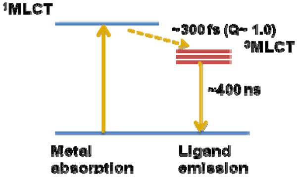
Mechanism of Ru(bpy)₃² emission.⁴³¹

The long fluorescence lifetime of metal complexes can be utilized in oxygen sensing. Ru(bpy)₃²⁺, with a lifetime of several hundred nanoseconds in oxygen-free environment, has been used as an oxygen sensor for monitoring mitochondrial respiration,⁴³³ for cell imaging,^434,435 and to detect cancerous cells⁴³⁶ and tissues.⁴³⁷

Metalloporphyrins

Metalloporphyrins formed by chelating porphyrins with metals such as palladium,⁴³⁸ platinum,⁴³⁹ and gadolinium⁴⁴⁰ (Fig. 42) also belong to a class of luminescent transition metal complexes that have a distinct mechanism of emission. Their red luminescence comes entirely from a triplet state of the aromatic tetrapyrrolic macrocycle populated with the assistance of metals through a “heavy-atom effect”.⁴⁴¹ The phosphorescence lifetime of these molecules varies from microseconds to hundreds of milliseconds.⁴⁴² These materials are highly sensitive to oxygen. Hence, a variety of applications, such as oxygen sensors and hypoxia measurements, has been utilized and reviewed.^442,443 Recently, Gd-porphyrins (Fig. 42) with high quantum phosphorescence yield in NIR and lifetime ∼100 μs have been proposed as potential oxygen sensors for NIR applications.⁴⁴⁰

Lanthanide complexes

Complexes of lanthanides, such as Eu(III), Tb(III), Nd(III), Sm(III), Yb(III), and Dy(III) emit light by a mechanism opposite to the emission of the mentioned transition metal complexes. They utilize ligand-to-metal charge transfer (LMCT) mechanism. The concept of a typical lanthanide based construct is shown in Fig. 44 and a typical lifetime map in Fig. 45. The absorption in the lanthanide complex originates from the capturing of the photon by a chromophoric ligand called an antenna, followed by the intersystem crossing of the excited state into the triplet state and subsequent intramolecular energy transfer from the triplet to the metal. Free lanthanides are not capable of capturing photons due to the forbidden nature of 4f-4f transitions, resulting in extremely low molar absorptivities (ε < 1 M^-1 cm^-1, compared to ε > 10⁵ for a typical organic dye).^444,445 The unique feature of the lanthanide complexes is that 4f electrons are effectively shielded by the filled 5p and 6s orbitals of the metal which protects the emission from the quenchers. For that reason, the luminescence lifetime of the complexes is long (millisecond range for europium and terbium and microsecond range for samarium and dysprosium) and insensitive to oxygen and changes in the environment.

Figure 44.

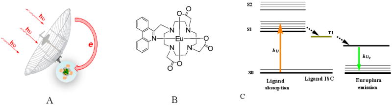
A concept of a lanthanide emissive construct (A), structure of typical lanthanide complex (B)⁵⁴⁵ and the mechanism of emission (C).

Figure 45.

Lifetime map showing silica particles labeled with a Eu(III) complex and suspended in water Reprinted from Ref. 545 Copyright 2000 Elsevier.

A noticeable exception to this stability is a remarkable sensitivity of the lanthanides' lifetime to coordinated water molecules. Excited state energy of the lanthanides is transferred non-radiatively to lower energy lying O-H (and N-H) oscillations, leading to the substantial decrease of the lifetime from 2-3×10³ μs in D₂O to ∼1×10² μs in water for Eu (III) complexes.⁴⁴⁶ The investigation of this effect in sensor design for cell imaging is an active area of research and has been recently reviewed.^301,447,448 The fluorescence lifetime of lanthanides can also be efficiently modulated by the change in the antenna.^445,449 An example of this modulation for oxygen sensing is shown in Fig. 44, where the singlet oxygen causes an oxidation of the aromatic antenna, leading to the alteration of the lifetime of the complex.⁴⁵⁰

A long and stable luminescence lifetime renders lanthanides excellent candidates for time-gated imaging and multiplexing because lanthanides, such as Tb(III), Dy(III), Eu(III), and Sm(III), have mutually distinct emission spectra and different fluorescence lifetimes. A variety of homogeneous and heterogeneous time-gated assays facilitated by the commercial availability of lanthanides complexes suitable for bioconjugation and appropriate instrumentation such as time-gated plate readers have been described^451,452 and reviewed.⁴⁴⁷ Stable lifetimes of the lanthanides have been applied for constructing FRET probes with the lanthanides as donors. Several of these probes (lanthanide-organic dyes⁴⁵³ and lanthanide-fluorescent proteins⁴⁵⁴) have been described.

Microscopy and in vivo imaging with lanthanides is a growing area of research and a number of lanthanide constructs for microscopy and in vivo imaging have been proposed.^455,456 An example of a compound emissive in NIR and potentially suitable for in vivo imaging is shown in Fig. 46. However, the applicability of the lanthanides for biological imaging is limited by the stability of the complexes in aqueous media and their potential toxicity. Also, little is known about the internalization and intracellular localization of metal complexes, although substantial progress in this field has been made and recently reviewed.^301,448 In addition, the long lifetime of lanthanides hampers their utility in biological imaging applications, where fast scanning is required. For example, point-scanning microscopes typically use high excitation power, which causes overpopulation of the long lived excited state, leading to signal decrease and image distortion. Decrease of the beam power restores the image but slows the image acquisition time because longer integration time would be necessary.

Figure 46.

Long lifetime NIR lanthanide Nd(III)- (em. 950 and 1340 nm) based cyclen-ruthenium coordination conjugates and distribution of their lifetimes. Reprinted with permission from ref. Copyright 2006 Reprinted from Ref. 546 Copyright 2006 American Chemical Society.

Upconversion

One of the intriguing and fascinating examples of manipulating with long luminescence lifetimes is a method called upconversion. It refers to the conversion of excitation light to shorter wavelengths or higher energy. The chemistry of the upconverting chelate is similar to the above mentioned lanthanide complexes: a lanthanide ion is complexed with a multidentate chromophoric chelating agent that can be covalently bound to a biomolecule. The simplified mechanism of this process for a water soluble europium complex is shown in Fig. 47.⁴⁵⁷ First, excitation with photons of low energy (λ₁ ∼980 nm) is captured and forms a long lived intermediate state. Non-radiative relaxation is then followed by another excitation with higher energy photons relative to λ₁ (λ₂∼800 nm) to reach the emissive state at λ₃∼550 nm. This two-photon sequential process results in conversion of two photons of low energy to one photon of higher energy with virtually no autofluorescence, providing picomolar sensitivity. Applications of upconversion in biological applications, including imaging, has been recently reviewed.⁴⁵⁸

Figure 47.

Schematics of an upconversion mechanism for Eu(III) complex.⁴⁵⁷

7 Fluorescence lifetime imaging applications

It has long been realized that fluorescence lifetime is a powerful fluorescence parameter in imaging method that could be employed in any situation where fluorescence phenomenon is found. While lifetime spectrophotometers (fluorometers) are commonly used, the concept of lifetime imaging had not realized until the end of the 20^th century due to the lack of fast electronics and computational requirements for data analysis. This impasse changed with the development of time-resolved imaging technique, driven by advances in instrumentation and laser technology. Typical of many paradigm-shifting technological advances, it is not surprising that most of the earlier applications were initiated by groups specializing in physics, engineering, and image reconstructions. Fluorescence lifetime applications in biology and other fields were utilized primarily to validate the quality of the instrument and complement fluorescence intensity measurements. Instrumentation maturity and the availability of commercial instruments have dramatically changed the face of a typical fluorescence lifetime user, uniting physical and biological scientists, engineers, and physicians. Time-resolved studies can now be achieved with a variety of fluorescence techniques, such as single- and two-photon microscopy,^317,459,460 endoscopy,^218,461-465 and tomography.^{317,336,466,467} These efforts have increased the number of reports on the use of fluorescence lifetime in diverse areas of biological imaging. The selected examples below illustrate the tremendous growth and applications of lifetime imaging in recent years.

7.1 Cell biology

The heterogeneous nature of biological samples such as cells and tissues render an environment with a wide range of viscosities. This range spans from low viscosity cytosol and biological liquids to the high viscosity environments seen in cell membranes, DNA, and protein binding sites. Fluorescent rotors with high γ–value probes (see Section 4.1.1) were used in lifetime imaging to measure intracellular viscosity and to distinguish organelles in cells. A meso-substituted Bodipy dye with a rotatable phenyl group (γ = 0.5) was developed for this type of imaging (Fig. 51).^101,468

Figure 51.

FLIM image obtained following 467 nm pulsed excitation of SK-OV-3 cells (A 1.6 ns fluorescence lifetime corresponds to the average intracellular viscosity value of (140±40) cP. Reprinted from Ref. 101 Copyright 2008 American Chemical Society

A variety of fluorescence lifetime sensitive dyes has been applied to study biomembranes. Since the introduction of the fluid mosaic model,⁴⁶⁹ biomembranes have been seen as a complex heterogeneous system composed of microdomains, such as gel, fluid, and liquid phases (known as lipid or membrane rafts) with different mobilities. Gel-phases have rigid, high melting point saturated alkyl chain lipids while the fluid phases are composed of lipids with unsaturated alkyl chains to ensure a greater level of mobility. Rafts are an intermediary phase, enriched in cholesterol, sphingolipids, and saturated lipids. They play an important role in a variety of membrane functions, such as budding, signal transduction, and cell signaling.⁴⁷⁰ The importance of rafts imaging comes from the growing evidence that changes in rafts (composition, location, and clustering) are linked to several pathological conditions such as Alzheimer's disease.⁴⁷¹ Dyes with fluorescence lifetime sensitivity to membrane mobility were employed in imaging of membrane. Rafts differentiation from other microdomains have been recently reviewed.⁴⁷² Thus, the phosphatydilcholine analog C6-NBD-PC, (for NBD structure see Fig. 30),^340,473 the membrane-partitioning dye di-4-ANEPPDHQ,^107,474 and perylene monoimide PMI-COOH,⁴⁷⁵ Rhodamine B with its flexible excited state rotatable alkylamine bonds,³³⁴ Bodipy,⁴⁷⁶ and other lifetime environmental sensitive probes⁴⁷⁷ have been used for these purposes.

Di-4-ANEPPDHQ incorporates into plasma membranes and increases its lifetime in more ordered membranes.¹⁰⁷ The latter feature is often used to differentiate fractions of cell membranes with high level of cholesterol because the increased amount of cholesterol in cell membrane results in higher rigidity. Fig. 48 demonstrates the presence of cholesterol-rich fragments in live HEK293 cells incubated with di-4-ANEPPDHQ dye and the effect of cholesterol removal with β-cyclodextrin from Jurkat cells probed with perylene monoimide (PMI-COOH).⁴⁷⁵

Figure 48.

Structure of molecules and fluorescence lifetime images (a) FLIM map of live HEK293 cells stained with di-4-ANEPPDHQ showing membranes with different orders, Reprinted from Ref. 107 Copyright 2006 Elsevier; (b) obtained for PMI-COOH in: top normal Jurkat cell; bottom: Jurkat cell after cholesterol extraction using methyl- β –cyclodextrin, Reprinted from Ref. 475 Copyright 2007 Elsevier.

The knowledge of interaction between different proteins at every level of cell function is of paramount importance in understanding the molecular mechanism of cell signaling, endocytosis, transport machinery between cells and tissues, regulation of gene expression, and other countless critical processes in a living organism. In conjunction with FRET, fluorescence lifetime has become a useful and rapid method to evaluate protein-protein interactions on a spatial scale less than 10 nm.³⁷³ This approach is superior to diffraction-limited optical resolution. The most critical step of this imaging is labeling of the protein or lipid of interest. This can be achieved by co-expression of the protein with one of the available fluorescent reporters such as fluorescent proteins, or co-localization with organic dyes, or quantum dots. For protein-protein interrogation, labeling with fluorescent proteins is commonly used. The change in the fluorescence lifetime of the FRET donor, attached to a protein or lipid X, is indicative of the close proximity of the protein or lipid Y linked to the FRET acceptor. For example, the self-association of the protein pristine, a highly expressed transmembrane protein in cochlear cells, has been ascertained from the change in fluorescence lifetime of a prestin-CFP in the presence of prestin-YFP.⁴⁷⁸ Recent reviews covering protein-protein studies and their applications based on FRET-FLIM approach,^479-481 including a step-by-step tutorial,⁴⁸² are available. Applications of fluorescence lifetime in lipid-lipid interactions have been recently reviewed.⁴⁷²

7.2 Tissue and small animal lifetime imaging

Imaging of cancer

Ex vivo (cells, tissue) and in vivo (whole body imaging) diagnosis of cancer using lifetimes from endogenous fluorophores and tissues stained with exogenous probes constituent the a significant part of research activities in fluorescence lifetime tissue imaging. Efforts have ranged from unveiling the basic mechanisms of cancer to clinical applications. These include the search for cancer biomarkers in cells, assessing histological architecture of the cancer tissue, early cancer diagnosis, and delineation of the tumor from normal tissue for staging and surgical removal.

Fluorescence lifetime imaging focusing on NAD(P)H autofluorescence has been used extensively to differentiate cancer from noncancerous tissue. Studies found that the decrease in autofluorescence fluorescence lifetime at around 450 nm in fibrosarcoma tumor was associated with a shift of NADH from the bound to the free form.⁴⁸³ Time-resolved fluorescence studies of metastatic and nonmetastatic murine melanoma cell lines, as well as human tumorigenic lung cancer and bronchiolar epithelial cells, showed that the average lifetime of NADH was consistently lower in metastatic cells than in nonmetastatic cells.⁴⁸⁴ A combination of fluorescence lifetime of NADH with fluorescence intensity relative to the emission of tryptophan as an internal standard was applied to differentiate normal from cervical cancer cells.²¹⁷

Fluorescence lifetime imaging of the skin has been used to distinguish basal cell carcinomas (BCCs) from surrounding uninvolved skin for early diagnosis of skin cancer.²²² Disruption of collagen by tumor-associated matrix metalloproteinases from dermal basal cell carcinoma decreases the fluorescence lifetime of collagen, providing a platform for early diagnosis of cancer. Application of this approach to demonstrate its potential in the diagnosis and surgical removal of carcinomas have been reported.²²² Prior to the use of lifetime measurements, earlier efforts to diagnose melanoma using fluorescence intensity techniques faced difficulties due to low signal to noise ratio caused by weak fluorescence intensity, interference from other fluorophores such as NAD(P)H, and high light scattering by the skin.^224,275 In contrast, there are significant differences in the lifetime behavior of melanocytes and keratinocytes. On this basis a clear difference between malignant and normal tissue was observed,⁴⁸⁵ although it was not clear if the change in fluorescence lifetime was due to alteration of melanin structure or NAD(P)H binding.

Two-photon fluorescence lifetime imaging of intracellular NADH in breast cancer cells revealed a heterogeneous environment around the intracellular NADH, which is distinct in breast cancer and normal cells and indicates the sensitivity of fluorescence lifetime in cell pathology.⁴⁸⁶ Fluorescence lifetime imaging of breast tissue biopsies targeting collagen has been proposed to distinguish tissues with collagen dense tumors. These types of tumors have recently been implicated as one of the greatest risk factors for developing breast carcinoma.²¹¹ Time-resolved autofluorescence spectra with subnanosecond temporal resolution of the human bladder, the bronchi, and the esophagus taken during endoscopy revealed lifetime contrasts between normal and neoplastic tissue in all three organs.⁴⁶² However, in contrast to microscopy studies, autofluorescence lifetime conducted in vivo using optical-fiber-based spectrometers in the bronchi of human patients did not show a statistical difference between pre-neoplastic lesions and healthy bronchial mucosa and therefore could not be used for lung cancer diagnosis.⁴⁸⁷

The sensitivity of FAD fluorescence lifetime with respect to protein binding also found its application in the imaging of cancerous tissue. Normal epithelium cells showed lower fluorescence lifetimes, indicating that FAD is primarily in a bound state, while precancerous tissue displayed significantly longer lifetimes, suggesting a substantial amount of released FAD^252,488 (see Fig. 49 as an example). For early tumor diagnosis, time-resolved methods utilizing autofluorescence have shown promise in distinguishing adenomatous from non-adenomatous colon polyps with high sensitivity and specificity. This approach allows for direct endoscopic assessment of colon cancer.⁴⁸⁹

Figure 49.

Fluorescence lifetime images of FAD in vivo, normal (A) low-grade precancer (B) and high-grade precancer (C) squamous epithelium tissues (ex. 890 nm, 400-600 nm emission). The number in the corner indicates depth in μm. Reprinted from Ref. 488 Copyright 2007 National Academy of Sciences, U.S.A.

In breast cancer study with exogeneous dyes, time gated imaging of patient tissues stained with H&E stain revealed diagnostic features specific to malignant tumors. For example, strong signals from elastin rich tissues of stroma and blood vessels are clearly visible (Fig. 50).⁴⁹⁰

Figure 50.

Time-gated intensity images of breast tissue after staining with H&E. (A) Grade 2 invasive ductal carcinoma with desmoplastic stroma. (B) Benign dense collagen and benign epithelium. (C) Vessel (venous). The elastic tissue in the malignancy-associated stroma and the elastic tissue of blood vessels give an extraordinarily bright signal. Reprinted from Ref. 490 Copyright 2003 Wiley-Blackwell.

The relatively long fluorescence lifetime of porphyrins in the spectral range where other endogenous fluorophores are absent can be potentially used for early cancer diagnosis. It is also useful for delineating the boundaries of cancerous tumors for segmental resection and monitoring the effect of therapy. Many researchers have successfully induced porphyrin formation by employing the metabolic machinery of proliferating tumors. In this practice, aminolevulinic acid (5-ALA), a naturally occurring intermediate of heme biosynthesis is typically administered topically. Through a cascade of metabolic reactions, 5-ALA is converted to the highly fluorescent product, protoporphyrin IX, which accumulates in tumor cells to a greater extent compared to normal tissue. The net effect is a resultant increase in the fluorescence lifetime of tumor tissue. Fluorescence lifetime of protoporphyrin IX-induced ALA has been used to differentiate malignant from healthy tissue in brain^491,492 and oral mucosa,⁴⁹³ although differences in the lifetime of protoporphyrin IX in esophagus has not been observed.⁴⁶² Thus, normal brain tissue has an autofluorescence lifetime (upon excitation at 750 nm via two photon mechanism) between 1.5 - 1.8 ns, and the administration of 5-ALA increased the lifetime of tumor tissue to 2.9 ns, allowing clear distinction between the tumor and normal tissue.⁴⁹¹

Intraoperative detection of the residual tumor tissue in cancer surgery remains an important challenge because the extent of tumor removal is related to the prognosis of the disease. Multiphoton excited fluorescence tomography of living tissues provides high-resolution structural and photochemical imaging at a subcellular level and has been applied to glioma tumors. In these studies, fluorescence lifetime imaging demonstrated significantly different decays of the fluorescent signal in tumor versus normal brain, allowing a clear visualization of the tumor-brain interface based on this parameter. Distinct fluorescence lifetimes of endogenous fluorophores were found in different cellular compartments in cultured glioma cells. In combination with fluorescence intensity imaging, these studies demonstrate that normal brain tissue and tumors could be distinguished on the basis of fluorescence lifetime profiles. Therefore, fluorescence lifetime mapping of tissues provides an important tissue analysis strategy that is applicable in intraoperative surgical procedures.^492,494

The development of fluorescence lifetime imaging methods for in vivo use has accelerated their applications for whole-body imaging of cancer in small animals. The seminal work Cubeddu et al.^495-498 used planar illumination and a gated image intensifier to discriminate cancerous and non-cancerous tissue based on autofluorescence and protoporphyrin IX lifetimes. Extension of lifetime imaging using exogenous NIR fluorescent probes was subsequently explored by Reynolds et al.,⁴⁹⁹ where they used frequency domain fluorescence imaging method to extract the lifetimes of the dyes. The wide use of NIR fluorescence lifetime imaging for small animals was delayed for several years until the availability of a commercial time-domain imager (eXplore Optix™) that allowed easy access to the technology. Beginning from 2005, many publications in demonstrating diverse applications of fluorescence lifetime in small animal imaging of diverse diseases have been reported. For example, Bloch et al. demonstrated the feasibility of imaging tumors with receptor-targeted NIR fluorescent probes based on noninvasive fluorescence lifetime imaging.³³⁷ The study further demonstrated significant differences between the lifetime of tumor versus nontumor tissues noninvasively. Fluorescence lifetime imaging provides another dimension for multiplexing information content with multiple fluorophores. In the lifetime regimen, fluorophores with similar excitation and emission spectra can be used, as long as they have resolvable lifetimes and comparable fluorescence quantum yields. Using this approach, Akers et al.³³⁸ recovered the distribution of two NIR fluorescent probes in tumor-bearing rodents by lifetime gating. More recently, the development of diffuse optical tomography-based lifetime techniques has improved the temporal resolution and imaging depth with fluorescent molecular probes.^466,500,501 These developments augur well for the use of fluorescent lifetime imaging of animal models of tumors. Clearly, significant contribution of lifetime studies in tumors will arise from our ability to access the functional status of cancer. This may require the use of fluorescent molecular probes that specifically report the biological event through ratiometric lifetime changes.

Diabetes and kidney pathologies

Diabetes is a worldwide pandemic disease and effective patient monitoring is critical to reduce the devastating effects of the disease. For example, development of methods to report blood glucose levels noninvasively has been the Holy Grail of diabetes-related studies. A recent report demonstrated the feasibility of using fluorescence lifetime of an implanted sensor for continuous measurement of glucose concentration in blood.⁵⁰² Without doubt, noninvasive lifetime-based devices and methods will be developed in future.

Other kidney pathologies are amenable to lifetime-based monitoring technique. The utility of noninvasive fluorescence lifetime imaging in distinguishing between normal and ischemic kidney tissue was demonstrated in a mouse model. The study suggests that fluorescence lifetime analysis of endogenous tissue fluorophores could be used to discriminate ischemic or necrotic tissues by noninvasive in vivo or ex vivo organ imaging.⁵⁰³ NIR lifetime-sensitive probes have been utilized to detect albuminuria, a pathological condition where excess proteins are present in the urine and often an indicator of early stage of diabetes.⁵⁰⁴ An on-line movie showing the change of fluorescence lifetime in a mouse injected with a lifetime sensitive hydrophilic dye is available.⁵⁰⁴

Brain tissue analysis

NADH fluorescence lifetime has been extensively used to assess brain functions⁵⁰⁵ and to differentiate normal from epileptic brain tissue (Fig. 52).⁵⁰⁶ NIR fluorescent probes that exhibit fluorescence lifetime changes when bound to amyloid-beta peptides, the main constituent of amyloid plaques in the brains of Alzheimer's patients, have been synthesized. The probes (see Section 6.1) tested in brain tissue have shown high lifetime sensitivity toward amyloid-beta peptides. Given their blood-brain-barrier permeability, these molecular probes may allow quantitative molecular imaging of amyloid plaques in vivo.²⁹⁶

Figure 52.

FLIM images generated using NADH autofluorescence in the human cortex showing neurons. The bright, punctate spots are NADH-rich mitochondria containing primarily long lifetime bound NADH (blue, 3000 ps - 6000 ps) and unbound NADH (red, ∼300 ps) that are localized in the cytoplasm. Neuropil is composed largely of small-enzyme bound NADH (green, ∼560 ps). Scale bar = 20 μm. Ex/em: 769/<555 nm. Reprinted from Ref. 506 Copyright 2008 Optical Society of America.

Recently synthesized NIAD dyes, such as NIAD-16 (Fig. 30), were designed to form planar geometry upon binding to Aβ fibrils.²⁹⁶ In solution, these dyes show low fluorescence due to unrestricted internal rotation. Upon binding to the amyloid-binding pocket, the rings are rigidly held in a close planar conformation, providing higher fluorescence intensity. Remarkable sensitivity of NIAD dyes to the presence of amyloid plaques has been demonstrated with transgenic mice expressing amyloid precursor protein (APP) (Fig. 53).²⁹⁶

Figure 53.

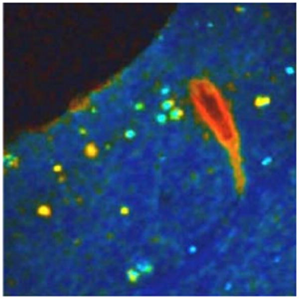
Fluorescence lifetime imaging of APP transgenic mouse brain sections. Vascular amyloid stains at a short lifetime (red), plaques at a medium lifetime (orange to green), and background neuropil at an even longer lifetime (blue). Reprinted from Ref. 296 Copyright 2008 Springer Science+Business Media.

Blood pathologies

The lifetime in a blood vessel has been shown to depend on its composition, displaying characteristic fluorescence lifetimes (Fig. 54).²²⁰ Blood vessels, especially large ones, have strong autofluorescence originating from both collagen and elastin. Differences between the segments rich in elastin could be visualized by determining the characteristic average fluorescence lifetime. The lifetime of blood vessels based on endogenous fluorophores were used to differentiate between healthy and atherosclerotic arterial walls. Gradual increases in the lifetimes from 2.4 ns for normal aorta to 3.9 ns for advanced lesion demonstrated the feasibility of assessing the severity of atherosclerotic lesions by lifetime imaging.^507,508 Further development of the method using a fiber-optic device based on time-resolved laser-induced fluorescence spectroscopy showed the potential of applying the lifetime approach in detecting vulnerable plaques. These unstable plaques are dangerous because they can rupture spontaneously and empty its contents consisting of white blood cells and lipids. This event leads to blood clotting and eventual heart attack or stroke. Fluorescence lifetime imaging has been shown to identify vulnerable plaques with high sensitivity and specificity, thus providing a powerful method to prevent the fatal pathological event.^509,510

Figure 54.

FLIM images of rat aorta lumen showing the lifetime maps, measured with 390 nm (left), 450 nm (middle), and 550 nm (right), using bandpass filters. The arrows indicate an area rich in elastin, ex. 337 nm. Reprinted from Ref. 220 Copyright 2007 IOP Publishing Ltd.

Eye pathologies

Fluorescence lifetime imaging of the human eye is one of the most challenging due to critical imaging limitations that are specific to the eye, such as the maximal permissible exposure to avoid an eye injury induced by light, rapid movement of the eye, and low quantum efficiency of retinal fluorophores which require long exposure time for lifetime measurements. With the advent of more sensitive and rapid electronics, the autofluorescence mapping of the retina for early diagnosis of pathological processes became feasible.²¹⁹

Dental pathologies

Laser-induced time-resolved autofluorescence of human teeth revealed that carious regions exhibited fluorescence decay distinct from healthy, hard dental tissue. The long-lived emitters in the carious lesions were attributed to fluorescent metal-free porphyrin monomers. The fluorescence lifetime can be potentially utilized for early detecction of dental caries.⁵¹¹ The advent of supercontinuous laser sources has further improved the application of this method in dentistry.⁵¹²

Drug delivery and release

Fluorescence lifetime confocal microscopy has been used to study the cellular uptake behavior of the antitumor drug, doxorubicin. This drug is fluorescent and possesses environment-sensitive fluorescence lifetime. The fluorescence lifetime of doxorubicin increases from 1.1 ns in free form to 2.4 ns after binding to DNA, thus providing a method to monitor the release of the drug from a polymeric capsule.⁵¹³ Similarly, the increase of the fluorescence lifetime of the encapsulated NIR dye has also been used to monitor the biodegradability of polymeric nanoparticles used as a model drug carrier in vivo.⁵¹⁴ The nanoparticle shell around a fluorophore forms a tailored microenvironment which defines the initial fluorescence lifetime of the probe. Upon degradation of the shell caused by biological processes (ex. Specific enzymatic activity, change in pH, etc), the fluorophore is exposed to the biological media and alters its lifetime. This approach is illustrated with a biodegradable polymer carrier, whose degradation was monitored using fluorescence lifetime of the dye (Fig. 55). The initial low fluorescence lifetime of the dye surrounded by a hydrophilic poly(ethylene glycol) shell slowly increased upon degradation of the shell from ∼0.35 to ∼0.7 ns.⁵¹⁴

Figure 55.

Fluorescence lifetime maps of NIR fluorescent nanoparticle in vivo at 0-5 days post-injection. Reprinted from Ref. 514 Copyright 2008 American Chemical Society.

Cell trafficking in live animals is a growing area of research that could benefit from the unique features of fluorescence lifetime imaging. For example, dendritic cell therapy is an emerging immunotherapeutic approach for treating advanced cancer as well as for preventing cancer.⁵¹⁵ In this method, the cells, rather than micelles or polymeric nanocapsules, are used as the therapeutic vehicles against the target disease. Fluorescence lifetime imaging of dendritic cells labeled internally with NIR-emissive polymersomes enabled cell tracking in vivo. The method served as a tool to evaluate dendritic-cell-based immunotherapy and provides novel opportunities for in vivo cell tracking by fluorescence imaging.⁵¹⁶

Fluorescence lifetime imaging has been utilized for monitoring drug trafficking and release in human hair. Time-resolved imaging of the intra-tissue diffusion of pharmaceutical and cosmetic components along hair shafts was recently achieved by monitoring the changes in fluorescence lifetime of endogenous keratin and melanin.²⁷³ Similarly, the effect of drugs on the autofluorescence lifetime in skin have been utilized to measure the diffusion and intra-dermal accumulation of topically applied cosmetic and pharmaceutical components in deep skin tissue.^517-519

7.3 Yeast, bacteria and virus detection

Lifetime analysis of yeast strains obtained from lifetime imaging microscopy has been used to differentiate strains on the basis of lifetime distribution within the cells. The cumulative distributions of the lifetime reflecting endogenous flavins for several strains are shown in Fig. 56. The method can be potentially used for quality control in biotechnology.⁵²⁰

Figure 56.

Cumulative distribution function on the average lifetime distributions for different yeast strains A9, Y275, K7 and A13, ex/em. 405/440-540 nm. Reprinted from Ref. 520 Copyright 2008 Wiley-Blackwell.

Timely and effective detection of bacterial and viral infections is critical for preventing the spread and provide effective clinical management of microbial deases. Thus, fluorescence lifetime of intrinsic fluorophores, such as tryptophans, has been used to differentiate gram-positive from gram-negative bacteria.⁵²¹ Time-resolved approaches using intrinsic fluorescence lifetime was used to detect bacteria on meat surfaces⁵²² and to differentiate active from inactive forms of bacteria, bacteria colonies, and biofilms.⁵²³ In the latter work, the authors utilized exogenous dye SYTO 13, which has lifetime sensitivity to RNA/DNA ratio. Shorter lifetimes correspond to DNA–rich slow growing bacteria.

Feces and other excrements from sick animals and humans can spread many diseases if they accidentally are exposed to food and water. Fluorescence lifetime imaging has been proposed to identify these problems. For example, the fluorescence lifetime image of an apple contaminated with feces provided excellent visualization with high contrast between the apples and feces-treated spots (Fig. 57).²¹⁴

Figure 57.

Fluorescence lifetime images of an apple artificially contaminated with the three feces spots (Ex/em 418/670 nm). Reprinted from Ref. 214 Copyright 2008 Optical Society of America.

For virus detections, an interesting approach utilizing a combination of fluorescence lifetime and specifically designed cell lines have been described.⁵²⁴ The method uses a virus-specific HeLa-based cell line encoded with FRET assemblies. Upon a viral infection, the encoded viral genome protease releases into the cytoplasm of the host cell and cleaves the protease-sensitive FRET construct composed of fluorescent proteins GFP2 and DsRed2, linked by a cleavage protease recognition site. The cleavage results in an increase of the fluorescence lifetime and indicates the presence of the target virus.⁵²⁴

7.4 Materials sciences and forensic applications

In addition to fluorescence lifetime imaging in biology and medicine, time-resolved imaging is quickly infiltrating other fields such as the arts, sciences, engineering, and forensics.

Microfluidic devices

Fluorescence lifetime imaging has been used in microfluidic devices to monitor and adjust a variety of parameters such as temperature^525,526 and mixing characteristics.¹⁸⁵ N-ethylenic group in Rhodamine B (Fig. 58) is free to rotate and at higher temperatures the increased rotation decreases its fluorescence lifetime. In contrast, the lifetime of Rhodamine 101, with a fixed N-ethyl bond, is practically insensitive to temperature.⁵²⁷ This principle has been utilized to characterize temperature in a micrufluidic dual beam laser trap⁵²⁵ and as a temperature sensor for continuous adjustment of temperature in a microfluidic polymer chain reaction device.^526,528 The example of temperature sensing based on fluorescence lifetime of Rhodamine B is shown in Fig. 58.

Forensics

One of the challenges in criminal investigation is the lack of detection techniques for imaging latent fingerprints. Many existing techniques based on fluorescence intensity measurements fail in the presence of a strong fluorescence background. To overcome this problem, staining the fingermarks with a fluorescent dye with longer fluorescence lifetime, such as fluorescent lanthanides complexes reacting with amino acids from the fingerprints in situ, have been utilized.^529,530 Additionally, lifetime-based imaging of fingerprints using a variety of organic dyes, including the currently used fluorescence powder Blitz-green™ (proprietary structure) with a fluorescence lifetime of 8.96 ns, has been utilized to eliminate fluorescence background and to detect latent fingermarks with higher contrast (Fig. 59).^531,532

Figure 59.

The intensity image (a) and fluorescence lifetime image (b) of the blitz-green-treated finger mark samples on postcard substrate. Reprinted from Ref. 532 Copyright 2006 Elsevier.

Other examples include artwork analysis,^533,534 visualization of mechanical defects with fluorescent pressure-sensitive and temperature-sensitive paints⁵³⁵ and specially designed polymers,⁵³⁶ measurement of the distribution of hot gases in aeronautics,^537,538 and the design of counterfeit materials.⁵³⁹

8 Conclusions and future directions

Techniques for fluorescence lifetime measurements have undergone incredible transformations since Edward Becquerel invented a device to measure luminescence lifetime of uranium salts in 1859. The subsequent development of fluorometers facilitated the formulation of excellent theoretical basis for fluorescence lifetime of diverse compounds and materials. Recent advances in laser technology, computational power, and imaging algorithms have extended the application of fluorescence lifetime method into medical imaging. Initial applications of fluorescence lifetime in cell studies focused on autofluorescence lifetimes of endogenous fluorophores. The lifetime signatures of these biomolecules can be altered by changes in normal cell physiology or pathologic conditions. Through ratiometric analysis of different endogenous fluorophore lifetimes, it is possible to quantify relevant molecular processes at the cellular level. The use of autofluorescence lifetimes in biological imaging also provides a direct path to human translation of the cell-based studies. For these reasons, diverse group of researchers have been able to characterize and identify lesions in humans by fluorescence lifetime techniques. In parallel to autofluorescence lifetimes, scientists have accelerated the development of new fluorophores and luminescent materials for lifetime studies. In most biological studies, the unique ability to perturb the fluorescence lifetime in response to specific biological event or background subtraction by using fluorophores with distinct lifetimes has improved image analysis and enriched the content of the intended diagnostic information. Depending on the ultimate goal of the study, molecular probes with fixed or variable lifetimes can be used. The availability of a commercial small animal imaging system has extended the application of fluorescence lifetime studies in small animal beyond the confines of instrumentation experts. Today, numerous preclinical studies in animal models of human diseases have increased dramatically. The emergence of newer diffuse optical tomography (DOT)-based lifetime devices will further enhance the quantitative accuracy and imaging depth by this technique. Biological applications of fluorescence lifetime imaging are only in the nascent stage. With its ability to provide unique and complementary diagnostic information, we envisage a seamless integration of fluorescence lifetime method into the family of molecular imaging tools. As with all optical imaging methods, fluorescence lifetime technology has its own challenges. Reliable methods to deconvolve the complex decay profile of multiple lifetimes and quantitatively report lifetime changes in heterogeneous tissue are need. Nonetheless, this technology platform will certainly play important roles in monitoring treatment response, identifying tumor margins, and delineating normal from disease tissues. The availability of commercial fiber-based DOT-based lifetime devices in future will expand the application of this method to endoscope-accessible tissues and organs.

Figure 8.

Frequency domain data obtained from conversion of time domain data shown in Figure 7 via Fourier transform. Left: Phase and modulation at 80 MHz frequency, excitation (black), emission (red – ICG, blue- PPC-BF2) illustrating the phase-angle shift (φ) and demodulation ratio (M). Right: fluorescence lifetime data simulated at different frequencies different frequencies (courtesy of R. Nothdurft and J. Culver, Washington University, St. Louis).

References

- 1.McGown LB, Nithipatikom K. Appl Spectrosc Rev. 2000;35:353. [Google Scholar]
- 2.Chen Y, Periasamy A. Microsc Res Tech. 2004;63:72. doi: 10.1002/jemt.10430. [DOI] [PubMed] [Google Scholar]
- 3.Lakowicz JR. Principles of fluorescence spectroscopy. 3rd. Springer; New York: 2006. [Google Scholar]
- 4.Becker W, Bergmann A, Biskup C. Microsc Res Tech. 2007;70:403. doi: 10.1002/jemt.20432. [DOI] [PubMed] [Google Scholar]
- 5.Becker W, Bergmann A. In: Handbook of Biomedical Nonlinear Optical Microscopy. Master BR, So P, editors. Oxford University Press, USA; New York, NY: 2008. [Google Scholar]
- 6.Patting M. In: Standardization and Quality Assurance in Fluorescence Measurements I. Resch-Genger U, editor. Vol. 5 Springer-Verlag; Berlin, Heidelberg: 2008. [Google Scholar]
- 7.Boens N, Ameloot M, Valeur B. In: Standardization and Quality Assurance in Fluorescence Measurements I. Resch-Genger U, editor. Vol. 5 Springer-Verlag; Berlin, Heidelberg: 2008. [Google Scholar]
- 8.Becker W. Advanced time-correlated single photon counting techniques. Springer; Berlin; New York: 2005. [Google Scholar]
- 9.Becker W. The bh TCSPC Handbook. Third. Becker & Hickl Gmbh; 2008. [Google Scholar]
- 10.Periasamy A, Clegg RM, editors. FLIM Microscopy in Biology and Medicine. Chapman & Hall/CRC; 2009. [Google Scholar]
- 11.Crew H, Fraunhofer Jv, Brace DB. The Wave theory, light and spectra. Arno Press: New York; 1981. [Google Scholar]
- 12.Stokes GG. Phil Trans R Soc Lond. 1852;142:463. [Google Scholar]
- 13.Emsmann H. Ann Phys. 1862;190:651. [Google Scholar]
- 14.Fizeau H. CR Acad Sci. 1849;1849:90. [Google Scholar]
- 15.Becquerel E. Ann Chimie Physique. 1859;3:5. [Google Scholar]
- 16.Nichols EL, Howes HL, Merritt EG, Wilber DT, Wick FG. Fluorescence of the uranyl salts. Carnegie Institution of Washington; Washington: 1919. [Google Scholar]
- 17.O'Haver TC, Winefordner JD. Anal Chem. 1966;38:602. [Google Scholar]
- 18.Kerr J. Philos Mag. 1875;50:337. [Google Scholar]
- 19.Abraham H, Lemoine J. Séances Soc Franç Physique. 1899;44:155. [Google Scholar]
- 20.Beams JW. Rev Sci Instrum. 1930;1:780. [Google Scholar]
- 21.Tumerman LA. Usp Fiz Nauk. 1947;33:218. [Google Scholar]
- 22.Wood RW. Proc R Soc London, Ser A. 1921;99:362. [Google Scholar]
- 23.Rawcliffe RD. Rev Sci Instrum. 1942;13:413. [Google Scholar]
- 24.Yu W, Pellegrino F, Grant M, Alfano RR. J Chem Phys. 1977;67:1766. [Google Scholar]
- 25.Gundlach L, Piotrowiak P. Opt Lett. 2008;33:992. doi: 10.1364/ol.33.000992. [DOI] [PubMed] [Google Scholar]
- 26.Gottling PF. Phys Rev. 1923;22:566. [Google Scholar]
- 27.Beams JW. J Opt Soc Am. 1926;13:597. [Google Scholar]
- 28.Gaviola E. Ann Phys. 1926;81:681. [Google Scholar]
- 29.Beams JW. Phys Rev. 1926;28:475. [Google Scholar]
- 30.Gaviola E. Phys Rev. 1929;33:1023. [Google Scholar]
- 31.de Melo JS, Takato S, Sousa M, Melo MJ, Parola AJ. Chem Commun. 2007:2624. doi: 10.1039/b618926a. [DOI] [PubMed] [Google Scholar]
- 32.Wiliams CHG. Trans Roy Soc Edinburgh. 1856;21:377. [Google Scholar]
- 33.Wagner JRv. A handbook of chemical technology. J.& A. Churchill; London: 1872. [Google Scholar]
- 34.Baeyer A. Ber d Chem Ges. 1871;4:555. [Google Scholar]
- 35.Am J Dent Sci. 1878;12:425. [Google Scholar]
- 36.Baeyer A. Ber d Chem Ges. 1875;8:146. [Google Scholar]
- 37.Willm E, Bouchardat G, Girard C. Chem Industrie. 1878;11:370. [Google Scholar]
- 38.Le Royer A. Ann Chem. 1887;238:350. [Google Scholar]
- 39.Society of dyers and colourists. Rowe FM. Colour index. 1st. The Society; Bradford Yorkshire: 1924. [Google Scholar]
- 40.Borissow P. Journ Russ Phys-Chem Ges. 1906;37:249. [Google Scholar]
- 41.Weigert F. Verhand d deut phys geselsch. 1920;23:100. [Google Scholar]
- 42.Vavilov SI, Levshin VL. Z Phys. 1923;16:135. [Google Scholar]
- 43.Levshin VL. Z Phys. 1925;32:307. [Google Scholar]
- 44.Vavilov SI. Z Phys. 1924;22:266. [Google Scholar]
- 45.Crosby GA, Demas JN. J Phys Chem. 1971;75:991. [Google Scholar]
- 46.Perrin F. J Phys Radium. 1926;7:390. [Google Scholar]
- 47.Gaviola E. Z Phys. 1926;35:748. [Google Scholar]
- 48.Ross JA, Jameson DM. Photochem Photobiol Sci. 2008;7:1301. doi: 10.1039/b804450n. [DOI] [PubMed] [Google Scholar]
- 49.Valeur B. Molecular fluorescence: principles and applications. Wiley-VCH; Weinheim; New York: 2002. [Google Scholar]
- 50.Valeur B, Brochon JC. New trends in fluorescence spectroscopy : applications to chemical and life science. Springer; New York: 2001. [Google Scholar]
- 51.Berezin MY, Lee H, Akers W, Achilefu S. Biophys J. 2007;93:2892. doi: 10.1529/biophysj.107.111609. [DOI] [PMC free article] [PubMed] [Google Scholar]
- 52.Berezin MY, Akers WJ, Guo K, Fischer GM, Daltrozzo E, Zumbusch A, Achilefu S. Biophys J. 2009;97:L22. doi: 10.1016/j.bpj.2009.08.022. [DOI] [PMC free article] [PubMed] [Google Scholar]
- 53.Perrin F. Ann Phys. 1929;12:169. [Google Scholar]
- 54.Hammer M, Schweitzer D, Richter S, Konigsdorffer E. Physiol Meas. 2005;26:N9. doi: 10.1088/0967-3334/26/4/N01. [DOI] [PubMed] [Google Scholar]
- 55.Spencer RD, Weber G. J Chem Phys. 1970;52:1654. [Google Scholar]
- 56.Fisz JJ. J Phys Chem A. 2007;111:12867. doi: 10.1021/jp0775855. [DOI] [PubMed] [Google Scholar]
- 57.König K, Uchugonova A. In: FLIM Microscopy in Biology and Medicine. Periasamy A, Clegg R, editors. Chapman & Hall; 2009. [Google Scholar]
- 58.Göppert-Mayer M. Ann Phys. 1931;401:273. [Google Scholar]
- 59.Kaiser W, Garrett CGB. Phys Rev Lett. 1961;7:229. [Google Scholar]
- 60.Denk W, Strickler JH, Webb WW. Science. 1990;248:73. doi: 10.1126/science.2321027. [DOI] [PubMed] [Google Scholar]
- 61.König K, So PTC, Mantulin WW, Tromberg BJ, Gratton E. J Microsc. 1996;183:197. [PubMed] [Google Scholar]
- 62.Peter M, Ameer-Beg SM, Hughes MK, Keppler MD, Prag S, Marsh M, Vojnovic B, Ng T. Biophys J. 2005;88:1224. doi: 10.1529/biophysj.104.050153. [DOI] [PMC free article] [PubMed] [Google Scholar]
- 63.Krishnan RV, Masuda A, Centonze VE, Herman B. J Biomed Opt. 2003;8:362. doi: 10.1117/1.1577574. [DOI] [PubMed] [Google Scholar]
- 64.Becker W, Bergmann A, Hink MA, König K, Benndorf K, Biskup C. Microsc Res Tech. 2004;63:58. doi: 10.1002/jemt.10421. [DOI] [PubMed] [Google Scholar]
- 65.Fine S, Hansen W. Appl Opt. 1971;10:2350. doi: 10.1364/AO.10.002350. [DOI] [PubMed] [Google Scholar]
- 66.Campagnola PJ, Loew LM. Nat Biotechnol. 2003;21:1356. doi: 10.1038/nbt894. [DOI] [PubMed] [Google Scholar]
- 67.Salafsky JS, Cohen B. J Phys Chem B. 2008;112:15103. doi: 10.1021/jp803703m. [DOI] [PubMed] [Google Scholar]
- 68.Schenke-Layland K. J Biophotonics. 2008;1:451. doi: 10.1002/jbio.200810045. [DOI] [PMC free article] [PubMed] [Google Scholar]
- 69.Einstein A. Phys Z. 1917;18:121. [Google Scholar]
- 70.Tolman RC. Phys Rev. 1924;23:693. [Google Scholar]
- 71.Lewis GN, Kasha M. J Am Chem Soc. 1945;67:994. [Google Scholar]
- 72.Strickler SJ, Berg RA. J Chem Phys. 1962;37:814. [Google Scholar]
- 73.Lee H, Berezin MY, Henary M, Strekowski L, Achilefu S. J Photochem Photobiol, A. 2008;200:438. doi: 10.1016/j.jphotochem.2008.09.008. [DOI] [PMC free article] [PubMed] [Google Scholar]
- 74.El-Bayoumi MA, Dalle JP, O'Dwyer F. J Am Chem Soc. 1970;92:3494. [Google Scholar]
- 75.Frank HA, Desamero RZB, Chynwat V, Gebhard R, van der Hoef I, Jansen FJ, Lugtenburg J, Gosztola D, Wasielewski MR. J Phys Chem, A. 1997;101:149. [Google Scholar]
- 76.Susdorf T, Bansal AK, Penzkofer A, Guo SL, Shi JM. Chem Phys. 2007;333:49. [Google Scholar]
- 77.van Manen HJ, Verkuijlen P, Wittendorp P, Subramaniam V, van den Berg TK, Roos D, Otto C. Biophys J. 2008;94:L67. doi: 10.1529/biophysj.107.127837. [DOI] [PMC free article] [PubMed] [Google Scholar]
- 78.Suhling K, Siegel J, Phillips D, French PM, Leveque-Fort S, Webb SE, Davis DM. Biophys J. 2002;83:3589. doi: 10.1016/S0006-3495(02)75359-9. [DOI] [PMC free article] [PubMed] [Google Scholar]
- 79.Levshin VL. Z Phys. 1931;72:382. [Google Scholar]
- 80.Levshin VL. Usp Fiz Nauk. 1958;64:55. [Google Scholar]
- 81.Merer AJ, Mulliken RS. Chem Rev. 1969;69:639. [Google Scholar]
- 82.Sumitani M, Yoshihara K. Bull Chem Soc Jpn. 1982;55:85. [Google Scholar]
- 83.Doukas AG, Junnarkar MR, Alfano RR, Callender RH, Kakitani T, Honig B. Proc Nat Acad Sci USA. 1984;81:4790. doi: 10.1073/pnas.81.15.4790. [DOI] [PMC free article] [PubMed] [Google Scholar]
- 84.Logunov SL, Masciangioli TM, Kamalov VF, El-Sayed MA. J Phys Chem, B. 1998;102:2303. [Google Scholar]
- 85.Andersson PO, Gillbro T. J Chem Phys. 1995;103:2509. [Google Scholar]
- 86.Wiedemann E, Schmidt GC. Ann Phys. 1896;58:103. [Google Scholar]
- 87.Becquerel H, Becquerel J, Onnes HK. Proc KNAW Phys lab Leiden. 1910;12:76. [Google Scholar]
- 88.Lenard P, Onnes HK, Pauli WE. Proc KNAW, Phys lab Leiden. 1910;12:157. [Google Scholar]
- 89.Stark J, Meyer R. Physik Z. 1907;8:250. [Google Scholar]
- 90.Jue T. Fundamental concepts in biophysics. Humana; New York: 2009. [Google Scholar]
- 91.Lakowicz JR, Prendergast FC. Biophys J. 1978;24:213. doi: 10.1016/S0006-3495(78)85357-0. [DOI] [PMC free article] [PubMed] [Google Scholar]
- 92.Imasaka T, Moore DS, Vo-Dinh T. Pure Appl Chem. 2003;75:975. [Google Scholar]
- 93.Zhang F, Votava O, Lacey AR, Kable SH. J Phys Chem, A. 2001;105:5111. [Google Scholar]
- 94.Bartl K, Funk A, Gerhards M. J Chem Phys. 2008;129:234306. doi: 10.1063/1.3037023. [DOI] [PubMed] [Google Scholar]
- 95.Itoh M. Pure Appl Chem. 1993;65:1629. [Google Scholar]
- 96.Förster T, Hoffmann G. Z Phys Chem. 1971;75:63. [Google Scholar]
- 97.Kaschke M, Kleinschmidt J, Wilhelmi B. Laser Chem. 1985;5:119. [Google Scholar]
- 98.Demchenko AP, Mély Y, Duportail G, Klymchenko AS. Biophys J. 2009;96:3461. doi: 10.1016/j.bpj.2009.02.012. [DOI] [PMC free article] [PubMed] [Google Scholar]
- 99.Haidekker MA, Ling TT, Anglo M, Stevens HY, Frangos JA, Theodorakis EA. Chem Biol. 2001;8:123. doi: 10.1016/s1074-5521(00)90061-9. [DOI] [PubMed] [Google Scholar]
- 100.Haidekker MA, Theodorakis EA. Org Biomol Chem. 2007;5:1669. doi: 10.1039/b618415d. [DOI] [PubMed] [Google Scholar]
- 101.Kuimova MK, Yahioglu G, Levitt JA, Suhling K. J Am Chem Soc. 2008;130:6672. doi: 10.1021/ja800570d. [DOI] [PubMed] [Google Scholar]
- 102.Berezin MY, Lee H, Akers W, Nikiforovich G, Achilefu S. Molecular Probes for Biomedical Applications II. Proc. SPIE; San Jose. 2008; p. 68670J. [Google Scholar]
- 103.Haidekker MA, Brady TP, Lichlyter D, Theodorakis EA. Bioorg Chem. 2005;33:415. doi: 10.1016/j.bioorg.2005.07.005. [DOI] [PubMed] [Google Scholar]
- 104.Singh AK, Das J. Biophys Chem. 1998;73:155. doi: 10.1016/s0301-4622(98)00158-6. [DOI] [PubMed] [Google Scholar]
- 105.Benninger R, Hofmann O, Önfelt B, Munro I, Chris Davis D, Neil M, French P, de Mello A. Angew Chem Int Ed. 2007;46:2228. doi: 10.1002/anie.200604112. [DOI] [PubMed] [Google Scholar]
- 106.Schneckenburger H, Stock K, Lyttek M, Strauss WS, Sailer R. Photochem Photobiol Sci. 2004;3:127. doi: 10.1039/b306129a. [DOI] [PubMed] [Google Scholar]
- 107.Owen DM, Lanigan PMP, Dunsby C, Munro I, Grant D, Neil MAA, French PMW, Magee AI. Biophys J. 2006;90:L80. doi: 10.1529/biophysj.106.084673. [DOI] [PMC free article] [PubMed] [Google Scholar]
- 108.Togashi DM, Ryder AG. J Fluoresc. 2006;16:153. doi: 10.1007/s10895-005-0029-9. [DOI] [PubMed] [Google Scholar]
- 109.Terpetschnig E, Szmacinski H, Ozinskas A, Lakowicz JR. Anal Biochem. 1994;217:197. doi: 10.1006/abio.1994.1109. [DOI] [PubMed] [Google Scholar]
- 110.Jisha VS, Arun KT, Hariharan M, Ramaiah D. J Am Chem Soc. 2006;128:6024. doi: 10.1021/ja061301x. [DOI] [PubMed] [Google Scholar]
- 111.Abugo OO, Nair R, Lakowicz JR. Anal Biochem. 2000;279:142. doi: 10.1006/abio.2000.4486. [DOI] [PMC free article] [PubMed] [Google Scholar]
- 112.Berezin MY, Lee H, Akers W, Nikiforovich G, Achilefu S. Photochem Photobiol. 2007;83:1371. doi: 10.1111/j.1751-1097.2007.00173.x. [DOI] [PubMed] [Google Scholar]
- 113.Pavlovich VS. Biopolymers. 2006;82:435. doi: 10.1002/bip.20464. [DOI] [PubMed] [Google Scholar]
- 114.Bertolino CA, Ferrari AM, Barolo C, Viscardi G, Caputo G, Coluccia S. Chem Phys. 2006;330:52. doi: 10.1007/s10895-006-0094-8. [DOI] [PubMed] [Google Scholar]
- 115.Cramer CJ, Famini GR, Lowrey AH. Acc Chem Res. 1993;26:599. [Google Scholar]
- 116.Lippert E. Z Elektrochem Angew Phys Chem. 1957;61:962. [Google Scholar]
- 117.Mataga N, Kaifu Y, Koizumi M. Bull Chem Soc Japan. 1956;29:465. [Google Scholar]
- 118.Hsieh CC, Cheng YM, Hsu CJ, Chen KY, Chou PT. J Phys Chem, A. 2008;112:8323. doi: 10.1021/jp804216u. [DOI] [PubMed] [Google Scholar]
- 119.Knyukshto V, Zenkevich E, Sagun E, Shulga A, Bachilo S. Chem Phys Lett. 1999;304:155. [Google Scholar]
- 120.McHedlov-Petrossyan NO, Vodolazkaya NA, Surov YN, Samoylov DV. Spectrochim Acta, A. 2005;61:2747. doi: 10.1016/j.saa.2004.09.030. [DOI] [PubMed] [Google Scholar]
- 121.Syage JA, Steadman J. J Chem Phys. 1991;95:2497. [Google Scholar]
- 122.Chattoraj M, King BA, Bublitz GU, Boxer SG. Proc Natl Acad Sci U S A. 1996;93:8362. doi: 10.1073/pnas.93.16.8362. [DOI] [PMC free article] [PubMed] [Google Scholar]
- 123.Bhattacharyya K. Acc Chem Res. 2002;36:95. doi: 10.1021/ar020067m. [DOI] [PubMed] [Google Scholar]
- 124.Hansen JE, Pines E, Fleming GR. J Phys Chem. 2002;96:6904. [Google Scholar]
- 125.Sukul D, Pal SK, Mandal D, Sen S, Bhattacharyya K. J Phys Chem, B. 2000;104:6128. [Google Scholar]
- 126.Cohen B, Huppert D, Solntsev KM, Tsfadia Y, Nachliel E, Gutman M. J Am Chem Soc. 2002;124:7539. doi: 10.1021/ja012646c. [DOI] [PubMed] [Google Scholar]
- 127.Berezin MY, Kao J, Achilefu S. Chem Eur J. 2009;15:3560. doi: 10.1002/chem.200801784. [DOI] [PMC free article] [PubMed] [Google Scholar]
- 128.Dance ZEX, Mickley SM, Wilson TM, Ricks AB, Scott AM, Ratner MA, Wasielewski MR. J Phys Chem, A. 2008;112:4194. doi: 10.1021/jp800561g. [DOI] [PubMed] [Google Scholar]
- 129.Menzel R, Thiel E. Chem Phys Lett. 1998;291:237. [Google Scholar]
- 130.Boens N, Qin W, Basaric N, Hofkens J, Ameloot M, Pouget J, Lefevre JP, Valeur B, Gratton E, vandeVen M, Silva ND, Engelborghs Y, Willaert K, Sillen A, Rumbles G, Phillips D, Visser AJWG, van Hoek A, Lakowicz JR, Malak H, Gryczynski I, Szabo AG, Krajcarski DT, Tamai N, Miura A. Anal Chem. 2007;79:2137. doi: 10.1021/ac062160k. [DOI] [PMC free article] [PubMed] [Google Scholar]
- 131.Khajehpour M, Troxler T, Vanderkool JM. Photochem Photobiol. 2004;80:359. doi: 10.1562/2004-04-01-RA-131. [DOI] [PubMed] [Google Scholar]
- 132.Larkin JM, Donaldson WR, Foster TH, Knox RS. Chem Phys. 1999;244:319. [Google Scholar]
- 133.Förster T. Ann Phys. 1948;437:55. [Google Scholar]
- 134.Medintz IL, Clapp AR, Mattoussi H, Goldman ER, Fisher B, Mauro JM. Nat Mater. 2003;2:630. doi: 10.1038/nmat961. [DOI] [PubMed] [Google Scholar]
- 135.Clapp A, Medintz I, Mattoussi H. Chemphyschem. 2006;7:47. doi: 10.1002/cphc.200500217. [DOI] [PubMed] [Google Scholar]
- 136.Qian H, Georgi C, Anderson N, Green AA, Hersam MC, Novotny L, Hartschuh A. Nano Lett. 2008;8:1363. doi: 10.1021/nl080048r. [DOI] [PubMed] [Google Scholar]
- 137.Hering VR, Gibson G, Schumacher RI, Faljoni-Alario A, Politi MJ. Bioconjugate Chem. 2007;18:1705. doi: 10.1021/bc700147j. [DOI] [PubMed] [Google Scholar]
- 138.Tramier M, Coppey-Moisan M. Methods Cell Biol. 2008;85:395. doi: 10.1016/S0091-679X(08)85017-0. [DOI] [PubMed] [Google Scholar]
- 139.Piston DW, Rizzo MA. Methods Cell Biol. 2008;85:415. doi: 10.1016/S0091-679X(08)85018-2. [DOI] [PubMed] [Google Scholar]
- 140.Gryczynski Z, Gryczynski I, Lakowicz JR. In: Molecular Imaging. 1. Periasamy A, Day R, editors. Oxford University Press; New York, NY: 2005. [Google Scholar]
- 141.Gadella TW, editor. FRET and FLIM Techniques. 1. Vol. 33 Elsevier Science; 2008. [Google Scholar]
- 142.Zhang Z, Fan J, Cheney PP, Berezin MY, Edwards WB, Akers WJ, Shen D, Liang K, Culver JP, Achilefu S. Mol Pharmaceutics. 2009;6:416. doi: 10.1021/mp800264k. [DOI] [PMC free article] [PubMed] [Google Scholar]
- 143.Kenworthy AK. Methods. 2001;24:289. doi: 10.1006/meth.2001.1189. [DOI] [PubMed] [Google Scholar]
- 144.Albertazzi L, Arosio D, Marchetti L, Ricci F, Beltram F. Photochem Photobiol. 2009;85:287. doi: 10.1111/j.1751-1097.2008.00435.x. [DOI] [PubMed] [Google Scholar]
- 145.Clegg R. Biophotonics Int. 2004;11:42. [Google Scholar]
- 146.Dale RE, Eisinger J, Blumberg WE. Biophys J. 1979;26:161. doi: 10.1016/S0006-3495(79)85243-1. [DOI] [PMC free article] [PubMed] [Google Scholar]
- 147.Roy R, Hohng S, Ha T. Nat Methods. 2008;5:507. doi: 10.1038/nmeth.1208. [DOI] [PMC free article] [PubMed] [Google Scholar]
- 148.Clegg RM. Methods Enzymol. 1992;211:353. doi: 10.1016/0076-6879(92)11020-j. [DOI] [PubMed] [Google Scholar]
- 149.Murphy MC, Rasnik I, Cheng W, Lohman TM, Ha TJ. Biophys J. 2004;86:2530. doi: 10.1016/S0006-3495(04)74308-8. [DOI] [PMC free article] [PubMed] [Google Scholar]
- 150.Lee NK, Kapanidis AN, Wang Y, Michalet X, Mukhopadhyay J, Ebright RH, Weiss S. Biophys J. 2005;88:2939. doi: 10.1529/biophysj.104.054114. [DOI] [PMC free article] [PubMed] [Google Scholar]
- 151.van der Meer BW. J Biotechnol. 2002;82:181. doi: 10.1016/s1389-0352(01)00037-x. [DOI] [PubMed] [Google Scholar]
- 152.Lankiewicz L, Malicka J, Wiczk W. Acta Biochim Pol. 1997;44:477. [PubMed] [Google Scholar]
- 153.Yasuda R, Masaike T, Adachi K, Noji H, Itoh H, Kinosita K. Proc Natl Acad Sci USA. 2003;100:9314. doi: 10.1073/pnas.1637860100. [DOI] [PMC free article] [PubMed] [Google Scholar]
- 154.Cherny D, Eperon I, Bagshaw C. Eur Biophys J. 2009;38:395. doi: 10.1007/s00249-008-0383-z. [DOI] [PubMed] [Google Scholar]
- 155.Corry B, Jayatilaka D, Martinac B, Rigby P. Biophys J. 2006;91:1032. doi: 10.1529/biophysj.106.080713. [DOI] [PMC free article] [PubMed] [Google Scholar]
- 156.Berney C, Danuser G. Biophys J. 2003;84:3992. doi: 10.1016/S0006-3495(03)75126-1. [DOI] [PMC free article] [PubMed] [Google Scholar]
- 157.VanBeek DB, Zwier MC, Shorb JM, Krueger BP. Biophys J. 2007;92:4168. doi: 10.1529/biophysj.106.092650. [DOI] [PMC free article] [PubMed] [Google Scholar]
- 158.Pham E, Chiang J, Li I, Shum W, Truong K. Structure. 2007;15:515. doi: 10.1016/j.str.2007.03.009. [DOI] [PubMed] [Google Scholar]
- 159.Corry B, Jayatilaka D. Biophys J. 2008;95:2711. doi: 10.1529/biophysj.107.126243. [DOI] [PMC free article] [PubMed] [Google Scholar]
- 160.Harriman A, Izzet G, Ziessel R. J Am Chem Soc. 2006;128:10868. doi: 10.1021/ja0631448. [DOI] [PubMed] [Google Scholar]
- 161.Dexter DL. J Chem Phys. 1953;21:836. [Google Scholar]
- 162.Hassoon S, Lustig H, Rubin MB, Speiser S. J Phys Chem. 1984;88:6367. [Google Scholar]
- 163.Speiser S, Hassoon S, Rubin MB. J Phys Chem. 1986;90:5085. [Google Scholar]
- 164.Speiser S. Chem Rev. 1996;96:1953. doi: 10.1021/cr941193+. [DOI] [PubMed] [Google Scholar]
- 165.Murphy CB, Zhang Y, Troxler T, Ferry V, Martin JJ, Jones WE. J Phys Chem, B. 2004;108:1537. [Google Scholar]
- 166.Mondal JA, Ramakrishna G, Singh AK, Ghosh HN, Mariappan M, Maiya BG, Mukherjee T, Palit DK. J Phys Chem, A. 2004;108:7843. [Google Scholar]
- 167.Pispisa B, Palleschi A, Mazzuca C, Stella L, Valeri A, Venanzi M, Formaggio F, Toniolo C, Broxterman QB. J Fluoresc. 2002;12:213. doi: 10.1002/bip.10118. [DOI] [PubMed] [Google Scholar]
- 168.Soler M, McCusker JK. J Am Chem Soc. 2008;130:4708. doi: 10.1021/ja077096i. [DOI] [PubMed] [Google Scholar]
- 169.Hurley DJ, Tor Y. J Am Chem Soc. 2002;124:13231. doi: 10.1021/ja020172r. [DOI] [PubMed] [Google Scholar]
- 170.Hsu CP. Acc Chem Res. 2009;42:509. doi: 10.1021/ar800153f. [DOI] [PubMed] [Google Scholar]
- 171.Levy ST, Rubin MB, Speiser S. J Am Chem Soc. 1992;114:10747. [Google Scholar]
- 172.Pettersson K, Kyrychenko A, Ronnow E, Ljungdahl T, Martensson J, Albinsson B. J Phys Chem, A. 2005;110:310. doi: 10.1021/jp053819d. [DOI] [PubMed] [Google Scholar]
- 173.Murphy CJ, Arkin MR, Jenkins Y, Ghatlia ND, Bossmann SH, Turro NJ, Barton JK. Science. 1993;262:1025. doi: 10.1126/science.7802858. [DOI] [PubMed] [Google Scholar]
- 174.Murphy CJ, Arkin MR, Ghatlia ND, Bossmann S, Turro NJ, Barton JK. Proc Natl Acad Sci U S A. 1994;91:5315. doi: 10.1073/pnas.91.12.5315. [DOI] [PMC free article] [PubMed] [Google Scholar]
- 175.Jiao GS, Thoresen LH, Kim TG, Haaland WC, Gao F, Topp MR, Hochstrasser RM, Metzker ML, Burgess K. Chem Eur J. 2006;12:7816. doi: 10.1002/chem.200600197. [DOI] [PubMed] [Google Scholar]
- 176.Burghart A, Thoresen LH, Chen J, Burgess K, Bergstrom F, Johansson LBA. Chem Commun. 2000;22:2203. [Google Scholar]
- 177.Ziessel R, Alamiry MAH, Elliott KJ, Harriman A. Angew Chem Int Ed. 2009;48:2772. doi: 10.1002/anie.200900188. [DOI] [PubMed] [Google Scholar]
- 178.Ziessel R, Ulrich G, Elliott KJ, Harriman A. Chem Eur J. 2009;15:4980. doi: 10.1002/chem.200900394. [DOI] [PubMed] [Google Scholar]
- 179.Song He, Kirmaier C, Diers JR, Lindsey JS, Bocian DF, Holten D. J Phys Chem, B. 2008;113:54. doi: 10.1021/jp8060637. [DOI] [PubMed] [Google Scholar]
- 180.Grosshenny V, Harriman A, Ziessel R. Angew Chem Int Ed. 1995;34:2705. [Google Scholar]
- 181.Grosshenny V, Harriman A, Ziessel R. Angew Chem Int Ed. 1995;34:1100. [Google Scholar]
- 182.Caldin E. The mechanisms of fast reactions in solution. IOS Press; Amsterdam; Washington, DC: 2001. [Google Scholar]
- 183.Birks JB, Munro IH. Progress in Reaction Kinetics. Vol. 4 Pergamon Press; Oxford: 1967. [Google Scholar]
- 184.Hanley QS, Subramaniam V, Arndt-Jovin DJ, Jovin TM. Cytometry. 2001;43:248. doi: 10.1002/1097-0320(20010401)43:4<248::aid-cyto1057>3.0.co;2-y. [DOI] [PubMed] [Google Scholar]
- 185.Matthews SM, Elder AD, Yunus K, Kaminski CF, Brennan CM, Fisher AC. Anal Chem. 2007;79:4101. doi: 10.1021/ac070045j. [DOI] [PubMed] [Google Scholar]
- 186.Magennis SW, Graham EM, Jones AC. Angew Chem Int Ed. 2005;44:6512. doi: 10.1002/anie.200500558. [DOI] [PubMed] [Google Scholar]
- 187.Selanger KA, Falnes J, Sikkeland T. J Phys Chem. 1977;81:1960. [Google Scholar]
- 188.El-Daly SA, Hirayama S. J Photochem Photobiol, A. 1997;110:59. [Google Scholar]
- 189.Birks JB. Photophysics of aromatic molecules. Wiley-Interscience; London, New York: 1970. [Google Scholar]
- 190.Rinaldo C, Gianfranco C, Antonio P, Paola T, Gianluca V. Photochem Photobiol. 1997;66:229. [Google Scholar]
- 191.Weltman JK, Szaro RP, Frackelton AR, Jr, Dowben RM, Bunting JR, Cathou BE. J Biol Chem. 1973;248:3173. [PubMed] [Google Scholar]
- 192.Yao CX, Kraatz HB, Steer RP. Photochem Photobiol Sci. 2005;4:191. doi: 10.1039/b414577c. [DOI] [PubMed] [Google Scholar]
- 193.Moustafa RM, Degheili JA, Patra D, Kaafarani BR. J Phys Chem, A. 2009;113:1235. doi: 10.1021/jp809830x. [DOI] [PubMed] [Google Scholar]
- 194.Birks JB, Dyson DJ, Munro IH. Proc R Soc London, Ser A. 1963;275:575. [Google Scholar]
- 195.Yang CJ, Jockusch S, Vicens M, Turro NJ, Tan WH. Proc Natl Acad Sci USA. 2005;102:17278. doi: 10.1073/pnas.0508821102. [DOI] [PMC free article] [PubMed] [Google Scholar]
- 196.Marti AA, Li X, Jockusch S, Li Z, Raveendra B, Kalachikov S, Russo JJ, Morozova I, Puthanveettil SV, Ju J, Turro NJ. Nucleic Acids Res. 2006;34:3161. doi: 10.1093/nar/gkl406. [DOI] [PMC free article] [PubMed] [Google Scholar]
- 197.Vaughn WM, Weber G. Biochemistry. 1970;9:464. doi: 10.1021/bi00805a003. [DOI] [PubMed] [Google Scholar]
- 198.Ribou AC, Vigo J, Salmon JM. Photochem Photobiol. 2004;80:274. doi: 10.1562/2004-03-11-RA-109. [DOI] [PubMed] [Google Scholar]
- 199.Oter O, Ribou AC. J Fluoresc. 2009;19:389. doi: 10.1007/s10895-008-0425-z. [DOI] [PubMed] [Google Scholar]
- 200.Martinez-Carrion M, Raftery MA, Thomas JK, Sator V. J Supramol Struct. 1976;4:373. doi: 10.1002/jss.400040308. [DOI] [PubMed] [Google Scholar]
- 201.Conlon P, Yang CJ, Wu Y, Chen Y, Martinez K, Kim Y, Stevens N, Marti AA, Jockusch S, Turro NJ, Tan W. J Am Chem Soc. 2007;130:336. doi: 10.1021/ja076411y. [DOI] [PMC free article] [PubMed] [Google Scholar]
- 202.Lin T, Dowben R. J Biol Chem. 1983;258:5142. [PubMed] [Google Scholar]
- 203.Acuña AU, Amat-Guerri F. In: Fluorescence of Supermolecules, Polymers, and Nanosystems. Berberan-Santos MN, editor. Vol. 4 Springer-Verlag; Berlin: 2008. [Google Scholar]
- 204.Acuña AU, Amat-Guerri F, Morcillo P, Liras M, Rodriguez B. Org Lett. 2009;11:3020. doi: 10.1021/ol901022g. [DOI] [PubMed] [Google Scholar]
- 205.Schorlemmer C. A manual of the chemistry of the carbon compounds or organic chemistry. Macmillan and Co; London: 1874. [Google Scholar]
- 206.Harvey EN. Am J Physiol. 1926;77:555. [Google Scholar]
- 207.Stübel H. Eur J Physiol. 1911;142:1. [Google Scholar]
- 208.Monici M. Biotechnol Annu Rev. 2005;11:227. doi: 10.1016/S1387-2656(05)11007-2. [DOI] [PubMed] [Google Scholar]
- 209.Alcala JR, Marriott G, Gratton E, Prendergast FG. Biophys J. 1986;49:A108. [Google Scholar]
- 210.Chen Y, Barkley MD. Biochemistry. 1998;37:9976. doi: 10.1021/bi980274n. [DOI] [PubMed] [Google Scholar]
- 211.Provenzano PP, Inman DR, Eliceiri KW, Knittel JG, Yan L, Rueden CT, White JG, Keely PJ. BMC Med. 2008;6:11. doi: 10.1186/1741-7015-6-11. [DOI] [PMC free article] [PubMed] [Google Scholar]
- 212.Bird DK, Eliceiri KW, Fan CH, White JG. Appl Opt. 2004;43:5173. doi: 10.1364/ao.43.005173. [DOI] [PubMed] [Google Scholar]
- 213.Provenzano PP, Rueden CT, Trier SM, Yan L, Ponik SM, Inman DR, Keely PJ, Eliceiri KW. J Biomed Opt. 2008;13:031220. doi: 10.1117/1.2940365. [DOI] [PubMed] [Google Scholar]
- 214.Kim MS, Cho BK, Lefcourt AM, Chen YR, Kang S. Appl Opt. 2008;47:1608. doi: 10.1364/ao.47.001608. [DOI] [PubMed] [Google Scholar]
- 215.Pelet S, Previte MJ, Kim D, Kim KH, Su TT, So PT. Microsc Res Tech. 2006;69:861. doi: 10.1002/jemt.20361. [DOI] [PubMed] [Google Scholar]
- 216.Qu J, Liu L, Chen D, Lin Z, Xu G, Guo B, Niu H. Opt Lett. 2006;31:368. doi: 10.1364/ol.31.000368. [DOI] [PubMed] [Google Scholar]
- 217.Li D, Zheng W, Qu JY. Opt Lett. 2009;34:202. doi: 10.1364/ol.34.000202. [DOI] [PubMed] [Google Scholar]
- 218.Elson D, Requejo-Isidro J, Munro I, Reavell F, Siegel J, Suhling K, Tadrous P, Benninger R, Lanigan P, McGinty J, Talbot C, Treanor B, Webb S, Sandison A, Wallace A, Davis D, Lever J, Neil M, Phillips D, Stamp G, French P. Photochem Photobiol Sci. 2004;3:795. doi: 10.1039/b316456j. [DOI] [PubMed] [Google Scholar]
- 219.Schweitzer D, Schenke S, Hammer M, Schweitzer F, Jentsch S, Birckner E, Becker W, Bergmann A. Microsc Res Tech. 2007;70:410. doi: 10.1002/jemt.20427. [DOI] [PubMed] [Google Scholar]
- 220.Elson DS, Jo JA, Marcu L. New J Phys. 2007;9:127. doi: 10.1088/1367-2630/9/5/127. [DOI] [PMC free article] [PubMed] [Google Scholar]
- 221.Niesner R, Peker B, Schlusche P, Gericke KH. Chemphyschem. 2004;5:1141. doi: 10.1002/cphc.200400066. [DOI] [PubMed] [Google Scholar]
- 222.Galletly NP, McGinty J, Dunsby C, Teixeira F, Requejo-Isidro J, Munro I, Elson DS, Neil MA, Chu AC, French PM, Stamp GW. Br J Dermatol. 2008;159:152. doi: 10.1111/j.1365-2133.2008.08577.x. [DOI] [PubMed] [Google Scholar]
- 223.Lee KCB, Siegel J, Webb SED, Lévêque-Fort S, Cole MJ, Jones R, Dowling K, Lever MJ, French PMW. Biophys J. 2001;81:1265. doi: 10.1016/S0006-3495(01)75784-0. [DOI] [PMC free article] [PubMed] [Google Scholar]
- 224.Laiho LH, Pelet S, Hancewicz TM, Kaplan PD, So PT. J Biomed Opt. 2005;10:024016. doi: 10.1117/1.1891370. [DOI] [PubMed] [Google Scholar]
- 225.Pelet S, Previte MJR, Laiho LH, So PTC. Biophys J. 2004;87:2807. doi: 10.1529/biophysj.104.045492. [DOI] [PMC free article] [PubMed] [Google Scholar]
- 226.Ramanujan VK, Jo JA, Cantu G, Herman BA. J Microsc. 2008;230:329. doi: 10.1111/j.1365-2818.2008.01991.x. [DOI] [PubMed] [Google Scholar]
- 227.Jo JA, Fang Q, Papaioannou T, Baker JD, Dorafshar AH, Reil T, Qiao JH, Fishbein MC, Freischlag JA, Marcu L. J Biomed Opt. 2006;11:021004. doi: 10.1117/1.2186045. [DOI] [PMC free article] [PubMed] [Google Scholar]
- 228.Redford G, Clegg R. J Fluoresc. 2005;15:805. doi: 10.1007/s10895-005-2990-8. [DOI] [PubMed] [Google Scholar]
- 229.Digman MA, Caiolfa VR, Zamai M, Gratton E. Biophys J. 2008;94:L14. doi: 10.1529/biophysj.107.120154. [DOI] [PMC free article] [PubMed] [Google Scholar]
- 230.Jameson DM, Gratton E, Hall RD. Appl Spectrosc Rev. 1984;20:55. [Google Scholar]
- 231.Wouters FS, Esposito A. HFSP Journal. 2008;2:7. doi: 10.2976/1.2833600. [DOI] [PMC free article] [PubMed] [Google Scholar]
- 232.Brooks DJ, Fresco JR, Lesk AM, Singh M. Mol Biol Evol. 2002;19:1645. doi: 10.1093/oxfordjournals.molbev.a003988. [DOI] [PubMed] [Google Scholar]
- 233.Barrett GC, Elmore DT. Amino acids and peptides. Cambridge University Press; Cambridge; New York: 1998. [Google Scholar]
- 234.Chen RF. Anal Lett. 1967;1:35. [Google Scholar]
- 235.Urayama P, Zhong W, Beamish JA, Minn FK, Sloboda RD, Dragnev KH, Dmitrovsky E, Mycek MA. Appl Phys B. 2003;76:483. [Google Scholar]
- 236.Ying W. Antioxid Redox Signal. 2008;10:179. doi: 10.1089/ars.2007.1672. [DOI] [PubMed] [Google Scholar]
- 237.Xia W, Wang Z, Wang Q, Han J, Zhao C, Hong Y, Zeng L, Tang L, Ying W. Curr Pharm Des. 2009;15:12. doi: 10.2174/138161209787185832. [DOI] [PubMed] [Google Scholar]
- 238.Pollak N, Dolle C, Ziegler M. Biochem J. 2007;402:205. doi: 10.1042/BJ20061638. [DOI] [PMC free article] [PubMed] [Google Scholar]
- 239.Kierdaszuk B, Malak H, Gryczynski I, Callis P, Lakowicz JR. Biophys Chem. 1996;62:1. doi: 10.1016/s0301-4622(96)02182-5. [DOI] [PubMed] [Google Scholar]
- 240.Wakita M, Nishimura G, Tamura M. J Biochem. 1995;118:1151. doi: 10.1093/oxfordjournals.jbchem.a125001. [DOI] [PubMed] [Google Scholar]
- 241.Lakowicz JR, Szmacinski H, Nowaczyk K, Johnson ML. Proc Natl Acad Sci U S A. 1992;89:1271. doi: 10.1073/pnas.89.4.1271. [DOI] [PMC free article] [PubMed] [Google Scholar]
- 242.Blinova K, Carroll S, Bose S, Smirnov AV, Harvey JJ, Knutson JR, Balaban RS. Biochemistry. 2005;44:2585. doi: 10.1021/bi0485124. [DOI] [PubMed] [Google Scholar]
- 243.Gafni A, Brand L. Biochemistry. 1976;15:3165. doi: 10.1021/bi00660a001. [DOI] [PubMed] [Google Scholar]
- 244.Maeda-Yorita K, Aki K. J Biochem. 1984;96:683. doi: 10.1093/oxfordjournals.jbchem.a134886. [DOI] [PubMed] [Google Scholar]
- 245.Schneckenburger H, Wagner M, Weber P, Strauss WSL, Sailer R. J Fluoresc. 2004;14:649. doi: 10.1023/b:jofl.0000039351.09916.cc. [DOI] [PubMed] [Google Scholar]
- 246.Kao YT, Saxena C, He TF, Guo L, Wang L, Sancar A, Zhong D. J Am Chem Soc. 2008;130:13132. doi: 10.1021/ja8045469. [DOI] [PMC free article] [PubMed] [Google Scholar]
- 247.Nakashima N, Yoshihara K, Tanaka F, Yagi K. J Biol Chem. 1980;255:5261. [PubMed] [Google Scholar]
- 248.Koziol B, Markowicz M, Kruk J, Plytycz B. Photochem Photobiol. 2006;82:570. doi: 10.1562/2005-11-23-RA-738. [DOI] [PubMed] [Google Scholar]
- 249.Maskevich AA, Artsukevich IM, Stepuro VI. J Mol Struct. 1997;408-409:261. [Google Scholar]
- 250.Yang H, Luo G, Karnchanaphanurach P, Louie TM, Rech I, Cova S, Xun L, Xie XS. Science. 2003;302:262. doi: 10.1126/science.1086911. [DOI] [PubMed] [Google Scholar]
- 251.Kao YT, Tan C, Song SH, Öztürk N, Li J, Wang L, Sancar A, Zhong D. J Am Chem Soc. 2008;130:7695. doi: 10.1021/ja801152h. [DOI] [PMC free article] [PubMed] [Google Scholar]
- 252.Krause GH, Weis E. Annu Rev Plant Physiol Plant Mol Biol. 1991;42:313. [Google Scholar]
- 253.Holub O, Seufferheld MJ, Gohlke C, Govindjee, Clegg RM. Photosynthetica. 2000;38:581. doi: 10.1111/j.1365-2818.2007.01763.x. [DOI] [PubMed] [Google Scholar]
- 254.Brody SS. In: Discoveries in Photosynthesis. Govindjee, Beatty JT, Gest H, Allen JF, editors. Vol. 20 Springer Netherlands; Dordecht, Netherlands: 2005. [Google Scholar]
- 255.Keuper HJK, Sauer K. Photosynth Res. 1989;20:85. doi: 10.1007/BF00028623. [DOI] [PubMed] [Google Scholar]
- 256.Petrásˇek Z, Eckert HJ, Kemnitz K. Photosynth Res. 2009;102:157. doi: 10.1007/s11120-009-9444-0. [DOI] [PubMed] [Google Scholar]
- 257.Broess K, Borst JW, van Amerongen H. Photosynth Res. 2009;100:89. doi: 10.1007/s11120-009-9431-5. [DOI] [PMC free article] [PubMed] [Google Scholar]
- 258.Holub O, Seufferheld MJ, Gohlke C, Govindjee, Heiss GJ, Clegg RM. J Microsc. 2007;226:90. doi: 10.1111/j.1365-2818.2007.01763.x. [DOI] [PubMed] [Google Scholar]
- 259.Barzda V, de Grauw CJ, Vroom J, Kleima FJ, van Grondelle R, van Amerongen H, Gerritsen HC. Biophys J. 2001;81:538. doi: 10.1016/S0006-3495(01)75720-7. [DOI] [PMC free article] [PubMed] [Google Scholar]
- 260.König K, Boehme S, Leclerc N, Ahuja R. Cell Mol Biol. 1998;44:763. [PubMed] [Google Scholar]
- 261.Lukins PB, Rehman S, Stevens GB, George D. Luminescence. 2005;20:143. doi: 10.1002/bio.819. [DOI] [PubMed] [Google Scholar]
- 262.Policard A. Clin Res Biol. 1924;91:1423. [Google Scholar]
- 263.Onizawa K, Okamura N, Saginoya H, Yoshida H. Oral Oncol. 2003;39:150. doi: 10.1016/s1368-8375(02)00036-2. [DOI] [PubMed] [Google Scholar]
- 264.Onizawa K, Okamura N, Saginoya H, Yusa H, Yanagawa T, Yoshida H. Oral Oncol. 2002;38:343. doi: 10.1016/s1368-8375(01)00070-7. [DOI] [PubMed] [Google Scholar]
- 265.Harris DM, Werkhaven J. Lasers Surg Med. 1987;7:467. doi: 10.1002/lsm.1900070605. [DOI] [PubMed] [Google Scholar]
- 266.Masilamani V, Al-Zhrani K, Al-Salhi M, Al-Diab A, Al-Ageily M. J Lumin. 2004;109:143. [Google Scholar]
- 267.Ito S. Biochim Biophys Acta, Gen Subj. 1986;883:155. [Google Scholar]
- 268.Liu Y, Hong L, Wakamatsu K, Ito S, Adhyaru B, Cheng CY, Bowers CR, Simon JD. Photochem Photobiol. 2005;81:135. doi: 10.1562/2004-08-03-RA-259.1. [DOI] [PubMed] [Google Scholar]
- 269.Wakamatsu K, Ito S. Pigment Cell Res. 2002;15:174. doi: 10.1034/j.1600-0749.2002.02017.x. [DOI] [PubMed] [Google Scholar]
- 270.Meng S, Kaxiras E. Biophys J. 2008;95:4396. doi: 10.1529/biophysj.108.135756. [DOI] [PMC free article] [PubMed] [Google Scholar]
- 271.Ye T, Simon JD. J Phys Chem, B. 2002;106:6133. [Google Scholar]
- 272.Forest SE, Lam WC, Millar DP, Nofsinger JB, Simon JD. J Phys Chem, B. 2000;104:811. [Google Scholar]
- 273.Ehlers A, Riemann I, Stark M, Konig K. Microsc Res Tech. 2007;70:154. doi: 10.1002/jemt.20395. [DOI] [PubMed] [Google Scholar]
- 274.d'Ischia M, Napolitano A, Pezzella A, Meredith P, Sarna T. Angew Chem Int Ed. 2009;48:3914. doi: 10.1002/anie.200803786. [DOI] [PMC free article] [PubMed] [Google Scholar]
- 275.Meredith P, Sarna T. Pigment Cell Res. 2006;19:572. doi: 10.1111/j.1600-0749.2006.00345.x. [DOI] [PubMed] [Google Scholar]
- 276.Goding CR. Int J Biochem Cell Biol. 2007;39:275. doi: 10.1016/j.biocel.2006.10.003. [DOI] [PubMed] [Google Scholar]
- 277.Zecca L, Zucca FA, Albertini A, Rizzio E, Fariello RG. Neurology. 2006;67:S8. doi: 10.1212/wnl.67.7_suppl_2.s8. [DOI] [PubMed] [Google Scholar]
- 278.Hill HZ, Li W, Xin P, Mitchell DL. Pigment Cell Res. 1997;10:158. doi: 10.1111/j.1600-0749.1997.tb00478.x. [DOI] [PubMed] [Google Scholar]
- 279.Taubold R, Siakotos A, Perkins E. Lipids. 1975;10:383. doi: 10.1007/BF02532441. [DOI] [PubMed] [Google Scholar]
- 280.Porta EA. Ann NY Acad Sci. 2002;959:57. doi: 10.1111/j.1749-6632.2002.tb02083.x. [DOI] [PubMed] [Google Scholar]
- 281.Abeywickrama C, Matsuda H, Jockusch S, Zhou J, Jang YP, Chen BX, Itagaki Y, Erlanger BF, Nakanishi K, Turro NJ, Sparrow JR. Proc Natl Acad Sci U S A. 2007;104:14610. doi: 10.1073/pnas.0706806104. [DOI] [PMC free article] [PubMed] [Google Scholar]
- 282.Liu J, Itagaki Y, Ben-Shabat S, Nakanishi K, Sparrow JR. J Biol Chem. 2000;275:29354. doi: 10.1074/jbc.M910191199. [DOI] [PubMed] [Google Scholar]
- 283.Ben-Shabat S, Parish CA, Vollmer HR, Itagaki Y, Fishkin N, Nakanishi K, Sparrow JR. J Biol Chem. 2002;277:7183. doi: 10.1074/jbc.M108981200. [DOI] [PubMed] [Google Scholar]
- 284.Wu Y, Fishkin NE, Pande A, Pande J, Sparrow JR. J Biol Chem. 2009;284:20155. doi: 10.1074/jbc.M109.021345. [DOI] [PMC free article] [PubMed] [Google Scholar]
- 285.Seehafer SS, Pearce DA. Neurobiol Aging. 2006;27:576. doi: 10.1016/j.neurobiolaging.2005.12.006. [DOI] [PubMed] [Google Scholar]
- 286.Jung T, Bader N, Grune T. Ann NY Acad Sci. 2007;1119:97. doi: 10.1196/annals.1404.008. [DOI] [PubMed] [Google Scholar]
- 287.Double K, Dedov V, Fedorow H, Kettle E, Halliday G, Garner B, Brunk U. Cell Mol Life Sci. 2008;65:1669. doi: 10.1007/s00018-008-7581-9. [DOI] [PMC free article] [PubMed] [Google Scholar]
- 288.Kohlschütter A, Schulz A. Brain Dev. 2009;31:499. doi: 10.1016/j.braindev.2008.12.008. [DOI] [PubMed] [Google Scholar]
- 289.Sparrow JR, Boulton M. Exp Eye Res. 2005;80:595. doi: 10.1016/j.exer.2005.01.007. [DOI] [PubMed] [Google Scholar]
- 290.Schweitzer D, Hammer M, Schweitzer F, Anders R, Doebbecke T, Schenke S, Gaillard ER. J Biomed Opt. 2004;9:1214. doi: 10.1117/1.1806833. [DOI] [PubMed] [Google Scholar]
- 291.Zheng W, Wu Y, Li D, Qu JY. J Biomed Opt. 2008;13:054010. doi: 10.1117/1.2975866. [DOI] [PubMed] [Google Scholar]
- 292.Menter JM, Chu EG, Martin NV. Photodermatol Photoimmunol Photomed. 2009;25:128. doi: 10.1111/j.1600-0781.2009.00421.x. [DOI] [PMC free article] [PubMed] [Google Scholar]
- 293.Menter JM. Photochem Photobiol Sci. 2006;5:403. doi: 10.1039/b516429j. [DOI] [PubMed] [Google Scholar]
- 294.Sell D, Monnier V. J Biol Chem. 1989;264:21597. [PubMed] [Google Scholar]
- 295.Zipfel WR, Williams RM, Christie R, Nikitin AY, Hyman BT, Webb WW. Proc Natl Acad Sci U S A. 2003;100:7075. doi: 10.1073/pnas.0832308100. [DOI] [PMC free article] [PubMed] [Google Scholar]
- 296.Raymond S, Skoch J, Hills I, Nesterov E, Swager T, Bacskai B. Eur J Nucl Med Mol Imaging. 2008;35:93. doi: 10.1007/s00259-008-0749-6. [DOI] [PubMed] [Google Scholar]
- 297.Goncalves MS. Chem Rev. 2009;109:190. doi: 10.1021/cr0783840. [DOI] [PubMed] [Google Scholar]
- 298.Klohs J, Wunder A, Licha K. Basic Res Cardiol. 2008;103:144. doi: 10.1007/s00395-008-0702-7. [DOI] [PubMed] [Google Scholar]
- 299.Kikuchi K, Komatsu K, Nagano T. Curr Opin Cell Biol. 2004;8:182. doi: 10.1016/j.cbpa.2004.02.007. [DOI] [PubMed] [Google Scholar]
- 300.Ohata H, Yamada H, Niioka T, Yamamoto M, Momose K. J Pharmacol Sci. 2003;93:242. doi: 10.1254/jphs.93.242. [DOI] [PubMed] [Google Scholar]
- 301.Thibon A, Pierre V. Anal Bioanal Chem. 2009;394:107. doi: 10.1007/s00216-009-2683-2. [DOI] [PubMed] [Google Scholar]
- 302.Smith AM, Duan H, Mohs AM, Nie S. Adv Drug Delivery Rev. 2008;60:1226. doi: 10.1016/j.addr.2008.03.015. [DOI] [PMC free article] [PubMed] [Google Scholar]
- 303.Fernandez-Suarez M, Ting AY. Nat Rev Mol Cell Biol. 2008;9:929. doi: 10.1038/nrm2531. [DOI] [PubMed] [Google Scholar]
- 304.Loudet A, Burgess K. Chem Rev. 2007;107:4891. doi: 10.1021/cr078381n. [DOI] [PubMed] [Google Scholar]
- 305.Frangioni JV. Curr Opin Chem Biol. 2003;7:626. doi: 10.1016/j.cbpa.2003.08.007. [DOI] [PubMed] [Google Scholar]
- 306.Somerharju P. Chem Phys Lipids. 2002;116:57. doi: 10.1016/s0009-3084(02)00020-8. [DOI] [PubMed] [Google Scholar]
- 307.Terai T, Nagano T. Curr Opin Chem Biol. 2008;12:515. doi: 10.1016/j.cbpa.2008.08.007. [DOI] [PubMed] [Google Scholar]
- 308.Sacchi CA, Svelto O, Prenna G. Histochem J. 1974;6:251. doi: 10.1007/BF01312245. [DOI] [PubMed] [Google Scholar]
- 309.Fernandez SM, Berlin RD. Nature. 1976;264:411. doi: 10.1038/264411a0. [DOI] [PubMed] [Google Scholar]
- 310.Herman BA, Fernandez SM. J Cell Physiol. 1978;94:253. doi: 10.1002/jcp.1040940303. [DOI] [PubMed] [Google Scholar]
- 311.Docchio F, Ramponi R, Sacchi CA, Bottiroli G, Freitas I. Lasers Surg Med. 1982;2:21. doi: 10.1002/lsm.1900020103. [DOI] [PubMed] [Google Scholar]
- 312.Bottiroli G, Cionini PG, Docchio F, Sacchi CA. Histochem J. 1984;16:223. doi: 10.1007/BF01003607. [DOI] [PubMed] [Google Scholar]
- 313.Buschmann V, Weston KD, Sauer M. Bioconjugate Chem. 2003;14:195. doi: 10.1021/bc025600x. [DOI] [PubMed] [Google Scholar]
- 314.Smith JA, West RM, Allen M. J Fluoresc. 2004;14:151. doi: 10.1023/b:jofl.0000016287.56322.eb. [DOI] [PubMed] [Google Scholar]
- 315.Sailer BL, Valdez JG, Steinkamp JA, Crissman HA. Cytometry. 1998;31:208. [PubMed] [Google Scholar]
- 316.Stevens N, O'Connor N, Vishwasrao H, Samaroo D, Kandel ER, Akins DL, Drain CM, Turro NJ. J Am Chem Soc. 2008;130:7182. doi: 10.1021/ja8008924. [DOI] [PMC free article] [PubMed] [Google Scholar]
- 317.McGinty J, Tahir KB, Laine R, Talbot CB, Dunsby C, Neil MA, Quintana L, Swoger J, Sharpe J, French PM. J Biophotonics. 2008;1:390. doi: 10.1002/jbio.200810044. [DOI] [PubMed] [Google Scholar]
- 318.Knemeyer JP, Herten DP, Sauer M. Anal Chem. 2003;75:2147. doi: 10.1021/ac026333r. [DOI] [PubMed] [Google Scholar]
- 319.Hayek A, Grichine A, Huault T, Ricard C, Bolze F, Van Der Sanden B, Vial JC, Mely Y, Duperray A, Baldeck PL, Nicoud JF. Microsc Res Tech. 2007;70:880. doi: 10.1002/jemt.20493. [DOI] [PubMed] [Google Scholar]
- 320.Levine BG, Martanez TJ. Annu Rev Phys Chem. 2007;58:613. doi: 10.1146/annurev.physchem.57.032905.104612. [DOI] [PubMed] [Google Scholar]
- 321.Xu XF, Kahan A, Zilberg S, Haas Y. J Phys Chem, A. 2009;113:9779. doi: 10.1021/jp904097k. [DOI] [PubMed] [Google Scholar]
- 322.Englman R, Jortner J. Mol Phys. 1970;18:145. [Google Scholar]
- 323.Caspar JV, Kober EM, Sullivan BP, Meyer TJ. J Am Chem Soc. 1982;104:630. [Google Scholar]
- 324.Chynwat V, Frank HA. Chem Phys. 1995;194:237. [Google Scholar]
- 325.Fischer GM, Ehlers AP, Zumbusch A, Daltrozzo E. Angew Chem Int Ed Engl. 2007;46:3750. doi: 10.1002/anie.200604763. [DOI] [PubMed] [Google Scholar]
- 326.Fischer GM, Isomaki-Krondahl M, Gottker-Schnetmann I, Daltrozzo E, Zumbusch A. Chem Eur J. 2009;15:4857. doi: 10.1002/chem.200801996. [DOI] [PubMed] [Google Scholar]
- 327.Yu Q, Proia M, Heikal AA. J Biomed Opt. 2008;13:041315. doi: 10.1117/1.2952297. [DOI] [PubMed] [Google Scholar]
- 328.Saxl T, Khan F, Matthews DR, Zhi ZL, Rolinski O, Ameer-Beg S, Pickup J. Biosens Bioelectron. 2009;24:3229. doi: 10.1016/j.bios.2009.04.003. [DOI] [PubMed] [Google Scholar]
- 329.Vogelsang J, Cordes T, Forthmann C, Steinhauer C, Tinnefeld P. Proc Natl Acad Sci U S A. 2009;106:8107. doi: 10.1073/pnas.0811875106. [DOI] [PMC free article] [PubMed] [Google Scholar]
- 330.Garcia DI, Lanigan P, Webb M, West TG, Requejo-Isidro J, Auksorius E, Dunsby C, Neil M, French P, Ferenczi MA. Biophys J. 2007;93:2091. doi: 10.1529/biophysj.106.096479. [DOI] [PMC free article] [PubMed] [Google Scholar]
- 331.Douma K, Megens RT, Reitsma S, Prinzen L, Slaaf DW, Van Zandvoort MA. Microsc Res Tech. 2007;70:467. doi: 10.1002/jemt.20424. [DOI] [PubMed] [Google Scholar]
- 332.Biffi S, Garrovo C, Macor P, Tripodo C, Zorzet S, Secco E, Tedesco F, Lorusso V. Mol Imaging. 2008;7:272. [PubMed] [Google Scholar]
- 333.Dullin C, Zientkowska M, Napp J, Missbach-Guentner J, Krell HW, Muller F, Grabbe E, Tietze LF, Alves F. Mol Imaging. 2009;8:2. [PubMed] [Google Scholar]
- 334.de Almeida RF, Borst J, Fedorov A, Prieto M, Visser AJ. Biophys J. 2007;93:539. doi: 10.1529/biophysj.106.098822. [DOI] [PMC free article] [PubMed] [Google Scholar]
- 335.Chang CC, Chu JF, Kao FJ, Chiu YC, Lou PJ, Chen HC, Chang TC. Anal Chem. 2006;78:2810. doi: 10.1021/ac052218f. [DOI] [PubMed] [Google Scholar]
- 336.Godavarty A, Sevick-Muraca EM, Eppstein MJ. Med Phys. 2005;32:992. doi: 10.1118/1.1861160. [DOI] [PubMed] [Google Scholar]
- 337.Bloch S, Lesage F, McIntosh L, Gandjbakhche A, Liang K, Achilefu S. J Biomed Opt. 2005;10:054003. doi: 10.1117/1.2070148. [DOI] [PubMed] [Google Scholar]
- 338.Akers W, Lesage F, Holten D, Achilefu S. Mol Imaging. 2007;6:237. [PubMed] [Google Scholar]
- 339.Akers WJ, Berezin MY, Lee H, Achilefu S. J Biomed Opt. 2008;13:054042. doi: 10.1117/1.2982535. [DOI] [PMC free article] [PubMed] [Google Scholar]
- 340.Stockl M, Plazzo AP, Korte T, Herrmann A. J Biol Chem. 2008;283:30828. doi: 10.1074/jbc.M801418200. [DOI] [PMC free article] [PubMed] [Google Scholar]
- 341.Hille C, Lahn M, Lohmannsroben HG, Dosche C. Photochem Photobiol Sci. 2009;8:319. doi: 10.1039/b813797h. [DOI] [PubMed] [Google Scholar]
- 342.Niesner R, Peker B, Schlusche P, Gericke KH, Hoffmann C, Hahne D, Muller-Goymann C. Pharm Res. 2005;22:1079. doi: 10.1007/s11095-005-5304-6. [DOI] [PubMed] [Google Scholar]
- 343.Hille C, Berg M, Bressel L, Munzke D, Primus P, Lohmannsroben HG, Dosche C. Anal Bioanal Chem. 2008;391:1871. doi: 10.1007/s00216-008-2147-0. [DOI] [PubMed] [Google Scholar]
- 344.Nakabayashi T, Wang HP, Tsujimoto K, Miyauchi S, Kamo N, Ohta N. Chem Lett. 2007;36:206. [Google Scholar]
- 345.Wang HP, Nakabayashi T, Tsujimoto K, Miyauchi S, Kamo N, Ohta N. Chem Phys Lett. 2007;442:441. [Google Scholar]
- 346.Hanson KM, Behne MJ, Barry NP, Mauro TM, Gratton E, Clegg RM. Biophys J. 2002;83:1682. doi: 10.1016/S0006-3495(02)73936-2. [DOI] [PMC free article] [PubMed] [Google Scholar]
- 347.Hassan M, Riley J, Chernomordik V, Smith P, Pursley R, Lee SB, Capala J, Gandjbakhche AH. Mol Imaging. 2007;6:229. [PMC free article] [PubMed] [Google Scholar]
- 348.Wilms CD, Schmidt H, Eilers J. Cell Calcium. 2006;40:73. doi: 10.1016/j.ceca.2006.03.006. [DOI] [PubMed] [Google Scholar]
- 349.Wilms CD, Eilers J. J Microsc. 2007;225:209. doi: 10.1111/j.1365-2818.2007.01746.x. [DOI] [PubMed] [Google Scholar]
- 350.Thompson RB, Peterson D, Mahoney W, Cramer M, Maliwal BP, Suh SW, Frederickson C, Fierke C, Herman P. J Neurosci Methods. 2002;118:63. doi: 10.1016/s0165-0270(02)00144-9. [DOI] [PubMed] [Google Scholar]
- 351.Bowman RD, Kneas KA, Demas JN, Periasamy A. J Microsc. 2003;211:112. doi: 10.1046/j.1365-2818.2003.01192.x. [DOI] [PubMed] [Google Scholar]
- 352.Zhong W, Urayama P, Mycek MA. J Phys, D. 2003;36:1689. [Google Scholar]
- 353.Shonat RD, Kight AC. Ann Biomed Eng. 2003;31:1084. doi: 10.1114/1.1603256. [DOI] [PubMed] [Google Scholar]
- 354.Treacher DF, Leach RM. BMJ. 1998;317:1302. doi: 10.1136/bmj.317.7168.1302. [DOI] [PMC free article] [PubMed] [Google Scholar]
- 355.Lippitsch ME, Draxler S, Kieslinger D. Sens Actuators, B. 1997;38:96. [Google Scholar]
- 356.Rharass T, Ribou AC, Vigo J, Salmon JM. Free Radical Res. 2005;39:581. doi: 10.1080/10715760500084540. [DOI] [PubMed] [Google Scholar]
- 357.Kusumi A, Tsuji A, Murata M, Sako Y, Yoshizawa AC, Kagiwada S, Hayakawa T, Ohnishi S. Biochemistry. 1991;30:6517. doi: 10.1021/bi00240a024. [DOI] [PubMed] [Google Scholar]
- 358.Oida T, Sako Y, Kusumi A. Biophys J. 1993;64:676. doi: 10.1016/S0006-3495(93)81427-9. [DOI] [PMC free article] [PubMed] [Google Scholar]
- 359.French T, So PT, Weaver DJ, Jr, Coelho-Sampaio T, Gratton E, Voss EW, Jr, Carrero J. J Microsc. 1997;185:339. doi: 10.1046/j.1365-2818.1997.d01-632.x. [DOI] [PubMed] [Google Scholar]
- 360.Berezovska O, Ramdya P, Skoch J, Wolfe MS, Bacskai BJ, Hyman BT. J Neurosci. 2003;23:4560. doi: 10.1523/JNEUROSCI.23-11-04560.2003. [DOI] [PMC free article] [PubMed] [Google Scholar]
- 361.Berezovska O, Lleo A, Herl LD, Frosch MP, Stern EA, Bacskai BJ, Hyman BT. J Neurosci. 2005;25:3009. doi: 10.1523/JNEUROSCI.0364-05.2005. [DOI] [PMC free article] [PubMed] [Google Scholar]
- 362.Uemura K, Lill CM, Banks M, Asada M, Aoyagi N, Ando K, Kubota M, Kihara T, Nishimoto T, Sugimoto H, Takahashi R, Hyman BT, Shimohama S, Berezovska O, Kinoshita A. J Neurochem. 2009;108:350. doi: 10.1111/j.1471-4159.2008.05760.x. [DOI] [PMC free article] [PubMed] [Google Scholar]
- 363.Thomas AV, Berezovska O, Hyman BT, von Arnim CA. Methods. 2008;44:299. doi: 10.1016/j.ymeth.2007.02.003. [DOI] [PMC free article] [PubMed] [Google Scholar]
- 364.Jiang Y, Borrelli LA, Kanaoka Y, Bacskai BJ, Boyce JA. Blood. 2007;110:3263. doi: 10.1182/blood-2007-07-100453. [DOI] [PMC free article] [PubMed] [Google Scholar]
- 365.Davey AM, Krise KM, Sheets ED, Heikal AA. J Biol Chem. 2008;283:7117. doi: 10.1074/jbc.M708879200. [DOI] [PubMed] [Google Scholar]
- 366.Clayton AH, Tavarnesi ML, Johns TG. Biochemistry. 2007;46:4589. doi: 10.1021/bi700002b. [DOI] [PubMed] [Google Scholar]
- 367.Clayton AH, Walker F, Orchard SG, Henderson C, Fuchs D, Rothacker J, Nice EC, Burgess AW. J Biol Chem. 2005;280:30392. doi: 10.1074/jbc.M504770200. [DOI] [PubMed] [Google Scholar]
- 368.Sever S, Skoch J, Bacskai BJ, Newmyer SL. Methods Enzymol. 2005;404:570. doi: 10.1016/S0076-6879(05)04050-4. [DOI] [PubMed] [Google Scholar]
- 369.Spoelgen R, Adams KW, Koker M, Thomas AV, Andersen OM, Hallett PJ, Bercury KK, Joyner DF, Deng M, Stoothoff WH, Strickland DK, Willnow TE, Hyman BT. Neuroscience. 2009;158:1460. doi: 10.1016/j.neuroscience.2008.10.061. [DOI] [PMC free article] [PubMed] [Google Scholar]
- 370.Kong A, Leboucher P, Leek R, Calleja V, Winter S, Harris A, Parker PJ, Larijani B. Cancer Res. 2006;66:2834. doi: 10.1158/0008-5472.CAN-05-2994. [DOI] [PubMed] [Google Scholar]
- 371.Bastiaens PI, Majoul IV, Verveer PJ, Soling HD, Jovin TM. Embo J. 1996;15:4246. [PMC free article] [PubMed] [Google Scholar]
- 372.Nagl S, Bauer R, Sauer U, Preininger C, Bogner U, Schaeferling M. Biosens Bioelectron. 2008;24:397. doi: 10.1016/j.bios.2008.04.016. [DOI] [PubMed] [Google Scholar]
- 373.Bacskai BJ, Skoch J, Hickey GA, Allen R, Hyman BT. J Biomed Opt. 2003;8:368. doi: 10.1117/1.1584442. [DOI] [PubMed] [Google Scholar]
- 374.Pelet S, Previte MJ, So PT. J Biomed Opt. 2006;11:34017. doi: 10.1117/1.2203664. [DOI] [PubMed] [Google Scholar]
- 375.Li X, Uchimura T, Kawanabe S, Imasaka T. Anal Biochem. 2007;367:219. doi: 10.1016/j.ab.2007.04.032. [DOI] [PubMed] [Google Scholar]
- 376.Almutairi A, Guillaudeu SJ, Berezin MY, Achilefu S, Frechet JM. J Am Chem Soc. 2008;130:444. doi: 10.1021/ja078147e. [DOI] [PubMed] [Google Scholar]
- 377.Sasnouski S, Pic E, Dumas D, Zorin V, D'Hallewin MA, Guillemin F, Bezdetnaya L. Radiat Res. 2007;168:209. doi: 10.1667/0033-7587(2007)168[209:IOITAS]2.0.CO;2. [DOI] [PubMed] [Google Scholar]
- 378.Lassalle HP, Wagner M, Bezdetnaya L, Guillemin F, Schneckenburger H. J Photochem Photobiol, B. 2008;92:47. doi: 10.1016/j.jphotobiol.2008.04.007. [DOI] [PubMed] [Google Scholar]
- 379.Levenson RM, Mansfield JR. Cytometry, A. 2006;69A:748. doi: 10.1002/cyto.a.20319. [DOI] [PubMed] [Google Scholar]
- 380.Pinsky BG, Ladasky JJ, Lakowicz JR, Berndt K, Hoffman RA. Cytometry. 1993;14:123. doi: 10.1002/cyto.990140204. [DOI] [PubMed] [Google Scholar]
- 381.Schlachter S, Elder AD, Esposito A, Kaminski GS, Frank JH, van Geest LK, Kaminski CF. Opt Express. 2009;17:1557. doi: 10.1364/oe.17.001557. [DOI] [PubMed] [Google Scholar]
- 382.Ruck A, Hulshoff C, Kinzler I, Becker W, Steiner R. Microsc Res Tech. 2007;70:485. doi: 10.1002/jemt.20433. [DOI] [PubMed] [Google Scholar]
- 383.Eliceiri KW, Fan CH, Lyons GE, White JG. J Biomed Opt. 2003;8:376. doi: 10.1117/1.1584053. [DOI] [PubMed] [Google Scholar]
- 384.Spriet C, Trinel D, Waharte F, Deslee D, Vandenbunder B, Barbillat J, Heliot L. Microsc Res Tech. 2007;70:85. doi: 10.1002/jemt.20385. [DOI] [PubMed] [Google Scholar]
- 385.Qu XC, Wang J, Zhang ZX, Koop N, Rahmanzadeh R, Huttmann G. J Biomed Opt. 2008;13:031217. doi: 10.1117/1.2942373. [DOI] [PubMed] [Google Scholar]
- 386.Grabolle M, Kapusta P, Nann T, Shu X, Ziegler J, Resch-Genger U. Anal Chem. 2009;81:7807. doi: 10.1021/ac900934a. [DOI] [PubMed] [Google Scholar]
- 387.Remington SJ. Curr Opin Struct Biol. 2006;16:714. doi: 10.1016/j.sbi.2006.10.001. [DOI] [PubMed] [Google Scholar]
- 388.Zhang L, Patel HN, Lappe JW, Wachter RM. J Am Chem Soc. 2006;128:4766. doi: 10.1021/ja0580439. [DOI] [PubMed] [Google Scholar]
- 389.Solntsev KM, Poizat O, Dong J, Rehault J, Lou Y, Burda C, Tolbert LM. J Phys Chem, B. 2008;112:2700. doi: 10.1021/jp077707t. [DOI] [PubMed] [Google Scholar]
- 390.Mandal D, Tahara T, Meech SR. J Phys Chem, B. 2003;108:1102. [Google Scholar]
- 391.Niwa H, Inouye S, Hirano T, Matsuno T, Kojima S, Kubota M, Ohashi M, Tsuji FI. Proc Natl Acad Sci U S A. 1996;93:13617. doi: 10.1073/pnas.93.24.13617. [DOI] [PMC free article] [PubMed] [Google Scholar]
- 392.Pepperkok R, Squire A, Geley S, Bastiaens PIH. Curr Biol. 1999;9:269. doi: 10.1016/s0960-9822(99)80117-1. [DOI] [PubMed] [Google Scholar]
- 393.Grant DM, Zhang W, McGhee EJ, Bunney TD, Talbot CB, Kumar S, Munro I, Dunsby C, Neil MAA, Katan M, French PMW. Biophys J. 2008;95:L69. doi: 10.1529/biophysj.108.139204. [DOI] [PMC free article] [PubMed] [Google Scholar]
- 394.Kremers GJ, van Munster EB, Goedhart J, Gadella TWJ. Biophys J. 2008;95:378. doi: 10.1529/biophysj.107.125229. [DOI] [PMC free article] [PubMed] [Google Scholar]
- 395.Kumar ATN, Chung E, Raymond SB, van de Water JAJM, Shah K, Fukumura D, Jain RK, Bacskai BJ, Boas DA. Opt Lett. 2009;34:2066. doi: 10.1364/ol.34.002066. [DOI] [PMC free article] [PubMed] [Google Scholar]
- 396.Kalab P, Pralle A. In: Biophysical Tools for Biologists, Vol 2: In Vivo Techniques. Correia JJ, Detrich HW, editors. Academic Press; Burlington, MA: 2008. [Google Scholar]
- 397.Wang Y, Shyy JY, Chien S. Annu Rev Biomed Eng. 2008;10:1. doi: 10.1146/annurev.bioeng.010308.161731. [DOI] [PubMed] [Google Scholar]
- 398.Li Y, Xie W, Fang G. Anal Bioanal Chem. 2008;390:2049. doi: 10.1007/s00216-008-1986-z. [DOI] [PubMed] [Google Scholar]
- 399.Berg RH, Beachy RN. Methods Cell Biol. 2008;85:153. doi: 10.1016/S0091-679X(08)85008-X. [DOI] [PubMed] [Google Scholar]
- 400.Dixit R, Cyr R, Gilroy S. Plant J. 2006;45:599. doi: 10.1111/j.1365-313X.2006.02658.x. [DOI] [PubMed] [Google Scholar]
- 401.Zal T, Gascoigne NRJ. Curr Opin Immunol. 2004;16:674. [PubMed] [Google Scholar]
- 402.Voss TC, Demarco IA, Day RN. Biotechniques. 2005;38:413. doi: 10.2144/05383RV01. [DOI] [PMC free article] [PubMed] [Google Scholar]
- 403.Thoumine O, Ewers H, Heine M, Groc L, Frischknecht R, Giannone G, Poujol C, Legros P, Lounis B, Cognet L, Choquet D. Chem Rev. 2008;108:1565. doi: 10.1021/cr078204m. [DOI] [PubMed] [Google Scholar]
- 404.Heikal AA, Hess ST, Webb WW. Chem Phys. 2001;274:37. [Google Scholar]
- 405.Nakabayashi T, Wang HP, Kinjo M, Ohta N. Photochem Photobiol Sci. 2008;7:668. doi: 10.1039/b800391b. [DOI] [PubMed] [Google Scholar]
- 406.Kneen M, Farinas J, Li YX, Verkman AS. Biophys J. 1998;74:1591. doi: 10.1016/S0006-3495(98)77870-1. [DOI] [PMC free article] [PubMed] [Google Scholar]
- 407.Liu YX, Kim HR, Heikal AA. J Phys Chem, B. 2006;110:24138. doi: 10.1021/jp062164t. [DOI] [PMC free article] [PubMed] [Google Scholar]
- 408.Borst JW, Hink MA, van Hoek A, Visser AJWG. J Fluoresc. 2005;15:153. doi: 10.1007/s10895-005-2523-5. [DOI] [PubMed] [Google Scholar]
- 409.Ito T, Oshita S, Nakabayashi T, Sun F, Kinjo M, Ohta N. Photochem Photobiol Sci. 2009;8:763. doi: 10.1039/b902341k. [DOI] [PubMed] [Google Scholar]
- 410.Treanor B, Lanigan PM, Suhling K, Schreiber T, Munro I, Neil MA, Phillips D, Davis DM, French PM. J Microsc. 2005;217:36. doi: 10.1111/j.0022-2720.2005.01430.x. [DOI] [PubMed] [Google Scholar]
- 411.Nakabayashi T, Nagao I, Kinjo M, Aoki Y, Tanaka M, Ohta N. Photochem Photobiol Sci. 2008;7:671. doi: 10.1039/b805032e. [DOI] [PubMed] [Google Scholar]
- 412.Baird GS, Zacharias DA, Tsien RY. Proc Natl Acad Sci U S A. 1999;96:11241. doi: 10.1073/pnas.96.20.11241. [DOI] [PMC free article] [PubMed] [Google Scholar]
- 413.Souslova EA, Belousov VV, Lock JG, Stromblad S, Kasparov S, Bolshakov AP, Pinelis VG, Labas YA, Lukyanov S, Mayr LM, Chudakov DM. BMC Biotechnol. 2007;7:37. doi: 10.1186/1472-6750-7-37. [DOI] [PMC free article] [PubMed] [Google Scholar]
- 414.Belousov VV, Fradkov AF, Lukyanov KA, Staroverov DB, Shakhbazov KS, Terskikh AV, Lukyanov S. Nat Methods. 2006;3:281. doi: 10.1038/nmeth866. [DOI] [PubMed] [Google Scholar]
- 415.Reiss P, Protière M, Li L. Small. 2009;5:154. doi: 10.1002/smll.200800841. [DOI] [PubMed] [Google Scholar]
- 416.Fisher BR, Eisler HJ, Stott NE, Bawendi MG. J Phys Chem, B. 2004;108:143. [Google Scholar]
- 417.Byrne SJ, Corr SA, Rakovich TY, Gun'ko YK, Rakovich YP, Donegan JF, Mitchell S, Volkov Y. J Mater Chem. 2006;16:2896. [Google Scholar]
- 418.de Mello Donega C, Bode M, Meijerink A. Phys Rev B: Condens Matter. 2006;74:085320. [Google Scholar]
- 419.Klimov VI, Mikhailovsky AA, McBranch DW, Leatherdale CA, Bawendi MG. Science. 2000;287:1011. doi: 10.1126/science.287.5455.1011. [DOI] [PubMed] [Google Scholar]
- 420.Fisher B, Caruge JM, Chan YT, Halpert J, Bawendi MG. Chem Phys. 2005;318:71. [Google Scholar]
- 421.Yeh YC, Yuan CT, Kang CC, Chou PT, Tang J. Appl Phys Lett. 2008;93:223110. [Google Scholar]
- 422.Hennig S, van de Linde S, Heilemann M, Sauer M. Nano Lett. 2009;9:2466. doi: 10.1021/nl9012387. [DOI] [PubMed] [Google Scholar]
- 423.van Driel AF, Allan G, Delerue C, Lodahl P, Vos WL, Vanmaekelbergh D. Phys Rev Lett. 2005;95:236804. doi: 10.1103/PhysRevLett.95.236804. [DOI] [PubMed] [Google Scholar]
- 424.Gong HM, Zhou ZK, Song H, Hao ZH, Han JB, Zhai YY, Xiao S, Wang QQ. J Fluoresc. 2007;17:715. doi: 10.1007/s10895-007-0223-z. [DOI] [PubMed] [Google Scholar]
- 425.Dahan M, Laurence T, Pinaud F, Chemla DS, Alivisatos AP, Sauer M, Weiss S. Opt Lett. 2001;26:825. doi: 10.1364/ol.26.000825. [DOI] [PubMed] [Google Scholar]
- 426.Grecco HE, Lidke KA, Heintzmann R, Lidke DS, Spagnuolo C, Martinez OE, Jares-Erijman EA, Jovin TM. Microsc Res Tech. 2004;65:169. doi: 10.1002/jemt.20129. [DOI] [PubMed] [Google Scholar]
- 427.Giraud G, Schulze H, Bachmann TT, Campbell CJ, Mount RA, Ghazal P, Khondoker MR, Ross AJ, Ember SW, Ciani I, Tlili C, Walton AJ, Terry JG, Crain J. Int J Mol Sci. 2009;10:1930. doi: 10.3390/ijms10041930. [DOI] [PMC free article] [PubMed] [Google Scholar]
- 428.Campagna S, Puntoriero F, Nastasi F, Bergamini G, Balzani V. In: Photochemistry and Photophysics of Coordination Compounds I. Balzani V, Campagna S, editors. Vol. 280 Springer-Verlag; Berlin, Heidelberg: 2007. [Google Scholar]
- 429.Hueholt B, Xu W, Sabat M, DeGraff B, Demas J. J Fluoresc. 2007;17:522. doi: 10.1007/s10895-007-0205-1. [DOI] [PubMed] [Google Scholar]
- 430.Flamigni L, Barbieri A, Sabatini C, Ventura B, Barigelletti F. Photochemistry and Photophysics of Coordination Compounds II. Vol. 281 Springer-Verlag; Berlin, Heidelberg: 2007. [Google Scholar]
- 431.Damrauer NH, Cerullo G, Yeh A, Boussie TR, Shank CV, McCusker JK. Science. 1997;275:54. doi: 10.1126/science.275.5296.54. [DOI] [PubMed] [Google Scholar]
- 432.Medlycott EA, Hanan GS. Chem Soc Rev. 2005;34:133. doi: 10.1039/b316486c. [DOI] [PubMed] [Google Scholar]
- 433.Sasso MG, Quina FH, Bechara EJ. Anal Biochem. 1986;156:239. doi: 10.1016/0003-2697(86)90178-8. [DOI] [PubMed] [Google Scholar]
- 434.Gerritsen H, Sanders R, Draaijer A, Ince C, Levine Y. J Fluoresc. 1997;7:11. doi: 10.1007/BF01881442. [DOI] [PubMed] [Google Scholar]
- 435.Sud D, Mehta G, Mehta K, Linderman J, Takayama S, Mycek MA. J Biomed Opt. 2006;11:050504. doi: 10.1117/1.2355665. [DOI] [PubMed] [Google Scholar]
- 436.Sud D, Mycek MA. J Biomed Opt. 2009;14:020506. doi: 10.1117/1.3116714. [DOI] [PubMed] [Google Scholar]
- 437.Lochmann C, Hansel T, Haupl T, Beuthan J. Biomed Tech. 2006;51:111. doi: 10.1515/BMT.2006.019. [DOI] [PubMed] [Google Scholar]
- 438.Li Y, Xu T, Guo H, Yang H. J Fluoresc. 2007;17:437. doi: 10.1007/s10895-007-0190-4. [DOI] [PubMed] [Google Scholar]
- 439.Nagl S, Stich M, Schäferling M, Wolfbeis O. Anal Bioanal Chem. 2009;393:1199. doi: 10.1007/s00216-008-2467-0. [DOI] [PubMed] [Google Scholar]
- 440.Khalil GE, Thompson EK, Gouterman M, Callis JB, Dalton LR, Turro NJ, Jockusch S. Chem Phys Lett. 2007;435:45. [Google Scholar]
- 441.Harriman A. J Chem Soc, Faraday Trans. 1981;77:1281. [Google Scholar]
- 442.Papkovsky D, O'Riordan T. J Fluoresc. 2005;15:569. doi: 10.1007/s10895-005-2830-x. [DOI] [PubMed] [Google Scholar]
- 443.Vikram DS, Zweier JL, Kuppusamy P. Antioxid Redox Signal. 2007;9:1745. doi: 10.1089/ars.2007.1717. [DOI] [PubMed] [Google Scholar]
- 444.Døssing A. Eur J Inorg Chem. 2005;2005:1425. [Google Scholar]
- 445.Parker D. Coord Chem Rev. 2000;205:109. [Google Scholar]
- 446.Supkowski RM, Horrocks WD. Inorg Chim Acta. 2002;340:44. [Google Scholar]
- 447.Moore EG, Samuel APS, Raymond KN. Acc Chem Res. 2009;42:542. doi: 10.1021/ar800211j. [DOI] [PMC free article] [PubMed] [Google Scholar]
- 448.Montgomery CP, Murray BS, New EJ, Pal R, Parker D. Acc Chem Res. 2009;42:925. doi: 10.1021/ar800174z. [DOI] [PubMed] [Google Scholar]
- 449.Hynes J, O'Riordan TC, Zhdanov AV, Uray G, Will Y, Papkovsky DB. Anal Biochem. 2009;390:21. doi: 10.1016/j.ab.2009.04.016. [DOI] [PubMed] [Google Scholar]
- 450.Song B, Wang GL, Tan MQ, Yuan JL. J Am Chem Soc. 2006;128:13442. doi: 10.1021/ja062990f. [DOI] [PubMed] [Google Scholar]
- 451.Ankelo M, Westerlund A, Blomberg K, Knip M, Ilonen J, Hinkkanen AE. Clin Chem. 2007;53:472. doi: 10.1373/clinchem.2005.064568. [DOI] [PubMed] [Google Scholar]
- 452.Dufau I, Lazzari A, Samson A, Pouny I, Ausseil F. Assay Drug Dev Technol. 2008;6:673. doi: 10.1089/adt.2008.143. [DOI] [PubMed] [Google Scholar]
- 453.Kokko T, Kokko L, Soukka T, Lövgren T. Anal Chim Acta. 2007;585:120. doi: 10.1016/j.aca.2006.12.021. [DOI] [PubMed] [Google Scholar]
- 454.Vuojola J, Lamminmaki U, Soukka T. Anal Chem. 2009;81:5033. doi: 10.1021/ac9005793. [DOI] [PubMed] [Google Scholar]
- 455.Charbonniere LJ, Hildebrandt N, Ziessel RF, Lohmannsroben HG. J Am Chem Soc. 2006;128:12800. doi: 10.1021/ja062693a. [DOI] [PubMed] [Google Scholar]
- 456.Aita K, Temma T, Kuge Y, Saji H. Luminescence. 2007;22:455. doi: 10.1002/bio.984. [DOI] [PubMed] [Google Scholar]
- 457.Xiao X, Haushalter JP, Faris GW. Opt Lett. 2005;30:1674. doi: 10.1364/ol.30.001674. [DOI] [PMC free article] [PubMed] [Google Scholar]
- 458.Jiang S, Gnanasammandhan MK, Zhang Y. J R Soc Interface. 2009;7:3. doi: 10.1098/rsif.2009.0243. [DOI] [PMC free article] [PubMed] [Google Scholar]
- 459.Suhling K, French PM, Phillips D. Photochem Photobiol Sci. 2005;4:13. doi: 10.1039/b412924p. [DOI] [PubMed] [Google Scholar]
- 460.Chang C, Sud D, Mycek M, Greenfield S, David EW. Meth Cell Biol. 2007;81:495. doi: 10.1016/S0091-679X(06)81024-1. [DOI] [PubMed] [Google Scholar]
- 461.Munro I, McGinty J, Galletly N, Requejo-Isidro J, Lanigan PM, Elson DS, Dunsby C, Neil MA, Lever MJ, Stamp GW, French PM. J Biomed Opt. 2005;10:051403. doi: 10.1117/1.2102807. [DOI] [PubMed] [Google Scholar]
- 462.Glanzmann T, Ballini JP, van den Bergh H, Wagnieres G. Rev Sci Instrum. 1999;70:4067. [Google Scholar]
- 463.Mizeret J, Wagnieres G, Stepinac T, VandenBergh H. Lasers Med Sci. 1997;12:209. doi: 10.1007/BF02765101. [DOI] [PubMed] [Google Scholar]
- 464.Wagnières G, Mizeret J, Studzinski A, van den Bergh H. J Fluoresc. 1997;7:75. [Google Scholar]
- 465.Siegel J, Elson DS, Webb SE, Lee KC, Vlandas A, Gambaruto GL, Leveque-Fort S, Lever MJ, Tadrous PJ, Stamp GW, Wallace AL, Sandison A, Watson TF, Alvarez F, French PM. Appl Opt. 2003;42:2995. doi: 10.1364/ao.42.002995. [DOI] [PubMed] [Google Scholar]
- 466.Nothdurft RE, Patwardhan SV, Akers W, Ye YP, Achilefu S, Culver JP. J Biomed Opt. 2009;14:024004. doi: 10.1117/1.3086607. [DOI] [PubMed] [Google Scholar]
- 467.König K, Riemann I. J Biomed Opt. 2003;8:432. doi: 10.1117/1.1577349. [DOI] [PubMed] [Google Scholar]
- 468.Levitt JA, Kuimova MK, Yahioglu G, Chung PH, Suhling K, Phillips D. J Phys Chem, C. 2009;113:11634. [Google Scholar]
- 469.Singer SJ, Nicolson GL. Science. 1972;175:720. doi: 10.1126/science.175.4023.720. [DOI] [PubMed] [Google Scholar]
- 470.McIntosh TJ. Lipid rafts. Humana Press; Totowa, N.J.: 2007. [Google Scholar]
- 471.Reid PC, Urano Y, Kodama T, Hamakubo T. J Cell Mol Med. 2007;11:383. doi: 10.1111/j.1582-4934.2007.00054.x. [DOI] [PMC free article] [PubMed] [Google Scholar]
- 472.de Almeida RFM, Loura LMS, Prieto M. Chem Phys Lipids. 2009;157:61. doi: 10.1016/j.chemphyslip.2008.07.011. [DOI] [PubMed] [Google Scholar]
- 473.Zarubica A, Plazzo AP, Stockl M, Trombik T, Hamon Y, Muller P, Pomorski T, Herrmann A, Chimini G. FASEB J. 2009;23:1775. doi: 10.1096/fj.08-122192. [DOI] [PubMed] [Google Scholar]
- 474.Talbot CB, McGinty J, Grant DM, McGhee EJ, Owen DM, Zhang W, Bunney TD, Munro I, Isherwood B, Eagle R, Hargreaves A, Katan M, Dunsby C, Neil MAA, French PMW. J Biophotonics. 2008;1:514. doi: 10.1002/jbio.200810054. [DOI] [PubMed] [Google Scholar]
- 475.Margineanu A, Hotta JI, Van der Auweraer M, Ameloot M, Stefan A, Beljonne D, Engelborghs Y, Herrmann A, Muellen K, De Schryver FC, Hofkens J. Biophys J. 2007;93:2877. doi: 10.1529/biophysj.106.100743. [DOI] [PMC free article] [PubMed] [Google Scholar]
- 476.Ariola FS, Mudaliar DJ, Walvick RP, Heikal AA. Phys Chem Chem Phys. 2006;8:4517. doi: 10.1039/b608629b. [DOI] [PubMed] [Google Scholar]
- 477.Davey AM, Walvick RP, Liu Y, Heikal AA, Sheets ED. Biophys J. 2007;92:343. doi: 10.1529/biophysj.106.088815. [DOI] [PMC free article] [PubMed] [Google Scholar]
- 478.Greeson JN, Organ LE, Pereira FA, Raphael RM. Brain Res. 2006;1091:140. doi: 10.1016/j.brainres.2006.02.084. [DOI] [PubMed] [Google Scholar]
- 479.Levitt JA, Matthews DR, Ameer-Beg SM, Suhling K. Curr Opin Biotechnol. 2009;20:28. doi: 10.1016/j.copbio.2009.01.004. [DOI] [PubMed] [Google Scholar]
- 480.Duncan RR. Biochem Soc Trans. 2006;34:679. doi: 10.1042/BST0340679. [DOI] [PMC free article] [PubMed] [Google Scholar]
- 481.Hink MA, Bisseling T, Visser AJWG. Plant Mol Biol. 2002;50:871. doi: 10.1023/a:1021282619035. [DOI] [PubMed] [Google Scholar]
- 482.Llères D, Swift S, Lamond AI. Curr Protoc Cytom. 2007;12 doi: 10.1002/0471142956.cy1210s42. Unit 12.10. [DOI] [PubMed] [Google Scholar]
- 483.Colasanti A, Kisslinger A, Fabbrocini G, Liuzzi R, Quarto M, Riccio P, Roberti G, Villani F. Lasers Surg Med. 2000;26:441. doi: 10.1002/1096-9101(2000)26:5<441::aid-lsm3>3.0.co;2-0. [DOI] [PubMed] [Google Scholar]
- 484.Pradhan A, Pal P, Durocher G, Villeneuve L, Balassy A, Babai F, Gaboury L, Blanchard L. J Photochem Photobiol, B. 1995;31:101. doi: 10.1016/1011-1344(95)07178-4. [DOI] [PubMed] [Google Scholar]
- 485.Dimitrow E, Riemann I, Ehlers A, Koehler MJ, Norgauer J, Elsner P, König K, Kaatz M. Exp Dermatol. 2009;18:509. doi: 10.1111/j.1600-0625.2008.00815.x. [DOI] [PubMed] [Google Scholar]
- 486.Yu Q, Heikal AA. J Photochem Photobiol, B. 2009;95:46. doi: 10.1016/j.jphotobiol.2008.12.010. [DOI] [PMC free article] [PubMed] [Google Scholar]
- 487.Uehlinger P, Gabrecht T, Glanzmann T, Ballini JP, Radu A, Andrejevic S, Monnier P, Wagnieres G. J Biomed Opt. 2009;14:024011. doi: 10.1117/1.3088100. [DOI] [PubMed] [Google Scholar]
- 488.Skala MC, Riching KM, Gendron-Fitzpatrick A, Eickhoff J, Eliceiri KW, White JG, Ramanujam N. Proc Natl Acad Sci U S A. 2007;104:19494. doi: 10.1073/pnas.0708425104. [DOI] [PMC free article] [PubMed] [Google Scholar]
- 489.Mycek MA, Schomacker KT, Nishioka NS. Gastrointest Endosc. 1998;48:390. doi: 10.1016/s0016-5107(98)70009-4. [DOI] [PubMed] [Google Scholar]
- 490.Tadrous PJ, Siegel J, French PMW, Shousha S, Lalani EN, Stamp GWH. J Pathol. 2003;199:309. doi: 10.1002/path.1286. [DOI] [PubMed] [Google Scholar]
- 491.Kantelhardt SR, Diddens H, Leppert J, Rohde V, Huttmann G, Giese A. Lasers Surg Med. 2008;40:273. doi: 10.1002/lsm.20623. [DOI] [PubMed] [Google Scholar]
- 492.Kantelhardt SR, Leppert J, Krajewski J, Petkus N, Reusche E, Tronnier VM, Huttmann G, Giese A. Neuro Oncol. 2007;9:103. doi: 10.1215/15228517-2006-034. [DOI] [PMC free article] [PubMed] [Google Scholar]
- 493.Chen HM, Chiang CP, You C, Hsiao TC, Wang CY. Lasers Surg Med. 2005;37:37. doi: 10.1002/lsm.20192. [DOI] [PubMed] [Google Scholar]
- 494.Leppert J, Krajewski J, Kantelhardt SR, Schlaffer S, Petkus N, Reusche E, Huttmann G, Giese A. Neurosurgery. 2006;58:759. doi: 10.1227/01.NEU.0000204885.45644.22. [DOI] [PubMed] [Google Scholar]
- 495.Cubeddu R, Taroni P, Valentini G, Ghetti F, Lenci F. Biochim Biophys Acta. 1993;1143:327. [Google Scholar]
- 496.Cubeddu R, Taroni P, Valentini G. Optical Engineering. 1993;32:320. [Google Scholar]
- 497.Cubeddu R, Ramponi R, Taroni P, Canti G. J Photochem Photobiol, B. 1991;11:319. doi: 10.1016/1011-1344(91)80037-i. [DOI] [PubMed] [Google Scholar]
- 498.Cubeddu R, Canti G, Taroni P, Valentini G. Photochem Photobiol. 1993;57:480. doi: 10.1111/j.1751-1097.1993.tb02322.x. [DOI] [PubMed] [Google Scholar]
- 499.Reynolds JS, Troy TL, Mayer RH, Thompson AB, Waters DJ, Cornell KK, Snyder PW, Sevick-Muraca EM. Photochem Photobiol. 1999;70:87. [PubMed] [Google Scholar]
- 500.Patwardhan SV, Bloch SR, Achilefu S, Culver JP. Optics Express. 2005;13:2564. doi: 10.1364/opex.13.002564. [DOI] [PubMed] [Google Scholar]
- 501.Kumar AT, Raymond SB, Dunn AK, Bacskai BJ, Boas DA. IEEE Trans Med Imaging. 2008;27:1152. doi: 10.1109/TMI.2008.918341. [DOI] [PMC free article] [PubMed] [Google Scholar]
- 502.Katika KM, Pilon L. Appl Opt. 2007;46:3359. doi: 10.1364/ao.46.003359. [DOI] [PubMed] [Google Scholar]
- 503.Abulrob A, Brunette E, Slinn J, Baumann E, Stanimirovic D. Mol Imaging. 2007;6:304. [PubMed] [Google Scholar]
- 504.Goiffon RJ, Akers WJ, Berezin MY, Lee H, Achilefu S. J Biomed Opt. 2009;14:020501. doi: 10.1117/1.3095800. [DOI] [PMC free article] [PubMed] [Google Scholar]
- 505.Vishwasrao HD, Heikal AA, Kasischke KA, Webb WW. J Biol Chem. 2005;280:25119. doi: 10.1074/jbc.M502475200. [DOI] [PubMed] [Google Scholar]
- 506.Chia TH, Williamson A, Spencer DD, Levene MJ. Opt Express. 2008;16:4237. doi: 10.1364/oe.16.004237. [DOI] [PubMed] [Google Scholar]
- 507.Maarek JM, Marcu L, Fishbein MC, Grundfest WS. Lasers Surg Med. 2000;27:241. doi: 10.1002/1096-9101(2000)27:3<241::aid-lsm6>3.0.co;2-0. [DOI] [PubMed] [Google Scholar]
- 508.Maarek JM, Marcu L, Snyder WJ, Grundfest WS. Photochem Photobiol. 2000;71:178. doi: 10.1562/0031-8655(2000)071<0178:trfsoa>2.0.co;2. [DOI] [PubMed] [Google Scholar]
- 509.De Beule P, Owen DM, Manning HB, Talbot CB, Requejo-Isidro J, Dunsby C, McGinty J, Benninger RK, Elson DS, Munro I, John Lever M, Anand P, Neil MA, French PM. Microsc Res Tech. 2007;70:481. doi: 10.1002/jemt.20434. [DOI] [PubMed] [Google Scholar]
- 510.Marcu L, Jo JA, Fang Q, Papaioannou T, Reil T, Qiao JH, Baker JD, Freischlag JA, Fishbein MC. Atherosclerosis. 2009;204:156. doi: 10.1016/j.atherosclerosis.2008.08.035. [DOI] [PMC free article] [PubMed] [Google Scholar]
- 511.König K, Schneckenburger H, Hibst R. Cell Mol Biol. 1999;45:233. [PubMed] [Google Scholar]
- 512.McConnell G, Girkin JM, Ameer-Beg SM, Barber PR, Vojnovic B, Ng T, Banerjee A, Watson TF, Cook RJ. J Microsc. 2007;225:126. doi: 10.1111/j.1365-2818.2007.01724.x. [DOI] [PubMed] [Google Scholar]
- 513.Dai X, Yue Z, Eccleston ME, Swartling J, Slater NK, Kaminski CF. Nanomedicine. 2008;4:49. doi: 10.1016/j.nano.2007.12.002. [DOI] [PubMed] [Google Scholar]
- 514.Almutairi A, Akers WJ, Berezin MY, Achilefu S, Frechet JM. Mol Pharmaceutics. 2008;5:1103. doi: 10.1021/mp8000952. [DOI] [PMC free article] [PubMed] [Google Scholar]
- 515.Tarte K, Klein B. Leukemia. 1999;13:653. doi: 10.1038/sj.leu.2401394. [DOI] [PubMed] [Google Scholar]
- 516.Christian NA, Benencia F, Milone MC, Li G, Frail PR, Therien MJ, Coukos G, Hammer DA. Mol Imaging Biol. 2009;11:167. doi: 10.1007/s11307-008-0184-x. [DOI] [PMC free article] [PubMed] [Google Scholar]
- 517.König K, Ehlers A, Stracke F, Riemann I. Skin Pharmacol Physiol. 2006;19:78. doi: 10.1159/000091974. [DOI] [PubMed] [Google Scholar]
- 518.Bird DK, Schneider AL, Watkinson AC, Finnin B, Smith TA. J Microsc. 2008;230:61. doi: 10.1111/j.1365-2818.2008.01955.x. [DOI] [PubMed] [Google Scholar]
- 519.Roberts Michael S, Roberts Matthew J, Robertson Thomas A, Sanchez Washington, Thörling Camilla, Zou Yuhong, Zhao Xin, Becker Wolfgang, Zvyagin Andrei V. J Biophotonics. 2008;1:478. doi: 10.1002/jbio.200810058. [DOI] [PubMed] [Google Scholar]
- 520.Bhatta H, Goldys EM. FEMS Yeast Res. 2008;8:81. doi: 10.1111/j.1567-1364.2007.00340.x. [DOI] [PubMed] [Google Scholar]
- 521.Kinkennon A, McGown L. J Fluoresc. 1997;7:201. [Google Scholar]
- 522.Bouchard A, Frechette J, Vernon M, Cormier JF, Beaulieu R, Vallee R, Mafu AA. J Biomed Opt. 2006;11:014011. doi: 10.1117/1.2162166. [DOI] [PubMed] [Google Scholar]
- 523.Walczysko P, Kuhlicke U, Knappe S, Cordes C, Neu TR. Appl Environ Microbiol. 2008;74:294. doi: 10.1128/AEM.01806-07. [DOI] [PMC free article] [PubMed] [Google Scholar]
- 524.Ghukasyan V, Hsu YY, Kung SH, Kao FJ. J Biomed Opt. 2007;12:024016. doi: 10.1117/1.2718582. [DOI] [PubMed] [Google Scholar]
- 525.Ebert S, Travis K, Lincoln B, Guck J. Opt Express. 2007;15:15493. doi: 10.1364/oe.15.015493. [DOI] [PubMed] [Google Scholar]
- 526.Schaerli Y, Wootton RC, Robinson T, Stein V, Dunsby C, Neil MA, French PM, Demello AJ, Abell C, Hollfelder F. Anal Chem. 2009;81:302. doi: 10.1021/ac802038c. [DOI] [PubMed] [Google Scholar]
- 527.Ferreira JAB, Costa SMB, Vieira Ferreira LF. J Phys Chem, A. 2000;104:11909. [Google Scholar]
- 528.Benninger RKP, Koc Y, Hofmann O, Requejo-Isidro J, Neil MAA, French PMW, deMello AJ. Anal Chem. 2006;78:2272. doi: 10.1021/ac051990f. [DOI] [PubMed] [Google Scholar]
- 529.Murdock RH, Menzel ER. J Forensic Sci. 1993;38:521. [Google Scholar]
- 530.Menzel ER. Fingerprint detection with lasers. 2nd. M. Dekker; New York: 1999. [Google Scholar]
- 531.Seah LK, Dinish US, Phang WF, Chao ZX, Murukeshan VM. Forensic Sci Int. 2005;152:249. doi: 10.1016/j.forsciint.2004.09.121. [DOI] [PubMed] [Google Scholar]
- 532.Seah LK, Wang P, Murukeshan VM, Chao ZX. Forensic Sci Int. 2006;160:109. doi: 10.1016/j.forsciint.2005.08.018. [DOI] [PubMed] [Google Scholar]
- 533.Comelli D, Valentini G, Cubeddu R, Toniolo L. Appl Spectrosc. 2005;59:1174. doi: 10.1366/0003702055012663. [DOI] [PubMed] [Google Scholar]
- 534.Nevin A, Comelli D, Valentini G, Anglos D, Burnstock A, Cather S, Cubeddu R. Anal Bioanal Chem. 2007;388:1897. doi: 10.1007/s00216-007-1402-0. [DOI] [PubMed] [Google Scholar]
- 535.Fischer LH, Stich MIJ, Wolfbeis OS, Tian N, Holder E, Schäferling M. Chem Eur J. 2009;15:10857. doi: 10.1002/chem.200901511. [DOI] [PubMed] [Google Scholar]
- 536.Bruns N, Pustelny K, Bergeron LM, Whitehead TA, Clark DS. Angew Chem Int Ed. 2009;121:5776. doi: 10.1002/anie.200900554. [DOI] [PubMed] [Google Scholar]
- 537.Koochesfahani MM, Nocera DG. In: Handbook of Experimental Fluid Dynamics. 1. Tropea C, Yarin A, Foss J, editors. Springer-Verlag; Berlin, Heidelberg: 2007. [Google Scholar]
- 538.Hsu AG, Srinivasan R, Bowersox RDW, North SW. Appl Opt. 2009;48:4414. doi: 10.1364/ao.48.004414. [DOI] [PubMed] [Google Scholar]
- 539.Zhang Y, Aslan K, Previte MJR, Geddes CD. Dyes Pigm. 2008;77:545. [Google Scholar]
- 540.Ganot A, Atkinson E. Elementary treatise on physics experimental and applied for the use of colleges and schools. 12th. W. Wood and Co.; New York: 1886. [Google Scholar]
- 541.Kapusta P, Erdmann R, Ortmann U, Wahl M. J Fluoresc. 2003;13:179. [Google Scholar]
- 542.Berezin MY, Guo K, Teng B, Edwards WB, Anderson CJ, Vasalatiy O, Gandjbakhche A, Griffiths GL, Achilefu S. J Am Chem Soc. 2009;131:9198. doi: 10.1021/ja903685b. [DOI] [PMC free article] [PubMed] [Google Scholar]
- 543.Urano Y, Asanuma D, Hama Y, Koyama Y, Barrett T, Kamiya M, Nagano T, Watanabe T, Hasegawa A, Choyke PL, Kobayashi H. Nat Med. 2009;15:104. doi: 10.1038/nm.1854. [DOI] [PMC free article] [PubMed] [Google Scholar]
- 544.Song He, Taniguchi M, Speckbacher M, Yu L, Bocian DF, Lindsey JS, Holten D. J Phys Chem, B. 2009;113:8011. doi: 10.1021/jp902183g. [DOI] [PubMed] [Google Scholar]
- 545.Beeby A, Botchway SW, Clarkson IM, Faulkner S, Parker AW, Parker D, Williams JAG. J Photochem Photobiol, B. 2000;57:83. doi: 10.1016/s1011-1344(00)00070-1. [DOI] [PubMed] [Google Scholar]
- 546.Senechal-David K, Pope SJA, Quinn S, Faulkner S, Gunnlaugsson T. Inorg Chem. 2006;45:10040. doi: 10.1021/ic061706i. [DOI] [PubMed] [Google Scholar]
- 547.Zhang K, Chang H, Fu A, Alivisatos AP, Yang H. Nano Lett. 2006;6:843. doi: 10.1021/nl060483q. [DOI] [PubMed] [Google Scholar]
- 548.Murtaza Z, Herman P, Lakowicz JR. Biophys Chem. 1999;80:143. doi: 10.1016/s0301-4622(99)00069-1. [DOI] [PMC free article] [PubMed] [Google Scholar]
- 549.Law GL, Wong KL, Man CWY, Wong WT, Tsao SW, Lam MHW, Lam PKS. J Am Chem Soc. 2008;130:3714. doi: 10.1021/ja710418d. [DOI] [PubMed] [Google Scholar]
- 550.Picot A, D'Aleo A, Baldeck PL, Grichine A, Duperray A, Andraud C, Maury O. J Am Chem Soc. 2008;130:1532. doi: 10.1021/ja076837c. [DOI] [PMC free article] [PubMed] [Google Scholar]
- 551.Cho HS, Ahn TK, Yang SI, Jin SM, Kim D, Kim SK, Kim HD. Chem Phys Lett. 2003;375:292. [Google Scholar]
- 552.Kim D, Lee M, Suh YD, Kim SK. J Am Chem Soc. 1992;114:4429. [Google Scholar]
- 553.Jorio A, Dresselhaus G, Dresselhaus MS. Carbon nanotubes : advanced topics in the synthesis, structure, properties, and applications. Springer-Verlag; Berlin; New York: 2008. [Google Scholar]
- 554.Hagen A, Steiner M, Raschke MB, Lienau C, Hertel T, Qian HH, Meixner AJ, Hartschuh A. Phys Rev Lett. 2005;95:197401. doi: 10.1103/PhysRevLett.95.197401. [DOI] [PubMed] [Google Scholar]
- 555.Frank HA, Farhoosh R, Gebhard R, Lugtenburg J, Gosztola D, Wasielewski MR. Chem Phys Lett. 1993;207:88. [Google Scholar]
- 556.Yamaguchi S, Hamaguchi H. J Chem Phys. 1998;109:1397. [Google Scholar]
- 557.Gautam P, Harriman A. J Chem Soc, Faraday Trans. 1994;1994:697. [Google Scholar]
- 558.Brustlein S, Devaux F, Wacogne B, Lantz E. Laser Physics. 2004;14:238. [Google Scholar]
- 559.McGuinness CD, Macmillan AM, Sagoo K, McLoskey D, Birch DJS. Appl Phys Lett. 2006;89:063901. [Google Scholar]
- 560.Ashikawa I, Nishimura Y, Tsuboi M, Watanabe K, Iso K. J Biochem. 1982;91:2047. doi: 10.1093/oxfordjournals.jbchem.a133898. [DOI] [PubMed] [Google Scholar]
- 561.Alcala JR, Gratton E, Prendergast FG. Biophys J. 1987;51:925. doi: 10.1016/S0006-3495(87)83420-3. [DOI] [PMC free article] [PubMed] [Google Scholar]
- 562.König K. J Biophotonics. 2008;1:13. doi: 10.1002/jbio.200710022. [DOI] [PubMed] [Google Scholar]
- 563.Grajek H, Gryczynski I, Bojarski P, Gryczynski Z, Bharill S, Kulak L. Chem Phys Lett. 2007;439:151. [Google Scholar]
- 564.Singhal GS, Rabinowitch E. Biophys J. 1969;9:586. doi: 10.1016/S0006-3495(69)86405-2. [DOI] [PMC free article] [PubMed] [Google Scholar]
- 565.Albinsson B, Li SM, Lundquist K, Stomberg R. J Mol Struct. 1999;508:19. [Google Scholar]
- 566.Mazzini A, Cavatorta P, Iori M, Favilla R, Sartor G. Biophys Chem. 1992;42:101. doi: 10.1016/0301-4622(92)80012-t. [DOI] [PubMed] [Google Scholar]
- 567.Arndt-Jovin DJ, Latt SA, Striker G, Jovin TM. J Histochem Cytochem. 1979;27:87. doi: 10.1177/27.1.438507. [DOI] [PubMed] [Google Scholar]
- 568.Povrozin Y, Terpetschnig E. Fluorescence Lifetime Measurements of BODIPY™ and Alexa™ Dyes on ChronosFD™ and K2™. ISS, Inc.; [Google Scholar]
- 569.Horowitz AD, Elledge B, Whitsett JA, Baatz JE. Biochim Biophys Acta. 1992;1107:44. doi: 10.1016/0005-2736(92)90327-i. [DOI] [PubMed] [Google Scholar]
- 570.Rusinova E, Tretyachenko-Ladokhina V, Vele OE, Senear DF, Alexander Ross JB. Anal Biochem. 2002;308:18. doi: 10.1016/s0003-2697(02)00325-1. [DOI] [PubMed] [Google Scholar]
- 571.Cui HH, Valdez JG, Steinkamp JA, Crissman HA. Cytometry, A. 2003;52A:46. doi: 10.1002/cyto.a.10022. [DOI] [PubMed] [Google Scholar]
- 572.Marmé N, Habl G, Knemeyer JP. Chem Phys Lett. 2005;408:221. [Google Scholar]
- 573.Diamond KR, Malysz PP, Hayward JE, Patterson MS. J Biomed Opt. 2005;10:024007. doi: 10.1117/1.1887932. [DOI] [PubMed] [Google Scholar]
- 574.Rizzo MA, Springer GH, Granada B, Piston DW. Nat Biotechnol. 2004;22:445. doi: 10.1038/nbt945. [DOI] [PubMed] [Google Scholar]
- 575.Day RN, Booker CF, Periasamy A. J Biomed Opt. 2008;13:031203. doi: 10.1117/1.2939094. [DOI] [PMC free article] [PubMed] [Google Scholar]
- 576.Ai HW, Henderson JN, Remington SJ, Campbell RE. Biochem J. 2006;400:531. doi: 10.1042/BJ20060874. [DOI] [PMC free article] [PubMed] [Google Scholar]
- 577.Duncan RR, Bergmann A, Cousin MA, Apps DK, Shipston MJ. J Microsc. 2004;215:1. doi: 10.1111/j.0022-2720.2004.01343.x. [DOI] [PMC free article] [PubMed] [Google Scholar]
- 578.Tertoolen LGJ, Blanchetot C, Jiang GQ, Overvoorde J, Gadella TWJ, Hunter T, den Hertog J. BMC Cell Biol. 2001;2 doi: 10.1186/1471-2121-2-8. [DOI] [PMC free article] [PubMed] [Google Scholar]
- 579.Shcherbo D, Souslova EA, Goedhart J, Chepurnykh TV, Gaintzeva A, Shemiakina II, Gadella TW, Lukyanov S, Chudakov DM. BMC Biotechnol. 2009;9:24. doi: 10.1186/1472-6750-9-24. [DOI] [PMC free article] [PubMed] [Google Scholar]
- 580.Seefeldt B, Kasper R, Seidel T, Tinnefeld P, Dietz KJ, Heilemann M, Sauer M. J Biophotonics. 2008;1:74. doi: 10.1002/jbio.200710024. [DOI] [PubMed] [Google Scholar]
- 581.Striker G, Subramaniam V, Seidel CAM, Volkmer A. J Phys Chem, B. 1999;103:8612. [Google Scholar]
- 582.Bayle V, Nussaume L, Bhat RA. Plant Physiol. 2008;148:51. doi: 10.1104/pp.108.117358. [DOI] [PMC free article] [PubMed] [Google Scholar]
- 583.Kremers GJ, Goedhart J, van Munster EB, Gadella TW. Biochemistry. 2006;45:6570. doi: 10.1021/bi0516273. [DOI] [PubMed] [Google Scholar]
- 584.Ganesan S, Ameer-beg SM, Ng TTC, Vojnovic B, Wouters FS. Proc Natl Acad Sci USA. 2006;103:4089. doi: 10.1073/pnas.0509922103. [DOI] [PMC free article] [PubMed] [Google Scholar]
- 585.Merzlyak EM, Goedhart J, Shcherbo D, Bulina ME, Shcheglov AS, Fradkov AF, Gaintzeva A, Lukyanov KA, Lukyanov S, Gadella TW, Chudakov DM. Nat Methods. 2007;4:555. doi: 10.1038/nmeth1062. [DOI] [PubMed] [Google Scholar]