Some Consequences of Demographic Stochasticity in Population Genetics

Abstract

Much of population genetics is based on the diffusion limit of the Wright–Fisher model, which assumes a fixed population size. This assumption is violated in most natural populations, particularly for microbes. Here we study a more realistic model that decouples birth and death events and allows for a stochastically varying population size. Under this model, classical quantities such as the probability of and time before fixation of a mutant allele can differ dramatically from their Wright–Fisher expectations. Moreover, inferences about natural selection based on Wright–Fisher assumptions can yield erroneous and even contradictory conclusions: at small population densities one allele will appear superior, whereas at large densities the other allele will dominate. Consequently, competition assays in laboratory conditions may not reflect the outcome of long-term evolution in the field. These results highlight the importance of incorporating demographic stochasticity into basic models of population genetics.

MATHEMATICAL descriptions of allele frequencies are typically built upon the Wright–Fisher model (Wright 1931; Fisher 1958) or, more accurately, its diffusion limit (Kimura 1962; Ewens 2004). This model forms the basis of Kimura's work on fixation probabilities (Kimura 1955), Ewens' sampling formula (Ewens 1972; Lessard 2007), Kingman's coalescent (Kingman 1982), tests of neutrality (Hudson et al. 1987; Tajima 1989; McDonald and Kreitman 1991; Fu and Li 1992; Fay and Wu 2000), and techniques for inferring mutation rates and selection pressures (Sawyer and Hartl 1992; Yang and Bielawski 2000; Bustamante et al. 2001).

The Wright–Fisher model has been generalized to account for a variety of complications, such as nonrandom mating, migration, and multiple loci, among others (Ewens 2004; Durrett 2009). The standard diffusion approximation of Kimura (Kimura 1962; Ewens 2004) and its coalescent (Kingman 1982) are remarkably robust to violations of the model's underlying assumptions. For example, when the population is stratified, or when the population size varies rapidly and independently of the genetic composition of the population, allele frequency dynamics are still accurately approximated by the Wright–Fisher diffusion, under a suitable change of timescale or choice of effective population size (Ewens 1967; Otto and Whitlock 1997; Wakeley 2005, 2009). In fact, most population-genetic models—including the Moran process (Moran 1958), Karlin's conditional branching process (Karlin and McGregor 1964), and some Cannings processes (Cannings 1974; Ewens 2004)—share the same diffusion limit as the Wright–Fisher model (Möhle 2001). As a result, Kimura's diffusion approximation has had an enormous impact on the development of theoretical and applied population genetics.

Despite its robustness, the Wright–Fisher diffusion is not appropriate in all circumstances. Many natural populations experience substantial stochastic variation. However, with few exceptions (e.g., Kaj and Krone 2003; Lambert 2005, 2006; Champagnat and Lambert 2007), models typically assume fixed or deterministically varying population number (e.g., Ewens 1967; Kimura and Ohta 1974; Donnelly 1986; Griffiths and Tavaré 1994; Otto and Whitlock 1997).

Here, we consider an alternative approach, inspired by Moran's model (Moran 1958) and the Gause–Lotka–Volterra model (Lotka 1925; Volterra 1926; Gause 1934): individuals give birth and die with rates that vary with the total population number. Populations are kept finite by density-dependent factors (e.g., resource limitation) such as those that have been empirically verified in microbial populations (Gause 1934; Vandermeer 1969; Pascual and Kareiva 1996). This approach produces stochastic variation in the population size because birth events are not immediately followed by death events. In this study, we formulate the simplest population process that incorporates such demographic stochasticity. We show that our model admits a diffusion approximation that is qualitatively different from the standard Kimura diffusion and that exhibits novel behavior. In particular, we find that different life-history strategies employed by types of equal expected lifetime reproductive output have markedly different consequences for long-term survival. In this regard, our results complement Gillespie's seminal work on fecundity variance and bet hedging (Gillespie 1974, 1975, 1977) (see also Taylor 2009 for the corresponding genealogical process.) Whereas Gillespie considered variance in individual reproductive output in a model with nonoverlapping generations, we consider allocation to maintenance vs. reproductive output as a form of temporal bet hedging. A similar trade-off is considered in Shpak (2007), via an explicit age-structured model of fecundity variance where different genotypes are expressed as different annual survival probabilities and fecundities. In contrast with these works of Gillespie and Shpak, our model does not assume a fixed population size, and it therefore allows us to consider to consider novel forms of life-history trade-offs and to contrast small, growing populations with populations near equilibrium. By comparing such populations, we find that bet-hedging mutants can exhibit an apparent contradiction in their short- vs. long-term behavior: types that grow rapidly at low population density are less likely to fix than types that grow slowly at low population density.

THE GENERALIZED MORAN MODEL

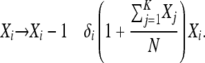
We consider a haploid population composed of K allelic types. The number of each type changes as the result of stochastic birth and death events in continuous time. Each type i is characterized by its intrinsic birth rate, β_i, and death rate, δ_i. Instead of a deterministic population size, the total population number is stochastic and governed by density dependence in the death rates. We further allow offspring from type i to mutate to type j at rate μ_ij; we assume mutations are rare; i.e., 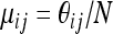. We call this model the generalized Moran process, and we represent it by a Markov chain in which X_i, the number of individuals of type i, has transition rates

(1)

(2)

The parameter N determines the typical population size, as discussed below. This birth–death process is perhaps the simplest possible model of types competing in a population whose size is regulated internally.

Quasi-neutrality:

We focus on the case when the ratio of the intrinsic death rate to the birth rate is the same for each allele, so that

(3)

Although one type may have an elevated birth rate, this is compensated by a correspondingly elevated death rate. We call this case “quasi-neutral”: were the total population size to be held fixed at N_fix by some exogenous mechanism, all individuals would have the same expected lifetime reproductive output [i.e., reproductive value (Fisher 1958; Lande 1982; Charnov 1986)] and equal variance in their lifetime reproductive successes, equal to

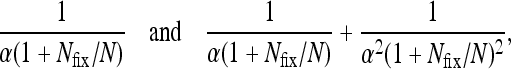respectively [more generally, under this assumption, the moment-generating function for the number of offspring is M(t) = 1 + (e^t − 1)/(α(1 + N_fix/N) + e^t − 1), which is type-independent]. We emphasize that in our model, the total population size varies stochastically, with the consequence that the different types are not in general exchangeable (Cannings 1974).

ANALYTICAL APPROACH

We analyze the generalized Moran process by considering three phases, according to the size of X_i(t). In the first phase, describing the behavior at small initial numbers, we approximate the process by a linear birth–death process with Malthusian growth rate β_i − δ_i. The second phase describes the dynamics at intermediate numbers, for which the abundance of each type, rescaled by N, is asymptotically equivalent to a deterministic system of Gause–Lotka–Volterra equations for logistic growth. The third phase describes the long-term stochastic behavior of the process near carrying capacity; the relative abundance of each type, when time is measured in units proportional to N, converges to a diffusion process as N approaches infinity. The first two limits are valid for all values of β_i and δ_i, while the third exists only when the quasi-neutral condition (3) holds to O(1/N) (for clarity of exposition, we restrict our attention to the case when it holds exactly). These three phases are illustrated in Figure 1 and discussed in greater detail below.

Figure 1.—

Illustrative sample paths of the generalized Moran process. The three distinct phases described by our analytic approximations are indicated (see analytical approach). Dashed lines show solutions to Equations 4 and 5.

Birth–death approximation (phase one):

For 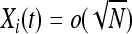and N large, density-dependent and mutational terms in (1) and (2) are o(1) and may be neglected, so X_i(t) may be approximated by a birth–death process with birth rate β_iX_i and death rate δ_iX_i, for which

(4)

A coupling argument (Andersson and Djehiche 1998; Lindvall 2002) may be used to prove convergence almost surely of the generalized Moran process to this birth–death process. Note that this approximation fails when the total population size is ≥, as the density-dependent component of mortality, which is proportional to , may be ≥O(1) and will not vanish with increasing N.

Deterministic approximation (phase two):

For X_i(t) = O(N), we let

where the limit is in probability. Then, Y_i(t) satisfies the deterministic system of ordinary differential equations,

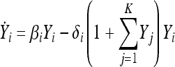(5)

(see Ethier and Kurtz 1986, Chap. 11, Theorem 2.1). We observe that the rates of mutation are O(1/N) and vanish in this limit; i.e., mutational effects can be ignored in the transient dynamics.

When one type has a strictly greater expected reproductive output, i.e.,

(6)

for all j ≠ i, that type rapidly sweeps to fixation for N large (Parsons and Quince 2007). However, in the quasi-neutral case Equation 5 has equilibria at all points such that 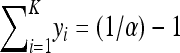, so that, in the infinite-population limit, we would expect coexistence of all types.

Diffusion approximation (phase three):

On a longer timescale, we consider the relative abundances of each type for large N,

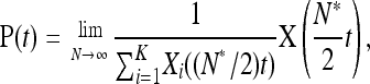where N^* = N(1/α − 1) is the shared carrying capacity.

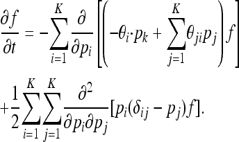
P(t) is a diffusion process whose probability density f(t, p) obeys a forward Kolmogorov equation

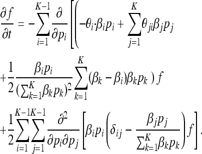(7)

Here, θ_ij = N*μ_ij and 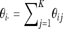. The generator for P(t) is obtained from the generator of X(t) by applying Itô's formula (Protter 2004) to

Convergence to a diffusion follows by arguments similar to those in Ethier and Kurtz (1986, Chap. 11), as described in an associated preprint (Parsons 2010). We also refer to Durrett and Popovic (2009) for a similar argument, in which the initial process is a diffusion rather than a Markov chain; see also Katzenberger (1991). The diffusion equation above is used to obtain the analytical results summarized in Table 1 below. These analytical results are then illustrated in Figures 3 and 4, below, along with comparisons to exact numerical simulations.

TABLE 1.

A comparison of the neutral Wright–Fisher model and the quasi-neutral generalized Moran model

	Wright–Fisher	Generalized Moran
Fixation probability, π(p)	p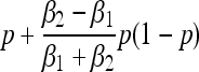
Absorption time
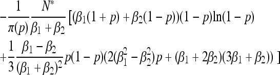
Fixation time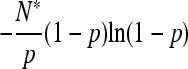
Stationary distribution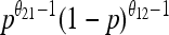

Our analytical, asymptotic results for the generalized Moran model are summarized, which are derived in the main text. Absorption and fixation times are given in generations. For the generalized Moran model the generation time is the average time to reproduction, 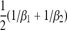, and the carrying capacity is N^* = N(1/α − 1). p is the proportion of type one in a population starting from carrying capacity.

Figure 3.—

(A) The probability that type one fixes, as a function of its initial proportion, for the Wright–Fisher model (blue line) and the generalized Moran model (exact numerical results, solid red line; analytical results from Table 1, dashed black line) starting at carrying capacity. (B) The absorption time of type one under the Wright–Fisher model (blue line) and the generalized Moran model (exact numerical results, solid red line; analytical results from Table 1, dashed black line). Parameter values: β₁ = 2, β₂ = 1, α = 0.5, and N = 1000.

Figure 4.—

The stationary distribution of allele frequencies under reversible mutation. Bars show results from Monte Carlo simulations of the quasi-neutral generalized Moran process (N = 1000, α = 0.5, β₁ = 1.6, β₂ = 2, and μ = 0.0005), in frequency bins of size 10%. Dots show our analytic approximation to the quasi-neutral process, taken from the equation in Table 1. The analytical approximation closely matches the numerical simulation. In addition, the quasi-neutral frequency spectrum is very similar to the spectrum produced by a Wright–Fisher model with selection (triangles). The parameters of a best-fit Wright–Fisher model (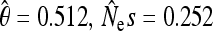) were obtained by applying standard maximum-likelihood inference techniques (Sawyer and Hartl 1992; Bustamante et al. 2001; Desai and Plotkin 2008) to the simulated data, and they would indicate selection favoring the type with low birth rate.

It is important to note that when β_i = β_j = 1 for all i, j (i.e., when all types are strictly neutral), this diffusion equation above simplifies to the standard diffusion for a Wright–Fisher process:

The first and final terms of (7) correspond to mutation and genetic drift, and they agree with the standard diffusion equation of a Wright–Fisher process. In the quasi-neutral regime, however, for each type i there is an additional advective term in (7),

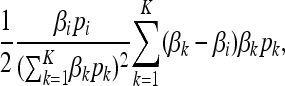proportional to the variation of that type. This term results in an effective selection coefficient favoring the type with lowest birth and death rate, when the population is near carrying capacity.

Results for two types:

When K = 2, P(t) is a diffusion on [0, 1], and we need consider only the proportion of type one, which we denote p.

In the absence of mutation (θ_ij ≡ 0 for all i, j) the boundaries p = 0 and p = 1 are absorbing. Starting from initial frequency p, we study the mean first absorption time, T(p), the probability of fixation of type one, π(p), and the expected time to fixation of type one (i.e., the absorption time conditioned on type one fixing), T₁(p). These quantities satisfy ordinary differential equations related to the forward Kolmogorov Equation (7) (Ewens 2004):

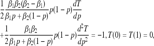and

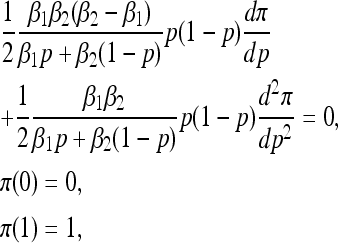and

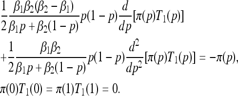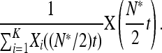
In the presence of mutation (θ_ij > 0), the boundary is no longer absorbing and P(t) has a stationary distribution, which can be expressed as the solution to

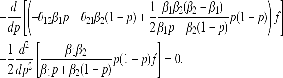(8)

(Ewens 2004). For finite N, the generalized Moran model has only one absorbing state, corresponding to extinction of all types. However, the time to global extinction is exponential in N (and thus tends to infinity as N → ∞). Prior to extinction, the generalized Moran model approaches a quasi-stationary distribution for which the relative frequencies are asymptotically distributed according to the solution of (8).

Expressions for π(p), T(p), and T₁(p) obtained by solving the differential equations above are summarized in Table 1. See, e.g., Ewens (2004) for methods of solution.

NUMERICAL METHODS

The figures below show numerical results for the fixation probabilities and times, along with the analytical approximations derived in the previous section. The numerical results were obtained by solving, via a numerical library for sparse matrices (Davis 2004), the matrix equations for the fixation probabilities and times as formulated from the transition rates (1) and (2) (Stewart 1994). The number of possible states is unbounded so it was necessary to apply a truncation T on the maximum population number of both types. It was found that as the truncation point was moved beyond the carrying capacity N*, numerical results for fixation times or probabilities starting from states around or below this point converged to within machine precision by T = 1.5N*; consequently this value was used.

RESULTS

Figure 2 shows an illustrative sample path of the generalized Moran process, starting from a small population, obtained by Monte Carlo simulation. Initially, the number of each type grows exponentially, and the type with higher birth and death rates grows faster. Over the long term, however, the total population size stabilizes near its carrying capacity, and the type with the lower birth and death rates dominates, because it is less prone to fluctuation. Thus, it appears that selection initially favors type one and subsequently favors type two—a phenomenon that we explore in greater detail below.

Figure 2.—

An illustrative stochastic realization of the generalized Moran process, starting from a population composed of 10 individuals of each type. Initially, the type with the high birth and death rates grows faster (top), but over the long term the type with low birth and death rates dominates (bottom). The two types have the same expected lifetime reproductive output, and they would behave neutrally in a standard Wright–Fisher model with fixed population size. The two panels show output from the same simulation, with different scales on the time axis. Parameters values: β₁ = 2, β₂ = 1, α = 0.5, N = 1000, and μ₁₂ = μ₂₁ = 0.01.

We have developed a rigorous analytical framework for studying the dynamics of the generalized Moran model (see analytical approach). As our analysis shows, the behavior illustrated in Figure 2 arises because the population size is not deterministic. The total population size will quickly approach and thereafter fluctuate around the common carrying capacity N^* = (1 − (1/α))N. Given, as we observed above, the two types have equal expected lifetime output at fixed population size, one might therefore suspect that the classical quantities, such as the probability and mean time before fixation of a mutant allele, would be given by their neutral Wright–Fisher expectation with an effective population size N_e = N*/2. This is false, however. When two quasi-neutral types differ substantially in their vital rates (i.e., by order one), then there is no effective population size, including the harmonic mean (Ewens 1967; Otto and Whitlock 1997), for which the behavior of the stochastic population is captured by a Wright–Fisher diffusion—even if the population is started from carrying capacity (see analytical results in Table 1).

Under the Wright–Fisher model without mutation, a neutral allele will fix with probability given by its initial frequency. In the generalized Moran model, however, the fixation probability differs qualitatively from the Wright–Fisher expectation (Table 1). Starting from a population at carrying capacity, the fixation probability of a mutant has a quadratic dependence on the mutant's initial frequency, and it favors fixation of the type with low birth and death rates (Figure 3a). Differences in generation time induce a form of apparent selection favoring one type over another—despite the fact that the two types would appear to be strictly neutral variants under a Wright–Fisher model with N_e = N*/2.

A similar result holds for the mean time before a mutant allele fixes or goes extinct. The behavior of the generalized Moran process is skewed relative to the neutral Wright–Fisher prediction: the mean absorption time is longer than the classical expectation when the type with higher birth rate forms a larger initial proportion of the population (Figure 3b). The conditional mean time before fixation of an allele is also skewed: the type with low vital rates fixes more quickly than a type with high vital rates. Again, the generalized Moran model exhibits a form of selection that favors one type over another, despite the fact that the two types would have the same expected lifetime reproductive output were the population size held fixed at N*.

When mutations are permitted between the two types, then the population, conditioned on nonextinction, will reach a stationary state determined by a balance of mutation and drift. For the neutral Kimura diffusion with effective population size N_e = (N^*/2), when mutation rates are symmetric (i.e., μ₁₂ = μ₂₁ = μ), the stationary relative frequency, p, of type one follows the well-known beta distribution

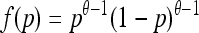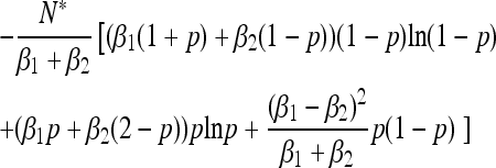
(Ewens 2004), where θ = 2N_eμ. For a quasi-neutral stochastic population, by contrast, the stationary distribution of type one is given by the solution to (8):

(9)

As we demonstrate below, the stationary allele frequency distribution of the generalized Moran process (Equation 9) is very similar to that of a Wright–Fisher model with selection favoring the type with low birth rate.

All of the analytical results summarized in Table 1 are asymptotic in N. These asymptotic approximations are highly accurate for N = 1000, as demonstrated in Figures 3 and 4, and therefore also for N > 1000.

PRACTICAL IMPLICATIONS

The results above have important consequences for practitioners who wish to make inferences about natural selection on the basis of samples from wild or laboratory populations. When life-history traits are under genetic control, inference based on standard assumptions (i.e., Kimura's diffusion) may yield erroneous and even contradictory conclusions: at small population densities one allele will appear superior, whereas at large densities the other allele will dominate. We illustrate this point using two examples of the types of inferences typically drawn from population data.

In the first example, we analyzed polymorphism “data” generated by simulating the generalized Moran processes of competing, quasi-neutral types. We sampled 100 individuals from a large population near carrying capacity, and we recorded the polymorphism frequency spectrum across 1000 independent sites (Figure 4). The observed spectrum, which describes the number of sites at which the type-one allele segregates at different frequencies, is typical of the polymorphism data observed in field studies of microbes and higher eukaryotes (e.g., Hartl et al. 1994; Akashi and Schaeffer 1997). If we analyze the simulated polymorphism data using standard inference techniques based on the Wright–Fisher diffusion (Sawyer and Hartl 1992; Bustamante et al. 2001; Desai and Plotkin 2008), we would infer directional selection favoring the type with low birth rate (Figure 4).

This result is important because alternative approaches to inferring selection pressures from data would reach the opposite conclusion. Selection coefficients are often quantified by competing two types in a nutrient-rich laboratory environment and measuring the difference in their initial exponential growth rates (Lenski et al. 1991; Lenski and Elena 2003). Under the generalized Moran model starting from a small population, type one will grow at exponential rate β₁ − δ₁ = β₁(1 − α) and type two at exponential rate β₂ − δ₂ = β₂(1 − α), yielding an apparent selective advantage to the type with high birth rate. Thus, the selection coefficient inferred from a laboratory competition experiment will have the opposite sign to the selection coefficient inferred from the stationary polymorphism frequency spectrum, as would be sampled in the field.

To take a textbook example, in a 12-hr competition experiment from small initial numbers the frequency of Escherichia coli strain gnd(RM77C) increased from 0.455 to 0.898, relative to strain gnd(RM43A) (Hartl and Dykhuizen 1981). The standard interpretation of these data suggests that strain RM77C is selectively advantageous (N_es = 0.067) and that it will eventually fix with a probability greater than its frequency at 12 hr (Hartl and Clark 2006). But these data are equally compatible with the quasi-neutral generalized Moran model, which predicts that RM77C will be disadvantageous when the population eventually reaches carrying capacity and that it will fix with a probability less than its frequency at 12 hr. Thus, the interpretation of such a competition experiment depends on the trade-offs that occur between birth rate and other life-history traits and also on assumptions about the underlying demographic process.

Our results also have implications for serial transfer experiments used to study microbial evolution (e.g., Lenski et al. 1991; Bull et al. 1997; Holder and Bull 2001). In Figure 5 we consider the generalized Moran process with the addition of periodic bottlenecks in the population size, representative of periodic transfers. Fixation probabilities for the process with bottlenecks were obtained via Monte Carlo simulations. In this case, the probability that one quasi-neutral type will fix as opposed to another depends on the bottleneck frequency: when bottlenecks are infrequent, the type with low birth rate is more likely to fix, whereas the opposite occurs when bottlenecks are frequent. This result implies that the choice of serial transfer protocol induces a form of selection for one or another life-history phenotype, according to the transfer frequency—a phenomenon that should be considered when designing and interpreting laboratory studies of microbial evolution.

Figure 5.—

Bottleneck frequency influences fixation probability under the quasi-neutral generalized Moran model (red circles), but not under the neutral Wright–Fisher model (blue dashed line). Simulated populations were initiated at carrying capacity with an equal number of individuals of type one and type two. The populations were then periodically bottlenecked to 10 individuals, by binomial sampling. When bottlenecks are frequent, the type with larger birth rate is more likely to fix and conversely when bottlenecks are infrequent. Parameter values: N = 1000, α = 0.5, β₁ = 0.4, and β₂ = 2.

Previous work on life history has reached similar conclusions about fixation probabilities. For example, Alexander and Wahl (2008) found that two different beneficial mutations with the same expected lifetime reproductive output may have different fixation probabilities relative to a disadvantageous wild type. However, such analyses were based on a branching process approximation that applies only in the limit of strong selection, when the fixation of the mutant is ensured once it escapes genetic drift (Wahl and Gerrish 2001; Wahl and Dehaan 2004; Alexander and Wahl 2008). By contrast, we have demonstrated that an invading mutant may be favored or disfavored compared to wild type, depending on the population size when it is introduced or the frequency of bottlenecks.

DISCUSSION

Here we have studied a simple stochastic model of births and deaths in continuous time, which is more realistic than the Wright–Fisher model in many circumstances. We have derived analytic expressions for fixation probabilities, absorption times, and steady-state polymorphism distributions. We find that when the population size is near carrying capacity, one type is preferred, and when far from carrying capacity, the other type is preferred—despite the fact that both types have the same expected lifetime reproductive output. These results have implications for our understanding of molecular evolution and for the interpretation of evolutionary studies in the field and in the laboratory.

The behavior of the generalized Moran process in the quasi-neutral regime can be understood as a form of r-vs.-K selection (Pianka 1972; MacArthur and Wilson 2001). Quasi-neutrality enforces a life-history trade-off in which an increased birth rate is compensated by an increased death rate. The type with the lower mortality rate is favored when the population size is large (i.e., near carrying capacity), because such a type experiences less dramatic fluctuations and is less likely to go extinct. As a result, fixation probabilities, absorption times, and the stationary polymorphism frequency spectrum favor the type with low birth rate. In contrast, when the total population size is small, so that density-dependent regulation is weak, rapid growth is preferable and the type with higher birth rate is favored. Thus, in a model with stochastic population size there is no one-dimensional “selection coefficient” that summarizes the dynamics of competing types (see also Lambert 2005, 2006; Champagnat and Lambert 2007).

A trade-off between mortality and fecundity may be interpreted as a form of evolutionary bet hedging (Slatkin 1974), where high-fecundity strategies produce greater variability in lifetime reproductive success, but they are selectively disadvantageous in saturated environments. Similar results have previously been observed by Gillespie and others, who studied models in which individuals produce variable numbers of offspring (Gillespie 1974, 1975, 1977; Proulx 2000; Shpak 2007). Like the generalized Moran model, such models are not equivalent to a Wright–Fisher diffusion, for any constant value of the effective population size. Nonetheless, our results differ from those of Gillespie, who assumed that the population size is held constant by some exogenous mechanism. We have shown that these effects arise in populations that are intrinsically regulated by density dependence. Indeed, differences in individual fecundity variance appear only when the total population size is allowed to vary. Moreover, when the population size is stochastic, one type will be favored at low density and another type at high density. Combined with exogenous disturbances, these effects can drastically change the probability of fixation (e.g., Figure 5).

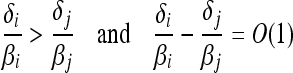
Quasi-neutrality is a novel phenomenon that arises when the total population number is allowed to vary stochastically, in a hybrid regime between strong and weak selection. When one type has a significantly greater lifetime reproductive success [i.e., β_i/δ_i > β_i/δ_i+O(1)], then that type will sweep with probability approaching one as the carrying capacity becomes large. By contrast, when the birth and death rates differ by a small amount [ and ], we recover the classical theory of weak selection. Quasi-neutrality arises in an intermediate regime: when two or more types have overall reproductive success that differs by at most , achieved through birth and death rates that differ by O(1).

Since quasi-neutrality occurs in a limited regime of parameters, the question arises as to whether this regime is found in natural populations. After all, any mutations that confer a significant improvement in overall reproductive success will quickly displace neutral or quasi-neutral segregating types. Indeed, such arguments have been raised against the biological relevance of Gillespie's model (e.g., Hopper et al. 2003 and references therein), which operates in a similar parameter regime. Nevertheless, there are both theoretical and empirical reasons why quasi-neutral types might regularly segregate in populations—arguments analogous to those that support widespread neutral variation. In a fixed environment, mutations that confer strong selective advantages will fix quickly and be depleted (Lenski and Travisano 1994); and so eventually most segregating variation will be neutral, weakly selected, or quasi-neutral. Once strongly selected mutations have been exhausted, any mutations that allow an organism to vary its allocation to reproduction vs. survivorship will begin to segregate. Thus, quasi-neutral types will most likely segregate in depleted or subdivided environments where the carrying capacity of a given patch is small (Shpak 2005) or in populations where most mutations that convey an absolute fitness advantage have already fixed.

We have focused on the quasi-neutral case, to highlight the contrast between the generalized Moran process and the standard, neutral Wright–Fisher diffusion. Nevertheless, our analysis extends to competing types with different expected reproductive outputs—i.e., values of that differ by (Parsons 2010). In other words, the r-vs.-K dynamic we have observed also operates in the presence of traditional forms of weak selection.

Fecundity/mortality trade-offs of the broad type we have considered here may be ubiquitous in microorganisms, arising from multiple alternative mechanisms. Such trade-offs have been observed empirically in E. coli subject to prolonged starvation: lower intrinsic mortality rates allowed adapted strains to persist in minimal salts media, but such strains proved to be inferior competitors in fresh medium (Vasi and Lenski 1999). Trade-offs between phage resistance and growth rate—arising because resistance involves the loss of receptors on the cell surface that are both exploited by the phage to gain entry and involved in the uptake of nutrients—are also well documented (Bohannan and Lenski 2000; Bohannan et al. 2002). Similarly, antibiotic resistance often causes a reduction in doubling time, because of the costs of actively transporting the antibiotic out of the cell through efflux pumps, e.g., in fluoroquinolone resistance in Salmonella enterica (Giraud et al. 2003). The exact shape of these trade-offs may differ from the linear one considered here (Jessup and Bohannan 2008), and our population dynamics—with demographic rates that depend linearly on population number—will apply only as an approximation. Nonetheless, the potential exists for conditions analogous to quasi-neutrality, such that the corresponding deterministic model of competition predicts stable coexistence. Indeed, empirical studies of E. coli strains competing in a chemostat (Hansen and Hubbell 1980) under just these conditions have produced time series in which one type predominates at low density but is then less abundant in saturated media, much as our model predicts (Figure 2). Consequently the phenomena we have investigated, i.e., stochastic contributions to the fitness of competing types, may be important in shaping patterns of microbial genetic diversity.

References

- Akashi, H., and S. W. Schaeffer, 1997. Natural selection and the frequency distributions of “silent” DNA polymorphism in Drosophila. Genetics 146 295–307. [DOI] [PMC free article] [PubMed] [Google Scholar]
- Alexander, H. K., and L. M. Wahl, 2008. Fixation probabilities depend on life history: fecundity, generation time and survival in a burst-death model. Evolution 62 1600–1609. [DOI] [PubMed] [Google Scholar]
- Andersson, H., and B. Djehiche, 1998. A threshold limit theorem for the stochastic logistic epidemic. J. Appl. Probab. 35 662–670. [Google Scholar]
- Bohannan, B. J. M., and R. E. Lenski, 2000. Linking genetic change to community evolution: insights from studies of bacteria and bacteriophage. Ecol. Lett. 3 362–377. [Google Scholar]
- Bohannan, B. J. M., B. Kerr, C. M. Jessup, J. B. Hughes and G. Sandvik, 2002. Trade-offs and coexistence in microbial microcosms. Antonie Van Leeuwenhoek 81 107–115. [DOI] [PubMed] [Google Scholar]
- Bull, J. J., M. R. Badgett, H. A. Wichman, J. P. Huelsenbeck, D. M. Hillis et al., 1997. Exceptional convergent evolution in a virus. Genetics 147 1497–1507. [DOI] [PMC free article] [PubMed] [Google Scholar]
- Bustamante, C. D., J. Wakeley, S. Sawyer and D. L. Hartl, 2001. Directional selection and the site-frequency spectrum. Genetics 159 1779–1788. [DOI] [PMC free article] [PubMed] [Google Scholar]
- Cannings, C., 1974. The latent roots of certain Markov chains arising in genetics: a new approach, i. haploid models. Adv. Appl. Probab. 6 260–290. [Google Scholar]
- Champagnat, N., and A. Lambert, 2007. Evolution of discrete populations and the canonical diffusion of adaptive dynamics. Ann. Appl. Probab. 17 102–155. [Google Scholar]
- Charnov, E. L., 1986. Dimensionless numbers and life history evolution: age of maturity versus the adult lifespan. Evol. Ecol. 4 273–275. [Google Scholar]
- Davis, T. A., 2004. Algorithm 832: UMFPACK, an unsymmetric-pattern multifrontal method. ACM Trans. Math. Soft. 30 196–199. [Google Scholar]
- Desai, M. M., and J. B. Plotkin, 2008. The polymorphism frequency spectrum of finitely many sites under selection. Genetics 180 2175–2191. [DOI] [PMC free article] [PubMed] [Google Scholar]
- Donnelly, P., 1986. A genealogical approach to variable-population-size models in population genetics. J. Appl. Probab. 23 283–296. [Google Scholar]
- Durrett, R., 2009. Probability Models for DNA Sequence Evolution, Ed. 2. Springer, New York.
- Durrett, R., and L. Popovic, 2009. Degenerate diffusions arising from gene duplication models. Ann. Appl. Probab. 19 15–48. [Google Scholar]
- Ethier, S. N., and T. G. Kurtz, 1986. Markov Processes: Characterization and Convergence. Wiley Interscience, Hoboken, NJ.
- Ewens, W. J., 1967. The probability of survival of a new mutant in a fluctuating environment. Heredity 22 438–443. [DOI] [PubMed] [Google Scholar]
- Ewens, W. J., 1972. The sampling theory of selectively neutral alleles. Theor. Popul. Biol. 3 87–112. [DOI] [PubMed] [Google Scholar]
- Ewens, W. J., 2004. Mathematical Population Genetics, Ed. 2. Springer, New York.
- Fay, J. C., and C.-I. Wu, 2000. Hitchhiking under positive Darwinian selection. Genetics 155 1405–1413. [DOI] [PMC free article] [PubMed] [Google Scholar]
- Fisher, R. A., 1958. The Genetical Theory of Natural Selection. Dover, New York.
- Fu, Y. X., and W. H. Li, 1992. Statistical tests of neutrality of mutations. Genetics 133 693–709. [DOI] [PMC free article] [PubMed] [Google Scholar]
- Gause, G. F., 1934. The Struggle for Existence. Williams & Watkins, Baltimore.
- Gillespie, J. H., 1974. Nautural selection for within-generation variance in offspring number. Genetics 76 601–606. [DOI] [PMC free article] [PubMed] [Google Scholar]
- Gillespie, J. H., 1975. Natural selection for within-generation variance in offspring number ii. discrete haploid models. Genetics 81 403–413. [DOI] [PMC free article] [PubMed] [Google Scholar]
- Gillespie, J. H., 1977. Natural selection for variances in offspring numbers: a new evolutionary principle. Am. Nat. 111 1010–1014. [Google Scholar]
- Giraud, E., A. Cloeckaert, S. Baucheron, C. Mouline and E. Chaslus-Dancla, 2003. Fitness cost of fluoroquinolone resistance in Salmonella enterica serovar Typhimurium. J. Med. Microbiol. 52 697–703. [DOI] [PubMed] [Google Scholar]
- Griffiths, R. C., and S. Tavaré, 1994. Sampling theory for neutral alleles in a varying environment. Philos. Trans. R. Soc. Lond. B 344 403–410. [DOI] [PubMed] [Google Scholar]
- Hansen, S. R., and S. P. Hubbell, 1980. Single-nutrient microbial competition: qualitative agreement between experimental and theoretically forecast outcomes. Science 207 1491–1493. [DOI] [PubMed] [Google Scholar]
- Hartl, D. L., and A. G. Clark, 2006. Principles of Population Genetics, Ed. 4. Sinauer Associates, Sunderland, MA.
- Hartl, D. L., and D. E. Dykhuizen, 1981. Potential for selection among nearly neutral allozymes of 6-phosphogluconate dehydrogenase in Escherichia coli. Proc. Natl. Acad. Sci. USA 78 6344–6348. [DOI] [PMC free article] [PubMed] [Google Scholar]
- Hartl, D. L., E. N. Moriyama and S. A. Sawyer, 1994. Selection intensity for codon bias. Genetics 138 227–234. [DOI] [PMC free article] [PubMed] [Google Scholar]
- Holder, K. K., and J. J. Bull, 2001. Profiles of adaptation in two similar viruses. Genetics 159 1393–1404. [DOI] [PMC free article] [PubMed] [Google Scholar]
- Hopper, K., J. Rosenheim, T. Prout and S. Oppenheim, 2003. Within-generation bet hedging: A seductive explanation? Oikos 101 219–222. [Google Scholar]
- Hudson, R. R., M. Kreitman and M. Aguadé, 1987. A test of neutral molecular evolution based on nucleotide data. Genetics 116 153–159. [DOI] [PMC free article] [PubMed] [Google Scholar]
- Jessup, C. M., and B. J. M. Bohannan, 2008. The shape of an ecological trade-off varies with environment. Ecol. Lett. 11 947–959. [DOI] [PubMed] [Google Scholar]
- Kaj, I., and S. M. Krone, 2003. The coalescent process in a population with stochastically varying size. J. Appl. Probab. 40 33–48. [Google Scholar]
- Karlin, S., and J. McGregor, 1964. Direct product branching processes and related Markov chains. Proc. Natl. Acad. Sci. USA 51 598–602. [DOI] [PMC free article] [PubMed] [Google Scholar]
- Katzenberger, G. S., 1991. Solutions of a stochastic differential equation forced onto a manifold by a large drift. Ann. Probab. 19 1587–1628. [Google Scholar]
- Kimura, M., 1955. Solution of a process of random genetic drift with a continuous model. Proc. Natl. Acad. Sci. USA 41 144–150. [DOI] [PMC free article] [PubMed] [Google Scholar]
- Kimura, M., 1962. On the probability of fixation of mutant genes in a population. Genetics 47 713–719. [DOI] [PMC free article] [PubMed] [Google Scholar]
- Kimura, M., and T. Ohta, 1974. Probability of gene fixation in an expanding finite population. Proc. Natl. Acad. Sci. USA 71 3377–3379. [DOI] [PMC free article] [PubMed] [Google Scholar]
- Kingman, J. F. C., 1982. The coalescent. Stoch. Proc. Appl. 13 235–248. [Google Scholar]
- Lambert, A., 2005. The branching process with logistic growth. Ann. Appl. Probab. 69 419–441. [Google Scholar]
- Lambert, A., 2006. Probability of fixation under weak selection: a branching process unifying approach. Theor. Popul. Biol. 15 1506–1535. [DOI] [PubMed] [Google Scholar]
- Lande, R., 1982. A quantitative genetic theory of life history evolution. Ecology 63 607–615. [Google Scholar]
- Lenski, R., and S. F. Elena, 2003. Evolution experiments with microorganisms: the dynamics and genetic bases of adaptation. Nat. Rev. Genet. 4 457–469. [DOI] [PubMed] [Google Scholar]
- Lenski, R., M. R. Rose, S. Simpson and S. C. Tadler, 1991. Long-term experimental evolution in Escherichia coli i. Am. Nat. 138 1315–1341. [Google Scholar]
- Lenski, R. E., and M. Travisano, 1994. Dynamics of adaptation and diversification: a 10,000-generation experiment with bacterial populations. Proc. Natl. Acad. Sci. USA 91 6808–6814. [DOI] [PMC free article] [PubMed] [Google Scholar]
- Lessard, S., 2007. An exact sampling formula for the Wright–Fisher model and a solution to a conjecture about the finite-island model. Genetics 177 1249–1254. [DOI] [PMC free article] [PubMed] [Google Scholar]
- Lindvall, T., 2002. Lectures on the Coupling Method. Dover, Mineola, NY.
- Lotka, A. J., 1925. Elements of Physical Biology. Williams & Watkins, Baltimore.
- MacArthur, R. H., and E. O. Wilson, 2001. The Theory of Island Biogeography. Princeton University Press, Princeton, NJ.
- McDonald, J., and M. Kreitman, 1991. Adaptive protein evolution at the Adh locus in Drosophila. Nature 351 652–654. [DOI] [PubMed] [Google Scholar]
- Möhle, M., 2001. Forward and backward diffusion approximations for haploid exchangeable population models. Stoch. Proc. Appl. 95 133–149. [Google Scholar]
- Moran, P. A. P., 1958. Random processes in genetics. Proc. Camb. Philos. Soc. 54 60–71. [Google Scholar]
- Otto, S. P., and M. C. Whitlock, 1997. The probability of fixation in populations of changing size. Genetics 146 723–733. [DOI] [PMC free article] [PubMed] [Google Scholar]
- Parsons, T. L., 2010. Limit theorems for competitive density dependent population processes. arXiv, http://arxiv.org/abs/1005.0010.
- Parsons, T. L., and C. Quince, 2007. Fixation in haploid populations exhibiting density dependence I: the non-neutral case. Theor. Popul. Biol. 72 121–135. [DOI] [PubMed] [Google Scholar]
- Pascual, M. A., and P. Kareiva, 1996. Predicting the outcome of competition using experimental data: maximum likelihood and Bayesian approaches. Ecology 77 337–349. [Google Scholar]
- Pianka, E. R., 1972. r and K selection or b and d selection? Am. Nat. 106 581–588. [Google Scholar]
- Protter, P. E., 2004. Stochastic Integration and Differential Equations, Ed. 2. Springer, Berlin.
- Proulx, S. R., 2000. The ESS under spatial variation with applications to sex allocation. Theor. Popul. Biol. 58 33–47. [DOI] [PubMed] [Google Scholar]
- Sawyer, S. A., and D. L. Hartl, 1992. Population genetics of polymorphism and divergence. Genetics 132 1161–1176. [DOI] [PMC free article] [PubMed] [Google Scholar]
- Shpak, M., 2005. Evolution of variance in offspring number: the effects of population size and migration. Theor. Biosci. 124 65–85. [DOI] [PubMed] [Google Scholar]
- Shpak, M., 2007. Selection against demographic stochasticity in age-structured populations. Genetics 177 2181–2194. [DOI] [PMC free article] [PubMed] [Google Scholar]
- Slatkin, M., 1974. Hedging one's evolutionary bets. Nature 250 704–705. [Google Scholar]
- Stewart, W. J., 1994. Introduction to the Numerical Solution of Markov Chains. Princeton University Press, Princeton, NJ.
- Tajima, F., 1989. Statistical method for testing the neutral mutation hypothesis by DNA polymorphism. Genetics 123 585–595. [DOI] [PMC free article] [PubMed] [Google Scholar]
- Taylor, J. E., 2009. The genealogical consequences of fecundity variance polymorphism. Genetics 182 813–837. [DOI] [PMC free article] [PubMed] [Google Scholar]
- Vandermeer, J. H., 1969. The competitive structure of communities: an experimental approach with protozoa. Ecology 50 362–371. [Google Scholar]
- Vasi, F. K., and R. E. Lenski, 1999. Ecological strategies and fitness tradeoffs in Escherichia coli mutants adapted to prolonged starvation. J. Genet. 78 43–49. [Google Scholar]
- Volterra, V., 1926. Fluctuations in the abundance of a species considered mathematically. Nature 118 558–560. [Google Scholar]
- Wahl, L. M., and C. S. DeHaan, 2004. Fixation probability favors increased fecundity over reduced generation time. Genetics 168 1009–1018. [DOI] [PMC free article] [PubMed] [Google Scholar]
- Wahl, L. M., and P. J. Gerrish, 2001. Fixation probability in populations with periodic bottlenecks. Evolution 55 2606–2610. [DOI] [PubMed] [Google Scholar]
- Wakeley, J., 2005. The limits of theoretical population genetics. Genetics 169 1–7. [DOI] [PMC free article] [PubMed] [Google Scholar]
- Wakeley, J., 2009. Coalescent Theory: An Introduction. Roberts & Co., New York.
- Wright, S., 1931. Evolution in Mendelian populations. Genetics 16 97–159. [DOI] [PMC free article] [PubMed] [Google Scholar]
- Yang, Z., and J. P. Bielawski, 2000. Statistical methods for detecting molecular adaptation. Trends Ecol. Evol. 15 496–503. [DOI] [PMC free article] [PubMed] [Google Scholar]