

Abstract
We present and evaluate a rigid-body molecular docking method, called PATIDOCK, that relies solely on the three-dimensional structure of the individual components and the experimentally derived residual dipolar couplings (RDC) for the complex. We show that, given an accurate ab initio predictor of the alignment tensor from a protein structure, it is possible to accurately assemble a protein-protein complex by utilizing the RDC’s sensitivity to molecular shape to guide the docking. The proposed docking method is robust against experimental errors in the RDCs and computationally efficient. We analyze the accuracy and efficiency of this method using experimental or synthetic RDC data for several proteins, as well as synthetic data for a large variety of protein-protein complexes. We also test our method on two protein systems for which the structure of the complex and steric-alignment data are available (Lys48-linked diubiquitin and a complex of ubiquitin and a ubiquitin-associated domain) and analyze the effect of flexible unstructured tails on the outcome of docking. The results demonstrate that it is fundamentally possible to assemble a protein-protein complex based solely on experimental RDC data and the prediction of the alignment tensor from three-dimensional structures. Thus, despite the purely angular nature of residual dipolar couplings, they can be converted into intermolecular distance/translational constraints. Additionally we show a method for combining RDCs with other experimental data, such as ambiguous constraints from interface mapping, to further improve structure characterization of the protein complexes.
Introduction
Detailed understanding of molecular mechanisms underlying biological function requires knowledge of the three-dimensional structure of biomacromolecules and their complexes. Nuclear magnetic resonance (NMR) spectroscopy is one of the main methods for obtaining information on molecular structure and interactions at atomic-level resolution. A major challenge in using NMR for accurate structure determination of multidomain systems and macromolecular complexes is the scarcity of long-distance structural information. Intermolecular Nuclear Overhauser Effect (NOE) contacts are often scarce, difficult to detect, and could be affected by intermolecular motions. Chemical shift perturbation (CSP) mapping is another powerful method for general identification of the interface. However, its informational content is highly ambiguous because CSPs do not identify pair-wise contacts and should be used with caution, since a perturbation of the local electronic environment of a nucleus does not necessarily indicate direct involvement of the corresponding atom in the interactions. Moreover, both NOEs and CSPs are limited to the contact area and could be insufficient for accurate spatial arrangement of the interacting partners. Residual dipolar couplings (RDCs), resulting from partial molecular alignment in a magnetic field,1,2 could supplement the scarce interdomain data, because they contain valuable structural information in terms of global, long-range orientational constraints (reviewed in3). In addition, RDCs also inevitably reflect (hence are sensitive to) the physical properties of the solute molecule responsible for its alignment. Thus, a commonly used method for aligning proteins in solution takes advantage of the anisotropy of molecular shape by imposing steric restrictions on the allowed orientations of the molecule. Such steric alignment can often be modeled as caused by planar obstacles (see e.g.,2,4); we will refer to this simplified model of molecular alignment as the barrier model.
The alignment of a rigid molecule can be characterized by the so-called alignment tensor. Several methods have been developed4–8 to use the barrier model for predicting the alignment tensor (and with it the RDCs) either directly from the 3D shape of the molecule or indirectly, using an ellipsoid representation. The RDCs’ sensitivity to molecular shape has the potential for improving structure characterization, especially in multi-domain systems and macromolecular complexes, by fully integrating RDC prediction into structure refinement protocols to directly drive structure optimization. In fact, RDCs have been used to orient domains and bonds relative to each other either directly, using rigid-body rotation,9–13 or by incorporating RDCs as orientational restraints into protein docking14–16 (see e.g., the reviews17,18). However, none of these methods has used the information on the shape of the molecule (including not only the intervector/interdomain orientation but also the actual positioning of the individual domains) embedded in the measured RDCs.
Another physical property sensitive to molecular shape is the overall rotational diffusion tensor, characterizing the rates and anisotropy of the overall tumbling of a molecule in solution. Interestingly, although they reflect distinct physical phenomena (rotation versus orientation) the diffusion and the alignment tensors are oriented similarly, provided the alignment is caused by neutral planar obstacles.19 As demonstrated recently by Ryabov and Fushman,20 the sensitivity of the overall rotational diffusion tensor to molecular shape can be utilized to guide molecular docking. One would expect that the alignment tensor could be used similarly. Given that accurate RDC measurements for a wide variety of bond vectors are readily available, the use of the alignment tensor to guide molecular assembly could be of significant value for a broad range of macromolecular systems. However, to our knowledge, the ability to dock molecules using the alignment tensor has not been demonstrated, and RDCs have never been used to completely drive molecular docking, i.e. not only orient but also properly position molecules/domains relative to each other in a complex.
In this paper we demonstrate that it is possible to determine the structure of a complex by utilizing the sensitivity of RDCs to molecular shape, provided that the structures of the individual components of the complex are available. We describe a method for rigid-body molecular docking based solely on the orientation- and shape-related information embedded in the experimental RDCs/alignment tensor of the complex. This method, called PATIDOCK, uses a recently developed computationally efficient algorithm (PATI8) for ab initio prediction of the alignment tensor from the three-dimensional shape of a molecule. We demonstrate that PATIDOCK can deterministically and efficiently perform rigid-body docking based on the alignment tensor. In addition, we analyze the robustness of PATIDOCK under certain types of experimental errors, examine its performance in applications to real experimental data, and discuss challenges and various ways of refining the results by including other available experimental restraints and integrating our method into more sophisticated docking approaches.
Methods
Here we present a method, called PATIDOCK, for rigid-body assembly of a molecule made up of two distinct sets of atoms (hereafter called domains) whose structures are known, by using experimental RDC values exclusively. The method is based on first rotating/aligning the two domains using the corresponding subsets of the RDC values (see e.g.,9,11,13) and then translating/positioning them relative to each other in order to minimize the difference between the predicted A and the experimental à alignment tensors. A is computed for the complex using the barrier-model-based algorithm PATI, while à is derived directly from the RDC values, measured for the whole molecule, using a linear least squares approach (see e.g.,8,21) and the (already aligned) 3D structures of the individual domains. As discussed in Berlin et al.,8 PATI predicts RDCs with the same accuracy as program PALES,4 while its computational efficiency is achieved by using numerical integration and a convex hull representation of the molecular surface. Note that while some parts of the docking algorithm are specific to the use of PATI, the general algorithm and key concepts can be applied to any current or future method for alignment tensor prediction.
Formulation
We formulate the docking algorithm as a minimization problem. The algorithm is based on minimizing the difference between the predicted alignment tensor A, computed based on the structure/shape of the molecule, and the experimental alignment tensor Ã, derived directly from the experimental RDC values.
Let the set S of atoms of a molecule be subdivided into two distinct sets (domains), S1 and S2, such that S1 ∩ S2 = ∅, S1 ∪ S2 = S, no RDC-active bond is shared between the two sets, and each set contains enough bond vectors/RDCs associated with it to provide a proper sampling of the orientational space required for accurate determination of the alignment tensors.22 We define A(Rc, x) as the predicted alignment tensor of S, where the coordinates of atoms in S1 remain static and the coordinates of atoms in S2 are rotated by some rotation matrix Rc and then translated by x = [x1, x2, x3]. Our goal is to first properly orient the two sets by finding the optimal rotation matrix, R*, and then to find the optimal translation vector x* that minimizes the difference between A(R*,x) and Ã. The separation of orientation from translation is possible because inter-domain orientation can be obtained directly from the experimental RDCs and bond vectors for each set,9,11,13 regardless of their relative position.
To solve for R* we simply align S1 and S2 relative to each other using experimental RDC data, as described in.9,11,13 We first compute the experimental alignment tensors, Ã1 and Ã2, of S1 and S2, respectively. The alignment tensors have eigendecompositions and , where R1, R2 are rotation matrices (orthogonal matrices with determinant of 1) and D1, D2 are the diagonal matrices of principal components of the corresponding alignment tensors. Therefore, R* can be derived by solving the equation R*R2 = R1:
| (1) |
Note that due to orientational degeneracy of the alignment tensor there is a four-fold ambiguity in the relative alignment of domains, hence four possible solutions for R*.13 One can find these possible solutions by computing an eigendecomposition of Ã2, determining the four assignments of signs to the columns of R2 that make det(R2) = 1, and using Equation (1) for each one. Note that in the case when two or more eigenvalues of the alignment tensor are close to each other (e.g. very low rhombicity) it might not be possible to accurately orient the two domains. In this case additional experimental information, e.g. in the form of interdomain contacts (see below), could come to rescue.
Knowing the optimal rotation matrix R*, we find the optimal translation vector x* by solving a nonlinear least squares problem. Since R* is derived directly from the experimental RDC data independent of x*, in the rest of the paper (except for the last sections) we assume that the two subsets are already properly aligned and simplify the notation from A(Rc, x) to A(x). Our nonlinear least squares problem is then formulated as:
| (2) |
where the target function is defined as
| (3) |
and the computation of A(x) is described in the next section.
Efficient Computation of the Alignment Tensor
In this section we reformulate PATI, from the formulae presented in Berlin et al.,8 to one that can be efficiently recomputed multiple times on S under different translations of S2.
From equations for PATI in Berlin et al.,8 given a set of atoms S and a unit vector b = [b1, b2, b3] in the direction of a static magnetic field, the predicted alignment tensor A of S can be expressed as:
| (4) |
where 2h is the distance between the planar barriers oriented orthogonal to the z axis. η(α,u) is the difference between the z-coordinate of the center of the molecule and the minimum z-coordinate value of all points in S at a given orientation of the molecule, specified by the zyz Euler rotation angles [α, β, γ], and u = cosβ. See the Supporting Material for definition of the Euler rotation and matrix F, and see Berlin et al.8 for how h is defined and how to compute η(α,u) from a set of atoms of a molecule by building a convex hull. In practice, the interbarrier distance can be estimated directly from the bicelles concentration (see e.g.8,23). In the case of PEG/hexanol medium, our analysis based on the available experimental RDC data (see8 and the Results section) suggests that h = 400–500Å provides a reasonable estimate. Given the computational efficiency of our method (see below), this value could be further adjusted iteratively.
Since the molecule consists of two domains with an unknown translation x* between them, η will depend on translation x, α, and u. (This implies that A and N also depend on x.) Therefore, we modify our notation from η(α,u) to η(x,α,u), where x is the vector of translation of the coordinates of all atoms of S2.
Without loss of generality, let the center of S1 be at 0, and the center of S2 be at m̃, both of which are inside their associate convex hulls. We compute η for S1 and S2 separately, and call them η1(α,u) and η2(α,u). Note that η1(α,u) and η2(α,u) do not depend on x. The combined η(x,α,u) of the two sets (domains) is the largest of the two η, where η2 is adjusted to reflect that S2 is centered at m̃ + x, and is computed as
| (5) |
where
| (6) |
Precomputing F(α,u), η1(α,u), η2(α,u), and R(α, arccos u,0) for a fine enough set of [α,u] allows us to quickly compute A(x) for multiple values of x.
Algorithm
In this section we describe how to solve the minimization problem posed in Equation (2). We use a nonlinear least squares solver, specifically the Levenberg-Marquardt algorithm,24 due to the limited number of local minima, local convexity, and smoothness of our target function.
An efficient nonlinear least squares solver requires a Jacobian to be computed or approximated using finite differences. Fortunately in this case, the Jacobian elements can be computed:
| (7) |
where
| (8) |
and i, j, k = 1,2,3.
Due to translational symmetry of the problem, there can be two significant local minimizers of our target function: the actual minimizer, and the incorrect minimizer where domain S2 is located on the opposite side of domain S1 (see an example in the Results section). In addition, if the convex hull of S2 is fully inside S1 then our target function has derivatives of 0, and the minimization algorithm might become trapped on a plateau. Therefore, picking the right set of initial guesses is important.
To assure that the convex hull of S2 is not inside S1 we place any initial starting point at a distance d = maxα,uη1(α,u) from the center of S1. We pick a set of six initial positions, [d, 0, 0], [−d,0,0], [0,d,0], [0,−d,0], [0,0,d], and [0,0,−d], to make sure that during the minimization we approach S1 from different directions and therefore are likely to find all the minimizers. We refer to this method for finding the optimal translation between two domains as PATIDOCK-t. Additionally, we refer to the method that first aligns the two domains using Equation (1) and then finds the optimal translation using PATIDOCK-t as PATIDOCK.
Additional Constraints
As demonstrated earlier,8 there is inaccuracy in barrier model-based prediction of the alignment tensor of a molecule. This inaccuracy would contribute to errors in the docking solution if we just minimized the target function χ2(x) (Equation (3)). In order to mimic a real situation, when additional experimental data are available, we examine whether the RDC-based docking could be improved by introducing additional restraints to enforce intermolecular distance constraints and avoid steric clashes.
Obviously, introduction of specific intermolecular distance constraints (e.g. from NOEs) would significantly improve docking by positioning the corresponding atoms (hence the domains carrying them) at the proper distance from each other. However, intermolecular NOEs are often unavailable or averaged out by molecular motions such as domain dynamics, association/dissociation events, etc. Therefore, we analyze the effect of adding “milder”, ambiguous restraints, often used for molecular docking based on interface mapping16,25,26 using chemical shift perturbations (CSPs). CSPs quantify NMR signal shifts in the presence of a binding partner, and their observation represents the basic and perhaps the simplest way to monitor intermolecular interactions by NMR. The CSPs provide a general qualitative map of atoms/residues involved in the interface, without any specific information about pair-wise contacts. Thus, we construct a “CSP-like” energy function based on ambiguous information on intermolecular contacts. To prove the concept of including additional constraints into RDC-guided docking, we forgo the complicated modeling and data refinement of the actual CSPs. Instead we simply label an atom as being “CSP-active” if the CSP for it is significantly high. For the molecules for which we do not have CSP data, for simple testing purposes we generate a synthetic CSP-active list by selecting all the atoms in one domain that are within a certain distance, dΩ, of any atom in the other domain, and would therefore potentially experience a CSP in an experimental setting. We define the subsets of atoms from S1 and S2 that are CSP-active as I1 and I2 respectively.
Let Dij(x) be the distance between two atoms, si ∈ S1 and sj ∈ S2, when the atoms in S2 are translated by x. To generate the energy function for the CSP-like constraints we weigh an atom in the CSP-active set as 0 if it is currently interacting with atoms in the other domain; otherwise we assign some penalizing value as the atom’s weight. To handle outliers we stop the growth of the penalty at a cutoff distance . Specifically, the CSP-active weights for the two domains are
| (9) |
and
| (10) |
Note that in this proof-of-principle study we use a single dΩ value for all atoms/residues. A future refinement of the method might require adjusting this parameter depending on the length and the nature of the contacting side chains. We sum the average weights to form the target function for the CSP-like interactions:
| (11) |
where |·| is the cardinality of the set.
To prevent physically impossible overlap (steric clash) of the domains we assign a penalizing value to atoms that are closer than a given distance dΨ to atoms in the opposing domain. The weights
| (12) |
| (13) |
form the target function for the domain-overlapping constraints:
| (14) |
We now combine the alignment tensor, CSP-like, and domain-overlapping constraints into one energy function
| (15) |
In this study dΩ= 4Å, dΨ= 0.9Å, and . The weight of 100 for was chosen as just a very large value that would penalize even minimal overlap significantly more than any violation of a CSP-like interaction. We set κ = 1.23 × 10⁵ (see Supporting Material for derivation of the constant κ).
We reformulate Equation (2) to use instead of χ2, and solve this problem to improve the minimizer from PATIDOCK. We refer to this method as PATIDOCK+. The new target function cannot be solved using local minimization. Therefore, we use a branch and bound method27 to deterministically solve Equation (15) for the global minimizer.
Results and Discussion
In order to examine the feasibility of molecular docking guided by RDCs, we applied PATIDOCK-t, PATIDOCK, and PATIDOCK+ to several protein systems. Potential sources of inaccuracy in our docking approach are errors in the experimental data (RDCs) and the inaccuracy in the barrier model prediction of molecular alignment. To separate and quantify these errors we tested our method on two distinct datasets as well as two protein-protein systems. The first dataset, which we refer to as COMPLEX, is a set of 84 protein-protein complexes described in Mintseris et al.28 This dataset provides a wide variety of interprotein contacts and molecular shapes, but it contains no experimental RDC data. We used this dataset to generate synthetic RDC data and examine the validity of our docking method and its sensitivity to common measurement errors due to experimental imprecision. This allowed us to test our method under “ideal experimental conditions”, i.e. when the simple barrier model is an adequate physical model for molecular alignment, and the only errors in the data originate from (random) experimental noise in the measurements.
The second dataset, which we refer to as SINGLE, consists of 7 monomeric proteins for which experimental RDC data (in bicelles- or PEG/hexanol-based media) are available in the BMRB database.29 We utilized this dataset previously to test PATI predictions.8 These experimental RDC data are used here to gauge the accuracy of our docking method under real experimental conditions and the inaccuracies inherent to the barrier model’s prediction of the alignment tensor. Similar to the COMPLEX dataset we also generated synthetic RDC data for this set of proteins, as a control. Since these are single-domain proteins, to use this dataset for testing docking, we artificially created a molecular “complex” using a plane to arbitrarily bisect each protein molecule into two distinct sets of atoms. See Figure 1A and Figure 1B for an illustration of how Cyanovirin-N is cut into two domains by a plane.
Figure 1.
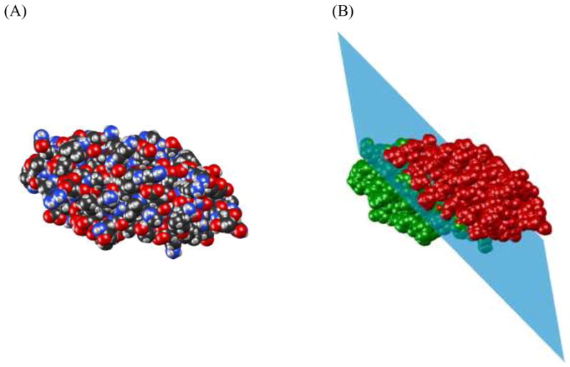
Illustration of the bisection of Cyanovirin-N (PDB code 2EZM). (A) Van der Waals surface of Cyanovirin-N. (B) Illustration of how the protein is split into two domains with approximately equal number of atoms by a plane. The first domain is colored green, the second domain is red.
Finally we applied our method to two protein-protein systems for which we have experimental RDC and CSP data: ubiquitin/UBA complex30 (PDB code 2JY6) and lysine-48-linked di-ubiquitin14 (PDB code 2BGF). These complexes allow us to present a “real world” practical application for PATIDOCK. We show that it is possible to quickly get a good solution for a complex using only the alignment tensor. In addition we show that combining our method with a more complicated energy function that accounts for additional factors such as van der Waals interactions and CSPs can yield an accurate solution in practice.
We implemented PATIDOCK in MATLAB 7.8.0 and performed all calculations and timing on a single core of 3.16 GHz Pentium Core 2 Duo E8500 processor with 3.25 GB of RAM, running Windows XP Service Pack 3. The set of [α,u] values for which we precompute F, η1, η2, and R was determined by the adaptive numerical integration of Equation (4) with an absolute error of 0.05 (using MATLAB’s quad function, see e.g.,31). The terminating condition for the Levenberg-Marquardt algorithm (MATLAB’s lsqnonlin function) was set to the step size less than 0.1Å. The 0.05 value was determined empirically based on the highest tolerance value which still gave docking solutions accurate to within 0.3Å for synthetic RDCs for all complexes in the COMPLEX and SINGLE datasets. Accuracy can be increased, at the expense of time, by changing the tolerance to the numerical integration routine. Note, however, that the improvement in accuracy is limited by the inherent inability of the barrier model to fully model the physical conditions.
Due to the four-fold ambiguity of the relative orientation of domain S2 with respect to S1 and the existence of multiple local minimizers (with regard to translation) for each orientation, we expect to have at least eight potential solutions. The solutions are ranked by the backbone RMSD between the experimental structure of the complex and the predicted one, where the atom positions in S2 are adjusted by R* and x* (recall that S1 is fixed in space). Only the results for the lowest-RMSD solution are shown in this paper. Since R* can be directly computed from the experimental RDC data independent of our model, we first focus our analysis on the minimizers that come from the correct orientation of the two domains. We then present the results for the complete docking method that also includes automatic alignment of the two domains, in addition to their positioning relative to each other.
Docking Using Ideal Synthetic Data
In order to demonstrate the feasibility of structural assembly of molecular complexes based solely on RDC data, we first applied PATIDOCK-t to synthetic data generated for proteins from the COMPLEX and SINGLE datasets.
To test our ability to find the correct minimizer under ideal conditions, for each complex we generated a synthetic alignment tensor Ãsyn using PATI prediction. From this and the three-dimensional structure of the complex we calculated RDCs for all amide NH bonds, which we call synthetic RDCs, assuming that there is no noise in experimental measurements. The synthetic RDCs along with the three-dimensional structures of the two domains comprise the input to our minimization algorithm. We will rate our results based on the “Δc”, the smallest distance between the original and all the predicted center of the second domain. The results for PATIDOCK-t, using Ãsyn as the “experimental” alignment tensor, are presented in Table 1 (columns “0 Hz”, “Time(s)”, and “#Sol.”) for the SINGLE dataset. The results for the COMPLEX dataset under ideal conditions (labeled “0 Hz” in Figure 2) are very similar (also see Supporting Information). These results clearly demonstrate that it is possible, under ideal conditions, to accurately and efficiently assemble molecular complexes based solely on RDC data.
Table 1.
The results of RDC-guided docking using PATIDOCK-t for the SINGLE dataset based on synthetic RDC data with added experimental noise.
| Protein | PDBa | 0 Hzb | 1 Hzb,c | 3 Hzb,c | Time(s)d | #Sol.e |
|---|---|---|---|---|---|---|
| B1 domain of protein G32 | 3gb1 | 0.07 [0.07] | 0.26 [0.97] | 0.67 [3.11] | 1.46 | 2 |
| B3 domain of protein G33 | 2oed | 0.09 [0.05] | 0.42 [1.02] | 1.31 [2.78] | 1.55 | 2 |
| Cyanovirin-N34 | 2ezm | 0.03 [0.02] | 0.31 [1.01] | 0.70 [2.90] | 2.81 | 3 |
| Gα interacting protein35 | 1cmz | 0.03 [0.02] | 0.35 [1.00] | 1.02 [2.94] | 2.23 | 2 |
| Ubiquitin36 | 1d3z | 0.02 [0.02] | 0.27 [0.97] | 0.66 [2.83] | 1.64 | 2 |
| Hen lysozyme37 | 1e8l | 0.05 [0.04] | 0.15 [1.00] | 0.49 [2.88] | 1.75 | 2 |
| Oxidized putidaredoxin38 | 1yjj | 0.06 [0.05] | 0.19 [1.00] | 0.71 [2.86] | 1.85 | 2 |
| Mean | 0.05 [0.04] | 0.28 [1.00] | 0.79 [2.90] | 1.90 | 2.14 | |
The RCSB Protein Data Bank code for protein coordinates. First model from the ensemble of NMR structures was used for all calculations.
Δc (in Å), the best distance between the original and the predicted centers of the second domain. The values in brackets represent the RMSD (in Hz) between the synthetic RDCs and the predicted RDCs at the solution. The column labels represent the size of the standard deviation of the normally distributed noise added to synthetic RDCs. “0 Hz” corresponds to no noise added to synthetic RDCs.
The values represent an average of twelve independent runs.
The average elapsed time (in seconds) for PATIDOCK-t based on all the runs for “0 Hz”, “1 Hz”, and “3 Hz”.
The number of possible solutions, all of which have a very similar predicted alignment tensor.
Figure 2.

PATIDOCK-t docking results for the 84 complexes in the COMPLEX dataset using synthetic RDC values with no noise (0 Hz, red circles) or in the presence of a Gaussian noise with the standard deviation of 1 Hz (green squares) or 3 Hz (blue diamonds) (see Supporting Table S1). (A) PATIDOCK-t docking results when all of the NH bond vectors are used in the computation of the alignment tensor. (B) PATIDOCK-t docking results when only 100 randomly selected NH bond vectors from the complex are used. Similar results were obtained when using only 50 randomly selected NH bond vectors (Supporting Table S1). The height constant h was adjusted for each complex to give a Da value of 20 Hz for Ãsyn, which corresponds to the average Da value of the SINGLE dataset, ubiquitin/UBA complex, and di-ubiquitin complex. In the case of noisy data, docking of each complex was performed six times, with individual RDC errors randomly selected from a normal distribution. All six results for each complex with RDC errors are plotted. For the purposes of visualization a few outliers for complexes 43 and 46 are not displayed. Bigger errors for some complexes reflect a much lesser sensitivity of the molecular shape (hence of the alignment tensor) of these specific complexes to translations of one domain relative to the other. (C-F) Van der Waals surface representation of the major outliers: (C-D) complex #43, PDB code 1I4D (mass 47 kDa, S1=chain D, S2=chains A and B); (E-F) complex #46, PDB code 1IBR (mass 77 kDa, S1=chain B, S2=chain A). The structures in (D) and (F) are rotated counterclockwise around the z-axis by 90°. The individual domains are colored green (S1) and red (S2), the convex hull of the complex is colored light blue.
Robustness of RDC-Guided Docking to Experimental Noise
In reality, RDC values always contain measurement errors, which are usually below 1 Hz. To assess the effect of such errors on the RDC-guided docking we added to the synthetic RDCs normally distributed noise with standard deviation of 1 Hz or 3 Hz. This allowed us to test whether it is possible to accurately dock a complex based solely on the alignment tensor in the presence of considerable (1 Hz) or extreme (3 Hz) noise in the data. Figure 2 shows errors in the docking solutions for the COMPLEX dataset in the presence or absence of random noise in the generated RDC values. Very similar results were obtained using synthetic RDC data (with noise) generated for the SINGLE dataset; see Table 1, columns “1 Hz” and “3 Hz”.
From these results (Figure 2 and Table 1) we conclude that PATIDOCK-t is able to find correct docking solutions for a wide variety of proteins even under heavy (3 Hz) experimental noise. These results validate the concept of molecular docking based exclusively on the alignment tensor.
PATIDOCK-t is also extremely fast, as it takes only seconds to dock two domains on a single PC. This speed makes it feasible to perform RDC-based docking at each iteration step of a more complicated flexible docking algorithm, for example by analyzing docking of multiple conformers at each minimization iteration. Another potential consequence of the speed is that it opens up the possibility of extending the docking algorithm to three or more molecules. Since we are able to accurately dock molecules given perfect prediction of the alignment tensor, the accuracy of the results in practice will depend on how well we can predict the alignment tensor in an experimental setting.
Docking using Experimental RDC Data
Having established the ability to accurately assemble molecular complexes using synthetic data, we next test our method on the alignment tensors derived from actual experimental data, in order to understand how errors in prediction of the alignment tensor affect the overall accuracy of docking. We use for this purpose the 7 proteins of the SINGLE dataset. The alignment tensor prediction and the limitations of the barrier model for these proteins were addressed in detail in our previous publication.8 Since the errors in the experimental RDC data for these proteins are about or smaller than 1 Hz, based on our results with synthetic data (Table 1) we expected to get a good solution provided that the barrier model is a good predictor of the alignment tensor. The results for PATIDOCK-t are shown in Table 2.
Table 2.
The results of RDC-guided docking using PATIDOCK-t for the SINGLE dataset based on experimental RDC data.
| Protein | PDBa | Δcb | RMSDRDCc | Time(s)d | #Sol.e |
|---|---|---|---|---|---|
| B1 domain of protein G | 3gb1 | 2.07 | 1.13 | 0.58 | 2 |
| B3 domain of protein G | 2oed | 4.15 | 1.32 | 0.61 | 2 |
| Cyanovirin-N | 2ezm | 5.01 | 4.00 | 0.75 | 2 |
| Gα interacting protein | 1cmz | 6.19 | 1.34 | 0.80 | 2 |
| Ubiquitin | 1d3z | 3.86 | 1.35 | 0.75 | 2 |
| Hen lysozyme | 1e8l | 3.42 | 7.24 | 0.94 | 2 |
| Oxidized putidaredoxin | 1yjj | 5.17 | 4.50 | 1.13 | 2 |
| Mean | 4.27 | 2.98 | 0.79 | 2.00 | |
The RCSB Protein Data Bank code for protein coordinates. First model from the ensemble of NMR structures was used for all calculations.
The distance (in Å) between the original and the predicted center of the second domain.
The RMSD (in Hz) between the experimental and the predicted RDC values at the best predicted minimizer.
The elapsed time (in seconds) required for docking.
The number of possible solutions, all of which have a very similar predicted alignment tensor.
Surprisingly, these solutions are worse than one would expect based just on the errors in the experimental data. Given that with synthetic RDC data these proteins were docked properly (see Table 1) this suggests that the alignment tensor predicted using a simple barrier model differs from the actual tensor, and this discrepancy could translate into an error (about 4.3Å) in the docking solution. In fact, as shown previously in Berlin et al.,8 the inaccuracy in alignment tensor prediction can be approximately separated into an error in the magnitude (scaling) of the tensor and an error in its orientation. On the positive side, however, the results in Table 2 show that by using only RDC data we are able to place the second domain on average within a radius of 4.3Å of its proper position.
Docking Using Experimental RDC Data: Combining Alignment and Translation
The docking efforts presented above focused on domain translation, while keeping interdomain orientation the same as in the original structure. We now combine our method for determining the correct translation with the method for aligning the two domains based on the orientations of the alignment tensor of the complex “reported” by each individual domain.9,11,13 This is the complete method, PATIDOCK, that takes two domains with arbitrary positions and orientations, and the associated experimental RDC values, and assembles their complex automatically with no human intervention at any step.
We first align the two domains by extracting (from the experimental RDC data for the complex) the alignment tensors “seen” by each domain and using Equation (1) to properly orient the second domain relative to the first one. Once the domains are oriented, we compute the experimental alignment tensor of the whole complex, Ã, from the RDC data and the combined bond vectors of the first domain and the newly oriented bond vectors of the second domain. This step helps average out experimental error and improve the accuracy of the resulting experimental alignment tensor by increasing the number of bond vectors used (generally resulting in improved orientational sampling22 and statistical averaging). We then use PATIDOCK to compute the proper translation between the now aligned domains. Due to the four-fold ambiguity in alignment we expect the number of solutions and the computation time to increase by a factor of four. The results for PATIDOCK with all potential solutions are shown in Table 3. Note that no domain alignment was performed in the PATIDOCK-t docking shown in Table 2, so the values in “Δc” column of that table are also “RMSD2” values as defined in Table 3.
Table 3.
The results of RDC-guided docking using PATIDOCK for the SINGLE dataset based on experimental RDC data.
| Protein | PDBa | RMSDb | RMSD2c | Δcd | RMSDRDCe | Time(s)f | #Sol.g |
|---|---|---|---|---|---|---|---|
| B1 domain of protein G | 3gb1 | 0.92 | 2.14 | 2.02 | 1.17 | 2.20 | 8 |
| B3 domain of protein G | 2oed | 1.68 | 4.30 | 4.28 | 1.20 | 2.08 | 8 |
| Cyanovirin-N | 2ezm | 1.92 | 5.02 | 5.02 | 3.99 | 2.56 | 10 |
| Gα interacting protein | 1cmz | 2.72 | 7.04 | 6.75 | 1.40 | 2.63 | 8 |
| Ubiquitin | 1d3z | 1.79 | 3.77 | 3.76 | 1.29 | 2.66 | 9 |
| Hen lysozyme | 1e8l | 1.60 | 3.29 | 3.29 | 7.20 | 3.19 | 8 |
| Oxidized putidaredoxin | 1yjj | 2.51 | 5.40 | 5.32 | 4.53 | 2.94 | 9 |
| Mean | 1.88 | 4.42 | 4.35 | 2.97 | 2.61 | 8.43 | |
The RCSB Protein Data Bank code for protein coordinates. First model from the ensemble of NMR structures was used for all calculations.
The backbone RMSD (in Å) between the original complex structure and the predicted complex. The structures are optimally rotated and centered using the center of mass.39
The backbone RMSD (in Å) between the coordinates of atoms of the second domain for the original and the predicted complex.
The distance (in Å) between the original and the predicted center of the second domain. The center is computed as the average of the positions of all the atoms in the domain.
The RMSD (in Hz) between the experimental and the predicted RDC values at the best predicted minimizer.
The elapsed time (in seconds) required for docking of all four orientations.
The number of possible solutions, all of which have a very similar predicted alignment tensor.
The error in the relative position of the second domain (see Δc in Table 3) changed only slightly (an increase by 0.08Å on average) compared to the PATIDOCK-t method. Combined with the small increase (0.15Å on average) in RMSD2 values from the fixed-orientation assembly in Table 2 (values in the “Δc” column) to the align-and-translate assembly in Table 3, these results indicate that alignment of domains by using experimental RDC values is a robust and accurate technique and is not a significant contributor of error to structure assembly. As expected, there is a four-fold increase in the number of possible solutions and the running time, but the combined algorithm still completes in less than four seconds.
Application to a Real System: Ubiquitin/UBA Complex
We now test our method on a protein complex for which experimental RDC and CSP data are available: the complex of human ubiquitin (Ub) with the UBA domain of ubiquilin-130 (PDB code 2JY6). Using the experimental CSP data we defined as CSP-active residues L8, T9, G10, K48, E51, R54, Q62, H68, L71, and L73 in Ub, and M557, G558, L560, I570, A571, N577, E581, R582, L584 in UBA. See Figure 3 for the mapping of the CSP-active residues onto the Ub/UBA complex. In this section we will only use the RDC data, while the CSP data will be included in a later section.
Figure 3.
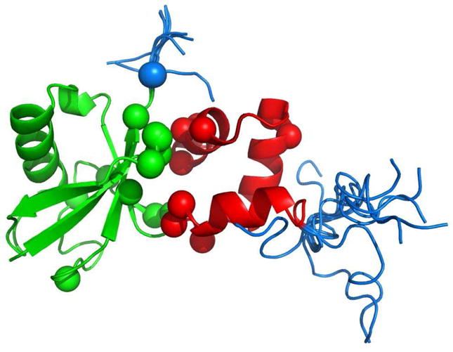
A cartoon representation of the ensemble of 100 possible models for the Ub/UBA complex (Structure 2jy6-I). Ub is colored green, UBA is in red, the flexible tails are colored blue, and the CSP-active residues are represented by spheres around their Cα atoms.
A potential complication for the rigid-body docking approach arises in the case of the Ub/UBA complex from the fact that both proteins have extended unstructured and highly flexible tails. In fact, residues 73–76 in Ub and 536–544 in the UBA construct used in the experimental study experience large-amplitude motions30 on a ps-ns time scale, which is many orders of magnitude faster than the time scale (~100 ms) of a NMR experiment. These motions are also present in the Ub/UBA complex, reflecting the fact that the tails do not participate in the binding.30 Naturally, such tails present a significant challenge for shape-sensitive computations like those in the current study, because no single structure can represent the ensemble/motion-averaged molecular shape relevant for a particular experiment. This raises important questions that have not been addressed in the literature so far: could flexible tails simply be neglected (clipped off) in such calculations or should they be represented by a structural ensemble, and how large does the latter need to be? In order to address these questions, we performed docking for both the structural ensembles and the clipped (tailless) structures. Because the RDC data were measured in the PEG/hexanol medium,12 the actual inter-barrier distance was unknown and had to be estimated. We set h = 400Å, a value that gives the correct scaling between the predicted and experimentally determined alignment tensor at the known solution.
To sample various orientations of the tails (not present in the original PDB structure of the complex), we extracted 10 representative orientations of Ub’s C-terminus from the NMR ensemble of Ub monomer (PDB code 1D3Z36) and 10 possible orientations of the N-terminus of the UBA domain from its NMR ensemble in the monomeric state (PDB code 2JY530). These conformations of the tails were superimposed onto the corresponding domains in the complex structure (2JY6), thus creating an ensemble of 100 possible models for the Ub/UBA complex (shown in Figure 3). We refer to this Ub/UBA complex as Structure 2jy6-I. From the 100 models of Structure 2jy6-I we were able to estimate the variance in the docking solutions that the two tails introduce. The results are presented in Table 4.
Table 4.
The results of docking the Ubiquitin/UBA complex using PATIDOCK-t and PATIDOCK.
| Structurea | Methodb | RMSDc | RMSD2d | Δce | RMSDRDCf | Time(s) | #Sol.g |
|---|---|---|---|---|---|---|---|
| 2jy6-I | PATIDOCK-t | 3.39h (1.06)h | 8.75h (1.96)i | 8.75h (1.96)i | 4.31h (1.15)i | 0.81h (0.12)i | 2.01h |
| 2jy6-I | PATIDOCK | 3.46h (1.09)i | 8.75h (2.03)i | 8.72h (2.03)i | 4.25h (1.16)i | 2.30h (0.30)i | 8.23h |
| 2jy6-II | PATIDOCK-t | 1.29 | 4.23 | 4.23 | 4.14 | 0.70 | 2 |
| 2jy6-II | PATIDOCK | 1.23 | 3.74 | 3.70 | 4.17 | 2.17 | 8 |
2jy6-I is the ensemble of 100 structures representing various conformations of Ub and UBA tails (see text), whereas in 2jy6-II the tails were clipped off.
The method that was used to dock the complex.
The backbone RMSD (in Å) between the original complex structure and the predicted complex. The structures are optimally rotated and centered using the center of mass.39
The backbone RMSD (in Å) between the coordinates of atoms of the second domain for the original and predicted complex.
The distance (in Å) between the original and the predicted center of the second domain. The center is computed as the average of the positions of all the atoms in the domain.
The RMSD (in Hz) between the experimental and the predicted RDC values at the best predicted minimizer.
The number of possible solutions, all of which have a very similar overall alignment tensor.
Values are the means of the individual values for the best solution of each of the 100 models.
Values in the parentheses are the standard deviations of the individual values for the best solution of each of the 100 models.
Because averaging by fast reorientations of the tails is expected to diminish the tails’ effect on the alignment tensor, we clipped off the two tails from the structures of the corresponding proteins and then docked the two tailless molecules using PATIDOCK-t and PATIDOCK. We refer to the tailless Ub/UBA complex as Structure 2jy6-II; the results are presented in Table 4. Figure 4 shows the isosurface plot of the energy function χ2 for the tailless Ub/UBA complex and the visualization of the two solutions from PATIDOCK-t. The isosurface plot clearly demonstrates that there are two distinct minima in the energy function, both of which were found by our program. As can be seen from Figure 4C and Figure 4D, the reason for the two minima is that both solutions have very similar convex hulls due to the geometric symmetry inherent in the problem.
Figure 4.

The results of RDC-guided docking for the tailless Ub/UBA complex (2jy6-II) using PATIDOCK-t. Shown are (A–B) isosurface plots of the χ2(x) function and (C-D) the associated van der Waals surfaces (wrapped by their convex hulls) of the two solutions corresponding to the two local minima of χ2(x). The isosurfaces correspond to (A) minxχ2(x) + 0.1σ and (B) minxχ2(x) + 0.6σ, for all x inside the grid, where σ is the standard deviation of the values of χ2 in the grid. The isosurface data were collected on a 100 × 100 × 100 Å grid around 0. (C) The best (closest) solution with the UBA domain positioned to the right of Ub, with χ2 = 2.01 × 10⁻⁷ at the solution. (D) The incorrect solution where the UBA domain is to the left of Ub, with χ2 = 1.24 ×10⁻⁷ at the solution. In these van der Waals surface plots Ub is colored green and UBA is red. Both solutions have a very similar convex hull, hence similar predicted alignment tensor. The camera angle relative to Ub’s orientation is the same in both figures. Note that the best solution has a higher χ2 value.
As evident from Table 4, the conformation(s) of the tail can have a profound effect on the results of docking. The solution varies on average by 2Å over all the possible combinations of tail orientations, whereas removing the tails improves the results significantly. This suggests that a potential solution for dealing with flexible tails in RDC-guided docking is to clip them off rather than use a specific conformation or try to deduce the “averaged” conformation of the tail. Without the tails, using PATIDOCK, we get the Δc and RMSD2 of about 3.7Å, which are smaller than the expected average position error of about 4.4Å (see Table 2 and Table 3).
Application to a Real Dual-Domain System: Lys48-linked di-Ubiquitin
Finally, we tested our method on a dual-domain system for which both experimental RDC and CSP data are available: the Lys48-linked di-Ubiquitin12–14 (PDB code 2BGF). Using the experimental CSP data we define hydrophobic-patch residues L8, I44, and L70 on both domains to be CSP-active. See Figure 5 for the mapping of the CSP-active residues onto the di-Ubiquitin (Ub2) structure. The CSP data will be used in a later section. Because the RDC data were measured in the PEG/hexanol medium,12 the actual inter-barrier distance was unknown and had to be estimated. We set h = 550Å, a value that gives the correct scaling between the predicted and experimentally determined alignment tensor at the known solution.
Figure 5.
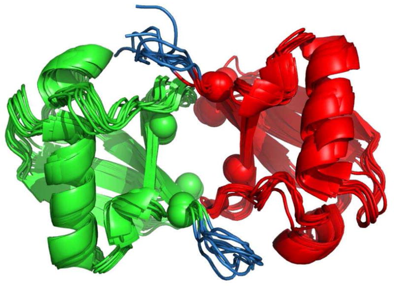
A cartoon representation of the ensemble of 10 models for the di-Ubiquitin complex (Structure 2bgf-I). Proximal domain is colored green, distal domain is in red, the flexible tails are colored blue, and the CSP-active residues are represented by spheres around their Cα atoms.
As in the case of the Ub/UBA complex, a potential complication for the rigid-body docking approach arises from the unstructured and highly flexible C-terminal tails comprising residues 73–76 of each domain,13 though the tail in Ub is much shorter than that of UBA. We therefore performed a similar analysis to that in the previous section. However, instead of superimposing the tails onto the Ub2 complex, we simply took the ensemble of the 10 models from the Ub2 structure 2BGF (shown in Figure 5). We refer to this ensemble as Structure 2bgf-I. Similarly, we created Structure 2bgf-II by taking the first model in 2BGF and clipping off residues 73–76 of both domains. The results for the ensemble and the clipped (tailless) structures are presented in Table 5.
Table 5.
The results of docking Lys48-linked di-Ubiquitin using PATIDOCK-t and PATIDOCK.
| Structurea | Methodb | RMSDc | RMSD2d | Δce | RMSDRDCf | Time(s) | #Sol.g |
|---|---|---|---|---|---|---|---|
| 2bgf-I | PATIDOCK-t | 1.34h (0.38)i | 3.97h (1.22)i | 3.97h (1.22)i | 3.59h (0.38)i | 0.88h (0.08)i | 2.20h |
| 2bgf-I | PATIDOCK | 1.45h (0.28)i | 4.27h (0.65)i | 4.13h (0.64)i | 3.44h (0.33)i | 2.81h (0.29)i | 8.10h |
| 2bgf-II | PATIDOCK-t | 1.09 | 3.71 | 3.71 | 3.47 | 1.06 | 2 |
| 2bgf-II | PATIDOCK | 1.14 | 3.67 | 3.61 | 3.49 | 2.86 | 8 |
2bgf-I is the ensemble of 10 structures representing various conformations of the C-terminal tails of both Ub molecules (see text), whereas in 2bgf-II the tails were clipped off.
The method that was used to dock the complex.
The backbone RMSD (in Å) between the original complex structure and the predicted complex. The structures are optimally rotated and centered using the center of mass.39
The backbone RMSD (in Å) between the coordinates of atoms of the second domain for the original and the predicted complex.
The distance (in Å) between the original and the predicted center of the second domain. The center is computed as the average of the positions of all the atoms in the domain.
The RMSD (in Hz) between the experimental and the predicted RDC values at the best predicted minimizer.
The number of possible solutions, all of which have a very similar overall alignment tensor.
Values are the means of the individual values for the best solution of each of the 100 models.
Values in the parentheses are the standard deviations of the individual values for the best solution of each of the 100 models.
As above, the conformation of the tail has noticeable effect on the results of docking, although significantly less than in the Ub/UBA complex. The solution varies on average by 1Å among all the possible tails’ conformations, and removing the tails improves the results slightly. These results further support the conclusion that the potential solution for dealing with flexible tails in RDC-guided docking is to clip off the tails. Without the tails, using PATIDOCK, we get the errors in positioning of the second domain of Δc = 3.6Å and RMSD2 = 3.7Å, which are smaller than the expected average value of about 4.4Å (see above).
Docking Using Experimental RDC Data Combined with Ambiguous Interface-Related Restraints
The results in previous sections using real experimental data give a good hint at the errors that one can expect when using the barrier model as the alignment tensor predictor. Thus, we expect that in practice the error in domain positioning using PATIDOCK would be less than 5Å. The fact that the results are a relatively short distance from the actual solution demonstrates that the alignment-tensor-based χ2 is a useful constraint.
We now seek to improve upon the previous results by combining CSP-like constraints along with the alignment tensor constraints by minimizing (see Equation (15)). The combination of constraints should lead to a better and more reliable overall solution. The results of applying PATIDOCK+ to the SINGLE dataset, Ub/UBA, and Ub2 are presented in Table 6. Note that we are now able to select the correct structure out of all possible solutions by picking the one with the lowest value. The cartoon representations of the solutions for the two protein-protein systems are presented in Figure 6.
Table 6.
The results for PATIDOCK+ using a combination of CSP-like and alignment tensor constraints.
| Protein | Structurea | RMSDb | RMSD2c | Δcd | RMSDRDCe | #Sol.f |
|---|---|---|---|---|---|---|
| B1 domain of protein G | 3gb1 | 0.92 | 2.01 | 1.89 | 1.63 | 1 |
| B3 domain of protein G | 2oed | 1.17 | 3.23 | 3.22 | 1.66 | 1 |
| Cyanovirin-N | 2ezm | 1.44 | 3.93 | 3.93 | 3.98 | 1 |
| Gα interacting protein | 1cmz | 1.15 | 3.53 | 3.10 | 2.67 | 1 |
| Ubiquitin | 1d3z | 1.00 | 2.46 | 2.46 | 2.27 | 1 |
| Hen lysozyme | 1e8l | 0.90 | 1.94 | 1.94 | 7.36 | 1 |
| Oxidized putidaredoxin | 1yjj | 1.34 | 3.15 | 3.03 | 4.40 | 1 |
| Ubiquitin/UBA | 2jy6-II | 0.57 | 1.37 | 1.28 | 4.91 | 1 |
| di-Ubiquitin | 2bgf-II | 0.78 | 1.73 | 1.59 | 4.28 | 1 |
| Mean | 1.03 | 2.60 | 2.49 | 3.69 | 1.00 | |
See previous tables and Results section for structure references.
The backbone RMSD (in Å) between the original complex structure and the predicted complex. The structures are optimally rotated and centered using the center of mass.39
The backbone RMSD (in Å) between the coordinates of atoms of the second domain for the original and predicted complex.
The distance (in Å) between the original and the predicted center of the second domain. The center is computed as the average of the positions of all the atoms in the domain.
The RMSD (in Hz) between the experimental and the predicted RDC values at the best predicted minimizer.
The number of possible solutions, all of which have a very similar .
Figure 6.

A cartoon representation of the actual structure (green) vs. the docked structure (red) for the (A) Ub/UBA complex and (B) Ub2 molecule based on minimization of . Only the adjusted domain (S2, right) is shown for the docked structures, the other domain (S1, left) superimposes exactly with the corresponding domain in the actual structure.
As evident from Table 6, the addition of ambiguous, CSP-like restraints significantly improved the solution for all proteins, compared to the results in Table 3, Table 4, and Table 5. The docked solutions for the two “real” complexes (Ub/UBA and Ub2) based entirely on experimental RDC and CSP data have both Δc and RMSD2 below 2Å. This indicates that combining RDCs with other experimental intermolecular constraints in a real situation could be a powerful method for quickly yielding good docking solutions. The additional benefit of using CSP-like restraints is that we now are able to correctly identify the best solution from the eight or more possible symmetry-related solutions based just on the values.
Docking Using Unbound Structures
In some docking applications structures of the individual components in the bound state might not be known in advance, but are to be determined in the process of docking, for example, using the “unbound” structures of the domains as the starting point. We therefore examine how accurately our method positions two domains relative to each other given only the RDC data for the bound complex and the unbound structures of the two domains, i.e. how robust our method is with regard to structural rearrangements in the individual components resulting from binding interactions. Generally, we anticipate several sources of inaccuracy in the resulting RDC-guided complexes when using unbound structures of the individual components. These include (i) inaccuracy in the derived experimental alignment tensor(s), due to a different orientation of the RDC-active bond vectors, and (ii) a different 3D shape of each component (and their complex), which would affect the predicted alignment tensor. Perturbations in intermolecular contacts at the interface, reflecting different orientations of the side chains, could also affect the accuracy of docking, when contact-based restraints are included (see above).
Here we take advantage of the availability of both bound and unbound structures for the 84 proteins of the COMPLEX dataset.28 The synthetic RDCs generated for each bound complex as described above (zero noise) were used as input “experimental” RDC data for the same complex, but applied to unbound structures of each domain. Using the NH bond vectors of the unbound structures and the synthetic RDCs, we computed the alignment tensors “reported” by each of the domains, and used the same docking procedure as above (PATIDOCK-t or PATIDOCK) to assemble the corresponding complex of the unbound individual components.
We compare the resulting structures (docked “unbound” complexes) with the corresponding complexes of the bound structures in Figure 7. The results are presented in terms of RMSDs for all backbone atoms. These numbers should be compared to the “Base” RMSD level (red bars in Figure 7) that reflects the structural differences between the unbound and bound structures of the individual domains, calculated by superimposing the unbound structure of each domain onto the bound structure in the complex and computing the overall (backbone) RMSD. The results show that structural/dynamic rearrangements in the individual components upon complex formation do not dramatically affect the relative domain positioning in the resulting RDC-guided structures. The average error in the position of the second domain (Δc) for PATIDOCK-t and PATIDOCK was about 5Å.
Figure 7.

The results of PATIDOCK-t (green bars) and PATIDOCK (blue bars) assembly of complexes of “unbound” structures of the proteins from the COMPLEX dataset, using synthetically generated alignment tensors from the corresponding “bound” complexes as the target experimental alignment tensor to guide the docking. Shown are backbone RMSDs between the resulting (unbound) complex and the original (bound) complex. “Base” RMSDs (red bars) reflect the structural differences between the unbound and bound structures of the individual domains, calculated by superimposing the unbound structure of each domain onto the bound structure in the complex and computing the overall RMSD. Missing bars correspond to those few complexes where we were unable to properly match the atoms between the bound and the unbound coordinate sets.
Finally, we examine the performance of RDC-guided docking of unbound structures when using real experimental RDC data. We use the unbound tailless structures of ubiquitin (PDB code 1D3Z) and UBA (PDB code 2JY5) to assemble the Ub/UBA and Ub2 complexes using experimental RDCs for their bound complex. The results, shown in Table 7, are similar to the COMPLEX dataset using synthetic data, shown in Figure 7.
Table 7.
The results of docking the unbound Ubiquitin/UBA and Lys48-linked di-Ubiquitin complexes using PATIDOCK-t and PATIDOCK.
| Complexa | Methodb | Base RMSDc | RMSDd | RMSD2e | Δcf | RMSDRDCg | #Sol.h |
|---|---|---|---|---|---|---|---|
| Ubiquitin/UBA | PATIDOCK-t | 0.97 | 1.50 | 3.93 | 3.84 | 6.55 | 2 |
| Ubiquitin/UBA | PATIDOCK | 0.97 | 2.67 | 6.24 | 4.47 | 5.87 | 8 |
| di-Ubiquitin | PATIDOCK-t | 0.94 | 1.52 | 3.61 | 3.48 | 2.75 | 2 |
| di-Ubiquitin | PATIDOCK | 0.94 | 4.17 | 9.43 | 6.89 | 2.62 | 8 |
For this docking we used unbound tailless structures of ubiquitin (PDB code 1D3Z) and UBA (PDB code 2JY5). The resulting structures of the ubiquitin/UBA and di-ubiquitin complexes were compared with the corresponding tailless (bound) complexes, 2JY6-II and 2BGF-II, respectively.
The method that was used to dock the complex.
The structural differences (in Å) between the unbound and bound structures of the individual domains, calculated by superimposing the unbound structure of each domain onto the bound structure in the complex and computing the overall RMSD.
The backbone RMSD (in Å) between the original complex structure and the predicted complex. The structures are optimally rotated and centered using the center of mass.39
The backbone RMSD (in Å) between the coordinates of atoms of the second domain for the original and the predicted complex.
The distance (in Å) between the original and the predicted center of the second domain. The center is computed as the average of the positions of all the atoms in the domain.
The RMSD (in Hz) between the experimental and the predicted RDC values at the best predicted minimizer.
The number of possible solutions, all of which have a very similar overall alignment tensor.
These results indicate that the RDC-guided docking is relatively robust with respect to structural rearrangements induced by complex formation. This is likely due to statistical averaging during the RDC to alignment tensor conversion. Moreover, this finding also suggests that the unbound structures of the individual components could be used as a crude, initial approximation for the complex assembly, to be followed by more rigorous docking steps that allow structural flexibility and adaptation necessary for final adjustment of the individual components in the complex.
Conclusions
In this paper we demonstrated that it is fundamentally possible to assemble a protein-protein complex based solely on experimental RDC data and the prediction of the alignment tensor from three-dimensional structures, provided that the structures of the individual components are available. To achieve this, we reduced the multitude of experimental RDCs to a single alignment tensor consisting of five independent parameters, and then used the latter to guide positioning and orientation of one domain relative to the other. During the docking process, the alignment tensor acts as a “mechanical” constraint applied to the interdomain vector and forcing the individual components to adopt a particular position within the molecule such that the molecular shape of the resulting complex matches that of the real one (as far as the alignment tensor is concerned). The ability to assemble a molecular complex using RDCs is remarkable, because it shows that despite the purely angular nature of residual dipolar couplings, they can be translated into distance/translational constraints. This is due to RDC’s sensitivity to molecular shape and reflects the fact that it is the shape of the molecule that causes its steric alignment.
The PATIDOCK method is robust with respect to large experimental errors in RDC data, provided there are a sufficient number of experimental RDCs. This is not surprising since the alignment tensor “averages” the information contained in the RDCs. By extension, the inherent averaging of RDCs in the alignment tensor makes PATIDOCK also somewhat robust against local structural rearrangements/dynamics associated with complex formation. When applied to real experimental data, PATIDOCK gives on average a less than 5Å error in the relative positioning of the molecules. We demonstrated that the resulting structure could be further refined by including other available experimental data (PATIDOCK+). Moreover, the presence of extended unstructured/flexible parts (e.g. tails) in a molecule can potentially affect the solution by more than 2Å, depending on which structure/conformation of such parts is chosen. We propose removal of the flexible tails as a potential solution to this problem.
The PATIDOCK methods are extremely fast, and therefore we do not foresee a need for a faster, but less accurate, method for prediction of the alignment tensor than PATI. Potential improvements in the prediction of the alignment tensor will most likely involve (i) representing individual molecular components as structural ensembles rather than single structures and (ii) using a weight function inside the integrals in Equation (4), to account for possible non-steric interactions with the aligning medium. For example, such a function could weigh η differently, or introduce charge potentials in case of non-neutral alignment media (see e.g.,23). We foresee such an addition as being easily adapted into our docking method.
It is worth mentioning that accutate characterization of protein-protein complexes should account for contributions to the experimental RDC data from free components in fast exchange with the complex (see e.g.40). This is particularly true for weak macromolecular interactions. Application to such systems would require modification of the target function in equation (3) to include the contributions to experimental data from the free form of the interacting partners.
The PATIDOCK approach presented in this paper can potentially be used in several ways. First, it provides a quick rigid-body docking method whose solutions can be utilized to significantly limit the search space of a more complicated flexible-docking algorithm. The robustness of the approach with respect to structural rearrangements suggests that the RDC-guided docking could be used early on in the process of molecular complex assembly, e.g., starting with the unbound structures of the individual components, and subsequently refining them as the computation progresses. Second, our energy functions can be included as an additional term into a more general energy function that accounts for all other structure-related constraints such as distance and torsional angle restraints, hydrogen bonding, electrostatic and van der Waals potentials, etc. Moreover, the computational efficiency of the PATIDOCK method makes it feasible to perform RDC-based docking at each iteration step of a more complicated flexible-docking algorithm, for example by analyzing docking of multiple conformers at each minimization iteration. The molecular-shape-based RDC-guided docking can be incorporated into existing structure determination/refinement protocols (e.g. HADDOCK,25 XPLOR-NIH41). This would allow us to account for side chain and backbone flexiblity at the inerface and integrate with all other available experimental data. A recent XPLOR-NIH implementation42 of the diffusion-tensor-guided docking method20 serves as an example. Third, PATIDOCK can be used as the main method for driving molecular docking in a situation where there is a lack of unambiguous intermolecular structural information, like NOEs. This last application will become more practical as methods for prediction of the alignment tensor improve. Fourth, the energy function designed here could potentially also be used to evaluate and refine protein structures, including those for single-domain proteins, based on how well the 3D shape of the molecule agrees with experimental RDC data.
The fact that our docking method is extremely fast for two-domain complexes opens up the possibility of extending the PATIDOCK approach to three or more domains. Even though each additional domain gives rise to an exponential increase in complexity and time, it is still possible to quickly evaluate our energy function for a multitude of domains.
Supplementary Material
Acknowledgments
This work was supported by NIH grant GM065334 to D.F. The PATIDOCK program is available from the authors upon request.
Footnotes
Supporting Information Available
Formulae for F, a table with the results of docking for the COMPLEX dataset, and a table containing values of the energy functions at the known solutions. This material is available free of charge via the Internet at http://pubs.acs.org.
References
- 1.Tolman J, Flanagan J, Kennedy M, Prestegard J. Proceedings of the National Academy of Sciences of the United States of America. 1995;92:9279–9283. doi: 10.1073/pnas.92.20.9279. [DOI] [PMC free article] [PubMed] [Google Scholar]
- 2.Tjandra N, Bax A. Science. 1997;278:1111–1114. doi: 10.1126/science.278.5340.1111. [DOI] [PubMed] [Google Scholar]
- 3.Bax A. Protein Science. 2003;12:1–16. doi: 10.1110/ps.0233303. [DOI] [PMC free article] [PubMed] [Google Scholar]
- 4.Zweckstetter M, Bax A. Journal of the American Chemical Society. 2000;122:3791–3792. [Google Scholar]
- 5.Fernandes MX, Bernado P, Pons M, Garcia de la Torre J. Journal of the American Chemical Society. 2001;123:12037–12047. doi: 10.1021/ja011361x. [DOI] [PubMed] [Google Scholar]
- 6.Almond A, Axelsen J. Journal of the American Chemical Society. 2002;124:9986–9987. doi: 10.1021/ja026876i. [DOI] [PubMed] [Google Scholar]
- 7.Azurmendi HF, Bush CA. Carbohydrate Research. 2002;337:905–915. doi: 10.1016/s0008-6215(02)00070-8. [DOI] [PubMed] [Google Scholar]
- 8.Berlin K, O’Leary DP, Fushman D. Journal of Magnetic Resonance. 2009;201:25–33. doi: 10.1016/j.jmr.2009.07.028. [DOI] [PMC free article] [PubMed] [Google Scholar]
- 9.Fischer M, Losonczi J, Weaver J, Prestegard J. Biochemistry. 1999;38:9013–9022. doi: 10.1021/bi9905213. [DOI] [PubMed] [Google Scholar]
- 10.Skrynnikov N, Goto N, Yang D, Choy W, Tolman J, Mueller G, Kay L. Journal of Molecular Biology. 2000;295:1265–1273. doi: 10.1006/jmbi.1999.3430. [DOI] [PubMed] [Google Scholar]
- 11.Dosset P, Hus J, Marion D, Blackledge M. Journal of Biomolecular NMR. 2001;20:223–231. doi: 10.1023/a:1011206132740. [DOI] [PubMed] [Google Scholar]
- 12.Varadan R, Walker O, Pickart C, Fushman D. Journal of Molecular Biology. 2002;324:637–647. doi: 10.1016/s0022-2836(02)01198-1. [DOI] [PubMed] [Google Scholar]
- 13.Fushman D, Varadan R, Assfalg M, Walker O. Progress in Nuclear Magnetic Resonance Spectroscopy. 2004;44:189–214. [Google Scholar]
- 14.van Dijk A, Fushman D, Bonvin A. Proteins: Structure, Function, and Bioinformatics. 2005;60:367–381. doi: 10.1002/prot.20476. [DOI] [PubMed] [Google Scholar]
- 15.Clore GM. Proceedings of the National Academy of Sciences of the United States of America. 2000;97:9021–9025. doi: 10.1073/pnas.97.16.9021. [DOI] [PMC free article] [PubMed] [Google Scholar]
- 16.Clore GM, Schwieters CD. Journal of the American Chemical Society. 2003;125:2902–2912. doi: 10.1021/ja028893d. [DOI] [PubMed] [Google Scholar]
- 17.Blackledge M. Progress in Nuclear Magnetic Resonance Spectroscopy. 2005;46:23–61. doi: 10.1016/j.pnmrs.2017.06.001. [DOI] [PubMed] [Google Scholar]
- 18.Hu W, Wang L. Annual Reports of NMR Spectroscopy. 2006;58:232. [Google Scholar]
- 19.de Alba E, Baber JL, Tjandra N. Journal of the American Chemical Society. 1999;121:4282–4283. [Google Scholar]
- 20.Ryabov Y, Fushman D. Journal of the American Chemical Society. 2007;129:7894–7902. doi: 10.1021/ja071185d. [DOI] [PMC free article] [PubMed] [Google Scholar]
- 21.Losonczi JA, Andrec M, Fischer MWF, Prestegard JH. Journal of Magnetic Resonance. 1999;138:334–342. doi: 10.1006/jmre.1999.1754. [DOI] [PubMed] [Google Scholar]
- 22.Fushman D, Ghose R, Cowburn D. Journal of the American Chemical Society. 2000;122:10640–10649. [Google Scholar]
- 23.Zweckstetter M. Nature Protocols. 2008;3:679–690. doi: 10.1038/nprot.2008.36. [DOI] [PubMed] [Google Scholar]
- 24.Marquardt D. Journal of the Society for Industrial and Applied Mathematics. 1963;11:431–441. [Google Scholar]
- 25.Dominguez C, Boelens R, Bonvin A. Journal of the American Chemical Society. 2003;125:1731–1737. doi: 10.1021/ja026939x. [DOI] [PubMed] [Google Scholar]
- 26.de Vries S, van Dijk A, Krzeminski M, van Dijk M, Thureau A, Hsu V, Wassenaar T, Bonvin A. Proteins: Structure, Function, and Bioinformatics. 2007;69:726–733. doi: 10.1002/prot.21723. [DOI] [PubMed] [Google Scholar]
- 27.Lawler E, Wood D. Operations Research. 1966;14:699–719. [Google Scholar]
- 28.Mintseris J, Wiehe K, Pierce B, Anderson R, Chen R, Janin J, Weng Z. Proteins. 2005;60:214–216. doi: 10.1002/prot.20560. [DOI] [PubMed] [Google Scholar]
- 29.Ulrich E, et al. Nucleic Acids Research. 2008;36:D402–D408. doi: 10.1093/nar/gkm957. [DOI] [PMC free article] [PubMed] [Google Scholar]
- 30.Zhang D, Raasi S, Fushman D. Journal of Molecular Biology. 2008;377:162–180. doi: 10.1016/j.jmb.2007.12.029. [DOI] [PMC free article] [PubMed] [Google Scholar]
- 31.Van Loan CF. Introduction to Scientific Computing: A Matrix-Vector Approach Using MAT-LAB. Prentice-Hall, Inc; Upper Saddle River, NJ, USA: 1997. [Google Scholar]
- 32.Kuszewski J, Gronenborn AM, Clore GM. Journal of the American Chemical Society. 1999;121:2337–2338. [Google Scholar]
- 33.Ulmer TS, Ramirez BE, Delaglio F, Bax A. Journal of the American Chemical Society. 2003;125:9179–9191. doi: 10.1021/ja0350684. [DOI] [PubMed] [Google Scholar]
- 34.Bewley C, Gustafson K, Boyd M, Covell D, Bax A, Clore G, Gronenborn A. Nature Structural Biology. 1998;5:571–578. doi: 10.1038/828. [DOI] [PubMed] [Google Scholar]
- 35.de Alba E, De Vries L, Farquhar M, Tjandra N. Journal of Molecular Biology. 1999;291:927–939. doi: 10.1006/jmbi.1999.2989. [DOI] [PubMed] [Google Scholar]
- 36.Cornilescu G, Marquardt JL, Ottiger M, Bax A. Journal of the American Chemical Society. 1998;120:6836–6837. [Google Scholar]
- 37.Schwalbe H, Grimshaw S, Spencer A, Buck M, Boyd J, Dobson C, Redfield C, Smith L. Protein Science. 2001;10:677–688. doi: 10.1110/ps.43301. [DOI] [PMC free article] [PubMed] [Google Scholar]
- 38.Jain NU, Tjioe E, Savidor A, Boulie J. Biochemistry. 2005;44:9067–9078. doi: 10.1021/bi050152c. [DOI] [PubMed] [Google Scholar]
- 39.McLachlan A. Journal of Molecular Biology. 1979;128:49–79. doi: 10.1016/0022-2836(79)90308-5. [DOI] [PubMed] [Google Scholar]
- 40.Ortega-Roldan JL, Jensen MR, Brutscher B, Azuaga AI, Blackledge M, van Nuland NAJ. Nucleic Acids Research. 2009;37:e70–e70. doi: 10.1093/nar/gkp211. [DOI] [PMC free article] [PubMed] [Google Scholar]
- 41.Schwieters C, Kuszewski J, Tjandra N, Marius Clore G. Journal of Magnetic Resonance. 2003;160:65–73. doi: 10.1016/s1090-7807(02)00014-9. [DOI] [PubMed] [Google Scholar]
- 42.Ryabov Y, Suh JY, Grishaev A, Clore GM, Schwieters CD. Journal of the American Chemical Society. 2009;131:9522–9531. doi: 10.1021/ja902336c. [DOI] [PMC free article] [PubMed] [Google Scholar]
Associated Data
This section collects any data citations, data availability statements, or supplementary materials included in this article.