Dynamic Metabolic Flux Analysis Demonstrated on Cultures Where the Limiting Substrate Is Changed from Carbon to Nitrogen and Vice Versa

Abstract

The main requirement for metabolic flux analysis (MFA) is that the cells are in a pseudo-steady state, that there is no accumulation or depletion of intracellular metabolites. In the past, the applications of MFA were limited to the analysis of continuous cultures. This contribution introduces the concept of dynamic MFA and extends MFA so that it is applicable to transient cultures. Time series of concentration measurements are transformed into flux values. This transformation involves differentiation, which typically increases the noisiness of the data. Therefore, a noise-reducing step is needed. In this work, polynomial smoothing was used. As a test case, dynamic MFA is applied on Escherichia coli cultivations shifting from carbon limitation to nitrogen limitation and vice versa. After switching the limiting substrate from N to C, a lag phase was observed accompanied with an increase in maintenance energy requirement. This lag phase did not occur in the C- to N-limitation case.

1. Introduction

Material balances of reactors describe how certain compounds go in the reactor and are transformed into other compounds. Metabolic models consider the cell as the reactor and, additionally to the exchange rates, also include information on the different steps (reactions) on how the input compounds are transformed to the output compounds. This should allow to gain insight in the internal cellular fluxes. Typically the number of equations (material balances of the different compounds) obtained is less than the number of unknowns (exchange rates and reaction rates) one wants to calculate.

Techniques for solving metabolic models can be divided into two main groups: data-driven techniques and knowledge/assumption-driven techniques.

The prime example of a data-driven technique is metabolic flux analysis (MFA) where intracellular fluxes are calculated based on measured exchange rates. The mathematical technique used was initially developed for black box modeling [1, 2], but can easily be applied to stoichiometric models [3, 4]. Exchange rates are not always sufficient to solve a stoichiometric model. In such cases, the option exists to measure intracellular fluxes via ¹³C enrichment analysis [5].

The counterpart of MFA is flux balance analysis (FBA) which uses linear optimisation to solve the stoichiometric model [6] and does not directly use measurements (although measurements can be included [7]). Whereas FBA typically yields one optimal solution, the calculation of elementary modes or extreme pathways gives a full view of the metabolic capabilities of an organism [8, 9]. An overview of the different extensions applied to MFA and FBA is given in [10].

Both MFA and FBA have the fundamental assumption that the cell is in a pseudo-steady state, thus that there is no accumulation or depletion of intracellular metabolites. This implies that metabolic models can only be used for cells in pseudo-steady state. Models that fully describe the cellular dynamics exist, but are complex and cumbersome to implement and/or very limited in scope [11, 12].

However, some examples of FBA applied in nonstationary cases can be found. Varma and Palsson [13] used flux balance analysis to describe fed batches by iteratively solving the model for maximal biomass production. At each time point, the available substrate is calculated from the results of the FBA in the previous step. This way the time profiles of cell density, glucose, and by-products could be quantitatively predicted. This concept of dynamic FBA (DFBA) is further developed by Mahadevan et al. [14]. They formalise the methodology of Varma and Palsson [13] and name it static optimisation-based DFBA. They also introduce a new methodology, called dynamic optimisation-based DFBA, in which the optimisation is done over the entire time period of interest to obtain time profiles of fluxes. The methodology of dynamic optimisation-based DFBA is combined with the concept of minimisation of metabolic adjustment (MOMA) to model the myocardial energy metabolism [15]. Minimisation of metabolic adjustment (MOMA) is an alternative goal function to better predict the behaviour of mutated strains [16]. Using this technique, it was shown that the cellular metabolism does not always remain optimal during transient perturbations [16]. Lee et al. [17] introduced integrated dynamics FBA (idFBA) that dynamically simulates cellular phenotypes arising from integrated networks. These networks combine metabolic models with genetic, regulatory, and intracellular signalling information.

In this contribution, not FBA but MFA is extended so that it can be used for modelling cultures during transient conditions. This is reasonable as intracellular pseudo-steady state can also be assumed under certain dynamic conditions, because of the relatively small time constants of cellular processes, for example, mass action and metabolic adaption to novel conditions, in comparison with processes affecting the observed environmental conditions. Indeed, perturbation experiments performed in E. coli [11, 18–20] showed that intracellular metabolite pools reach a new pseudo-steady state after 20 seconds. Hence, an intracellular pseudo-steady state can be assumed during the transient.

Pseudo-steady state conditions are typically encountered in chemostat operated cultures [21, 22]. Chemostats are mostly run under the concept that only one substrate is limiting. However, conditions do exist where multiple substrates can be limiting at the same time. Practical applications of such dual limitations have been described by Zinn et al. [23]. Egli [24] has described concentration zones in which both glucose and nitrogen are limiting. In this contribution, however, the limiting compound in the feed medium of steady state cultures is switched from glucose to ammonia and vice versa. No abrupt changes are thus sensed by the cells (the reactor broth is only gradually replaced), an ideal test case for applying dynamic FBA. The exchange fluxes of metabolites are determined based on their concentration in the reactor broth and are subsequently used to solve an overdetermined metabolic model, resulting in the determination of the intracellular flux values during the transient period. As exchange fluxes are based on the derivative of the concentration data, the latter ones are first smoothed to avoid amplification of the noise in the exchange fluxes.

2. Materials and Methods

2.1. Bacterial Strain

Escherichia coli MG1655 [λ⁻, F⁻, rph–1, (del fnr)] was obtained from the Netherlands Culture Collection of Bacteria (NCCB, Utrecht, The Netherlands).

2.2. Culture Conditions

2.2.1. Media

Composition of the Luria Bertani Broth (LB) medium and shake flask medium (for the preculture) can be found in [25].

The minimal medium used in the reactor consisted of 2.5 g/L (N-limited medium) or 5 g/L (C-limited medium) (NH₄)₂SO₄, 2 g/L KH₂PO₄, 0.5 g/L NaCl, 0.5 g/L MgSO₄ · 7H₂O, 33 g/L (N-limited medium) or 16.5 g/L (C-limited medium) Glucose · H₂O, 1 mL/L vitamin stock solution and 100 μL/L molybdate stock solution. Vitamin stock solution consisted of 3.6 g/L FeCl₂ · 4H₂O, 5 g/L CaCl₂ · 2H₂O, 1.3 g/L MnCl₂ · 2H₂O, 0.38 g/L CuCl₂ · 2H₂O, 0.5 g/L CoCl₂ · 6H₂O, 0.94 g/L ZnCl₂, 0.0311 g/L H₃BO₄, 0.4 g/L Na₂EDTA · 2H₂O, and 1.01 g/L thiamine · HCl. The molybdate stock solution contained 0.967 g/L Na₂MoO₄ · 2H₂O. All components were dissolved and filter-sterilised (pore size 0.22 μm, Sartobran, Sartorius, Belgium). The pH was left at approximately 5.4.

2.2.2. Cultivations

Culture conditions and inoculation procedure are described in [25].

The experiment in which the limiting substrate was changed from glucose to ammonia was conducted at a dilution rate of 0.155 h⁻¹. The experiment in which the limitation was changed from nitrogen to carbon was conducted at a dilution rate of 0.142 h⁻¹.

For each experiment, steady state samples were taken: optical density (OD), cell dry weight (CDW), and HPLC analyses. These samples were taken after waiting at least five residence times after the batch phase. To ensure that the perturbations caused by sampling did not influence steady state, switching the limiting nutrient was only done after another five residence times. The transition between the two limitations was frequently sampled for OD and metabolite data (HPLC). Sampling of the second steady state was performed again after five residence times. Furthermore, during the culture, dissolved oxygen, pH, stirrer rate, temperature, airflow and oxygen and carbon dioxide content of the off-gas were continuously logged. Two balances, one under the influent and one under the effluent barrel, were coupled to the system to allow precise measurement of the dilution rate.

2.3. Measurements

The sampling and measurement methodologies used are described in [25].

2.4. Data Analysis

Due to the amount of data that had to be combined for each experiment, a custom-made program was written in Python using the SciPy scientific library [26, 27] to process the data and apply the algorithm as explained in Section 3 (polynomial fitting, extracting the derivatives, and calculating the fluxes).

Each point in the time series of the transient experiments is only measured once. This is deemed sufficient, as nonsystematical variations are smoothed out when approximating the data with polynomials (as described in Section 3.2). In this polynomial approximation, error propagation calculations are not performed. For the MFA calculations, however, a covariance matrix is needed. This matrix is used to rescale the measurements so that fluxes that are known to be inaccurate do not weight as much during the data reconciliation as other, more trustworthy fluxes [1]. Therefore, a “mean” covariance matrix was calculated from data presented in [25] and used for the MFA part of this analysis. The experiments described therein are similar to those performed for this publication (also using the same equipment) and it is assumed that the utilised covariance matrix is a good approximation of the real one. The standard deviation flags in the figures are based on this covariance matrix.

The MFA modelling was performed as described in [4], although error analysis on the reconciliated fluxes was not done. The model used is based on the one in [4] and is the same metabolic model as described in [25]. It contains 136 reactions (Table 1) and 150 metabolites (Table 2), of which 12 are exchangeable. There are 142 independent equations and 136 + 12 = 148 unknowns. Thus at least 6 measurements have to be performed in order to fully solve the model. Ten exchange metabolites were measured and used for solving the stoichiometric models (CO₂, O₂, NH₃, PiOH, acetate, lactate, pyruvate, succinate, glucose, and biomass) giving 4 redundant measurements that can be balanced. The methods for balancing measurements were initially developed for black box models [1, 2, 28], but can easily be applied on stoichiometric models [3, 4].

Table 1.

List of reactions used in the metabolic model.

Name of reaction	The reaction
PGI:	G6P↔F6P
PFK:	ATP + F6P → ADP + FBP
ALD:	FBP↔G3P + DHAP
TPI:	DHAP↔G3P
G3PDH:	PiOH + NAD + G3P↔NADH + H + BPG
PGK:	ADP + BPG↔ATP+3PG
PGM:	3PG↔2PG
ENO:	2PG↔H2O + PEP
PyrK:	ADP + PEP → ATP + Pyr
PyrD:	NAD + Pyr + CoA → NADH + H + AcCoA + CO2
CitSY:	H2O + AcCoA + OAA → CoA + Cit
ACO:	Cit ↔ iCit
CitDH:	NAD + iCit↔NADH + H + CO2 + aKGA
AKGDH:	NAD + CoA + aKGA → NADH + H + CO2 + SucCoA
SucCoASY:	ADP + PiOH + SucCoA↔ATP + CoA + Suc
SucDH:	FAD + Suc → FADH2 + Fum
FumHY:	H2O + Fum↔Mal
MalDH:	NAD + Mal↔NADH + H + OAA
PEPCB:	H2O + PEP + CO2 → PiOH + OAA
LacDH:	NADH + H + Pyr↔NAD + Lac
PFLY:	Pyr + CoA → AcCoA + FA
AcKNLR:	ADP + PiOH + AcCoA↔ATP + CoA + Ac
Resp:	1.33ADP + 1.33PiOH + NADH + H + 0.5O2 → 1.33ATP + NAD + 2.33H2O
H2CO3SY:	H2O + CO2↔H2CO3
G6PDH:	NADP + G6P → NADPH + H + 6PGL
LAS:	H2O + 6PGL → 6PG
PGDH:	NADP + 6PG → NADPH + H + CO2 + Rl5P
PPI:	Rl5P↔R5P
PPE:	Rl5P↔Xu5P
TK1:	R5P + Xu5P↔G3P + S7P
TA:	G3P + S7P↔F6P + E4P
TK2:	Xu5P + E4P↔F6P + G3P
PTS:	GLC + PEP → G6P + Pyr
PPiOHHY:	PPiOH + H2O → 2PiOH
GluDH:	NADPH + H + aKGA + NH3↔NADP + H2O + Glu
GluLI:	ATP + NH3 + Glu → ADP + PiOH + Gln
AspSY:	ATP + H2O + Asp + Gln → AMP + PPiOH + Asn + Glu
AspTA:	OAA + Glu↔aKGA + Asp
AlaTA:	Pyr + Glu↔aKGA + Ala
ValAT:	aKIV + Glu↔aKGA + Val
LeuSYLR:	NAD + H2O + AcCoA + aKIV + Glu → NADH + H + CoA + CO2 + aKGA + Leu
aKIVSYLR:	NADPH + H + 2Pyr → NADP + H2O + CO2 + aKIV
IleSYLR:	NADPH + H + Pyr + Glu + Thr → NADP + H2O + CO2 + aKGA + NH3 + Ile
ProSYLR:	ATP + 2NADPH + 2H + Glu → ADP + PiOH + 2NADP + H2O + Pro
SerLR:	NAD + H2O + 3PG + Glu → PiOH + NADH + H + aKGA + Ser
SerTHM:	Ser + THF → H2O + Gly + MeTHF
H2SSYLR:	2ATP + 3NADPH + ThioredH2 + 3H + H2SO4 → ADP + PPiOH + 3NADP + Thiored + 3H2O +H2S + PAP
PAPNAS:	H2O + PAP → AMP + PiOH
CysSYLR:	H2S + AcCoA + Ser → CoA + Cys + Ac
PrppSY:	ATP + R5P → AMP + PRPP
HisSYLR:	ATP + 2NAD + 3H2O + Gln + PRPP → 2PPiOH + PiOH + 2NADH + 2H + aKGA + His + AICAR
PheSYLR:	Glu + Chor → H2O + CO2 + aKGA + Phe
TyrSYLR:	NAD + Glu + Chor → NADH + H + CO2 + aKGA + Tyr
TrpSYLR:	Gln + Ser + Chor + PRPP → PPiOH + 2H2O + G3P + Pyr + CO2 + Glu + Trp
DhDoPHepAD:	H2O + PEP + E4P → PiOH + Dahp
DhqSY:	Dahp → PiOH + Dhq
DhsSYLR:	Dhq → H2O + Dhs
ShiSY:	NADPH + H + Dhs↔NADP + Shi
ShiKN:	ATP + Shi → ADP + Shi3P
ChorSYLR:	PEP + Shi3P → 2PiOH + Chor
ThrSYLR:	ATP + H2O + HSer → ADP + PiOH + Thr
MDAPSYLR:	NADPH + H + Pyr + SucCoA + Glu + AspSA → NADP + CoA + aKGA + Suc + MDAP
LysSY:	MDAP → CO2 + Lys
MetSYLR:	H2O + SucCoA + Cys + MTHF + HSer → Pyr + CoA + Suc + NH3 + Met + THF
AspSASY:	ATP + NADPH + H + Asp → ADP + PiOH + NADP + AspSA
HSerDH:	NADPH + H + AspSA↔NADP + HSer
CarPSY:	2ATP + H2O + H2CO3 + Gln → 2ADP + PiOH + Glu + CarP
OrnSYLR:	ATP + NADPH + H + H2O + AcCoA + 2Glu → ADP + PiOH + NADP + CoA + aKGA + Orn + Ac
ArgSYLR:	ATP + Asp + Orn + CarP → AMP + PPiOH + PiOH + Fum + Arg
ThioredRD:	NADPH + Thiored + H↔NADP + ThioredH2
H2O2ox:	2H2O2 → 2H2O + O2
FAD2NAD:	NAD + FADH2↔NADH + FAD + H
AICARSYLR:	6ATP + 3H2O + CO2 + Asp + 2Gln + Gly + FA + PRPP → 6ADP + PPiOH + 6PiOH + Fum +2Glu + AICAR
IMPSYLR:	FTHF + AICAR → H2O + THF + IMP
AMPSYLR:	Asp + GTP + IMP → AMP + PiOH + Fum + GDP
AdKN:	ATP + AMP↔2ADP
ADPRD:	ADP + ThioredH2 → Thiored + H2O + dADP
dADPKN:	ATP + dADP → ADP + dATP
IMPDH:	NAD + H2O + IMP → NADH + H + XMP
GMPSY:	ATP + H2O + Gln + XMP → AMP + PPiOH + Glu + GMP
GuKN:	ATP + GMP → ADP + GDP
GDPKN:	ATP + GDP → ADP + GTP
GDPRD:	ThioredH2 + GDP → Thiored + H2O + dGDP
dGDPKN:	ATP + dGDP → ADP + dGTP
UMPSYLR:	O2 + Asp + PRPP + CarP → PPiOH + PiOH + H2O + CO2 + UMP + H2O2
UrKN:	ATP + UMP → ADP + UDP
UDPKN:	ATP + UDP → ADP + UTP
CTPSY:	ATP + H2O + Gln + UTP → ADP + PiOH + Glu + CTP
CDPKN:	ATP + CDP↔ADP + CTP
CMPKN:	ATP + CMP → ADP + CDP
CDPRD:	ThioredH2 + CDP → Thiored + H2O + dCDP
dCDPKN:	ATP + dCDP → ADP + dCTP
UDPRD:	ThioredH2 + UDP → Thiored + H2O + dUDP
dUDPKN:	ATP + dUDP → ADP + dUTP
dUTPPPAS:	H2O + dUTP → PPiOH + dUMP
dTMPSY:	MeTHF + dUMP → DHF + dTMP
dTMPKN:	ATP + dTMP → ADP + dTDP
dTDPKN:	ATP + dTDP → ADP + dTTP
DHFRD:	NADPH + H + DHF → NADP + THF
FTHFSYLR:	NADP + H2O + MeTHF → NADPH + H + FTHF
GlyCA:	NAD + Gly + THF↔NADH + H + CO2 + NH3 + MeTHF
MeTHFRD:	NADH + H + MeTHF → NAD + MTHF
AcCoACB:	ATP + H2O + AcCoA + CO2 ↔ADP + PiOH + MalCoA
MalCoATA:	MalCoA + ACP↔CoA + MalACP
AcACPSY:	MalACP → CO2 + AcACP
C120SY:	10NADPH + 10H + AcACP + 5MalACP → 10NADP + 5H2O + 5CO2 + C120ACP + 5ACP
C140SY:	12NADPH + 12H + AcACP + 6MalACP → 12NADP + 6H2O + 6CO2 + C140ACP + 6ACP
C160SY:	14NADPH + 14H + AcACP + 7MalACP → 14NADP + 7H2O + 7CO2 + C160ACP + 7ACP
C181SY:	15NADPH + 15H + AcACP + 8MalACP → 15NADP + 8H2O + 8CO2 + C181ACP + 8ACP
AcylTF:	C160ACP + C181ACP + Go3P → 2ACP + PA
Go3PDH:	NADPH + H + DHAP↔NADP + Go3P
DGoKN:	ATP + DGo → ADP + PA
CDPDGoSY:	CTP + PA↔PPiOH + CDPDGo
PSerSY:	Ser + CDPDGo → CMP + PSer
PSerDC:	PSer → CO2 + PEthAn
GlnF6PTA:	F6P + Gln → Glu + GA6P
GlcAnMU:	GA6P↔GA1P
NAGUrTF:	AcCoA + UTP + GA1P → PPiOH + CoA + UDPNAG
LipaSYLR:	ATP + 2CMPKDO + 2UDPNAG + C120ACP + 5C140ACP → ADP + 2CMP + UMP + UDP +6ACP + Lipa + 2Ac
A5PIR:	Rl5P↔Ar5P
PGLCMT:	G6P↔G1P
CMPKDOSYLR:	2H2O + PEP + Ar5P + CTP → PPiOH + 2PiOH + CMPKDO
ADPHEPSY:	ATP + S7P → PPiOH + ADPHEP
UDPGlcSY:	G1P + UTP → PPiOH + UDPGlc
EthANPT:	CMP + PEthAn↔CDPEthAn + DGo
LpsSYLR:	3ADPHEP + 3CMPKDO + 2UDPGlc + Lipa + 2CDPEthAn → 3ADP + 3CMP + 2CDP + 2UDP + Lps
PGSYLR:	Go3P + CDPDGo → PiOH + CMP + PG
CLSY:	PG + CDPDGo → CMP + CL
PeptidoSYLR:	5ATP + NADPH + H + PEP + 3Ala + MDAP + 2UDPNAG → 5ADP + 7PiOH + NADP + UMP+ UDP + Peptido
GlcgSY:	ATP + G1P → ADP + PPiOH + Glcg
ATPHY:	ATP + H2O → ADP → PiOH
DNASYLR:	2H2O + 0.246dATP + 0.254dGTP + 0.254dCTP + 0.246dTTP → 2PiOH + DNA
RNASYLR:	0.262ATP + 2H2O + 0.322GTP + 0.2CTP + 0.216UTP → 2PiOH + RNA
ProtSYLR:	2ATP + 3H2O + 0.0961Ala + 0.05506Arg + 0.04505Asn + 0.04505 Asp + 0.01702Cys + 0.04905Gln + 0.04905Glu + 0.1151 Gly + 0.01802 His + 0.05405 Ile + 0.08408 Leu + 0.06406 Lys + 0.02903 Met + 0.03504Phe + 0.04104 Pro + 0.04004 Ser + 0.04705 Thr + 0.01101Trp + 0.02603Tyr + 0.07908Val + 2GTP → 2ADP + 4 PiOH + 2GDP + Prot
LipidSYLR:	0.0266CL + 0.202PG + 0.7714PEthAn → Lipid
BiomSYLR:	0.004561Glcg + 0.0002663 Lps + 0.0008933Peptido + 0.002291DNA + 0.01446RNA + 0.1227 Prot + 0.003642 Lipid → Biom

Table 2.

List of metabolites used in the metabolic model.

Metabolite	Molecular formula	Full name
2PG	C3H7O7P	2-phophoglycerate
3PG	C3H7O7P	3-phophoglycerate
6PG	C6H13O10P	6-phosphogluconate
6PGL	C6H11O9P	6-phosphogluconolactone
Ac	C2H4O2	Acetate
AcACP	C2H3OPept	Acetyl ACP
AcCoA	C23H34O17N7P3S	Acetyl CoA
ACP	HPept	Acyl carrier protein
ADP	C10H15O10N5P2	Adenosine diphosphate
ADPHEP	C17H27O16N5P2	ADP-Mannoheptose
AICAR	C9H15O8N4P	Amino imidazole carboxamide ribonucleotide
aKGA	C5H6O5	Alpha ketoglutaric acid
aKIV	C5H8O3	Alpha-keto-isovalerate
Ala	C3H7O2N	Alanine
AMP	C10H14O7N5P	Adenosine monophosphate
Ar5P	C5H11O8P	Arabinose-5-phosphate
Arg	C6H14O2N4	Arginine
Asn	C4H8O3N2	Aspartate
Asp	C4H7O4N	Asparagine
AspSA	C4H7O3N	Aspartate semialdehyde
ATP	C10H16O13N5P3	Adenosine triphosphate
Biom	CH1.63O0.392N0.244P0.021S0.00565	Biomass
BPG	C3H8O10P2	1-3-biphosphoglycerate
C120ACP	C12H23OPept
C140ACP	C14H27OPept
C160ACP	C16H31OPept
C181ACP	C18H33OPept
CarP	CH4O5NP	Carbamoyl phosphate
CDP	C9H15O11N3P2	Citidine diphosphate
CDPDGo	C46H83O15N3P2	CDP-diacylglycerol
CDPEthAn	C11H20O11N4P2	CDP-ethanolamine
Chor	C10H10O6	Chorismate
Cit	C6H8O7	cisaconitate
CL	C77H144O16P2	Cardiolipin
CMP	C9H14O8N3P	Citidine monophosphate
CMPKDO	C17H26O15N3P	CMP-2-keto-3-deoxyoctanoate
CO2	CO2	Carbon dioxide
CoA	C21H32O16N7P3S	Coenzyme A
CTP	C9H16O14N3P3	Citidine triphosphate
Cys	C3H7O2NS	Cysteine
dADP	C10H15O9N5P2	deoxy ADP
Dahp	C7H13O10P	Deoxy arabino heptulosonate
dATP	C10H16O12N5P3	deoxy ATP
dCDP	C9H15O10N3P2	deoxy CDP
dCTP	C9H16O13N3P3	deoxy CTP
dGDP	C10H15O10N5P2	deoxy GDP
DGo	C37H70O5	Diacyl glycerol
dGTP	C10H16O13N5P3	deoxy GTP
DHAP	C3H7O6P	Dihydroxyaceton phosphate
DHF	C19H21O6N7	Dihydrofolate
Dhq	C7H10O6	Dehydroquinate
Dhs	C7H8O5	Dehydroshikimate
DNA	C9.75H14.2O7N3.75P	DNA composition
dTDP	C10H16O11N2P2	deoxy TDP
dTMP	C10H15O8N2P	deoxy TMP
dTTP	C10H17O14N2P3	deoxy TTP
dUDP	C9H14O11N2P2	deoxy UDP
dUMP	C9H13O8N2P	deoxy UMP
dUTP	C9H15O14N2P3	deoxy UTP
E4P	C4H9O7P	Erythrose-4-phosphate
F6P	C6H13O9P	Fructose-6-phosphate
FA	CH2O2	Formic Acid
FAD	C27H33O15N9P2	Flavine adeninen dinucleotide
FADH2	C27H35O15N9P2
FBP	C6H14O12P2	Fructose-1-6-biphosphate
FTHF	C20H23O7N7	Formyl tetrahydrofolate
Fum	C4H4O4	Fumarate
G1P	C6H13O9P	Glucose-1-phosphate
G3P	C3H7O6P	Glyceraldehyde-3-phosphate
G6P	C6H13O9P	Glucose-6-phosphate
GA1P	C6H14O8NP	D-glucosamine-6-phosphate
GA6P	C6H14O8NP	Glucose-6-phosphate
GDP	C10H15O11N5P2	Guanosine diphosphate
GLC	C6H12O6	Glucose
Glcg	C6H10O5	Glycogen
Gln	C5H10O3N2	Glutamine
Glu	C5H9O4N	Glutamate
Gly	C2H5O2N	Glycine
GMP	C10H14O8N5P	Guanosine monophosphate
Go3P	C3H9O6P	Glycerol-3-phosphate
GTP	C10H16O14N5P3	Guanosine triphosphate
H	H+	Hydrogene
H2CO3	CH2O3	Bicarbonate
H2O	H2O	Water
H2O2	H2O2
H2S	H2S	Hydrogene sulde
H2SO4	H2O4S	Sulfuric acid
His	C6H9O2N3	Histidine
HSer	C4H9O3N	Homoserine
iCit	C6H8O7	Isocitrat
Ile	C6H13O2N	Isoleucine
IMP	C10H13O8N4P	Inosine monophosphate
Lac	C3H6O3	Lactate
Leu	C6H13O2N	Leucine
Lipa	C110H196O32N2P2	Lipid A
Lipid	C40.2H77.6O8.41N0.771P1.03	Lipid composition
Lps	C171H298O81N4P2	Lipo Poly saccharide
Lys	C6H14O2N2	Lysine
Mal	C4H6O5	Malate
MalACP	C3H3O3Pept	Malonyl ACP
MalCoA	C24H34O19N7P3S	Malonyl CoA
MDAP	C7H14O4N2	Meso-diaminopimelate
Met	C5H11O2NS	Methionine
MeTHF	C20H23O6N7	Methylene tetrahydro folate
MTHF	C20H25O6N7	Methyl tetrahydrofolate
NAD	C21H28O14N7P2+	Nicotinamide adenine dinucleotide
NADH	C21H29O14N7P2
NADP	C21H28O17N7P3+	Nicotinamide adenine dinucleotide phosphate
NADPH	C21H29O17N7P3
NH3	H3N	Ammonia
O2	O2	Oxygen
OAA	C4H4O5	Oxaloacetate
Orn	C5H12O2N2	Ornithine
PA	C37H71O8P	Phosphatidyl acid
PAP	C10H15O10N5P2	Phospho adenosine phosphate
PEP	C3H5O6P	Phosphoenolpyruvate
Peptido	C35H53O16N7	Peptidoglycan
PEthAn	C39H76O8NP	Phosphatidyl ethanolamine
PG	C40H75O9P	Phosphatidyl glycerol
Phe	C9H11O2N	Phenylalanine
PiOH	H3O4P	Phosphate
PPiOH	H4O7P2	Pyrophosphate
Pro	C5H9O2N	Proline
Prot	C4.8H7.67O1.4N1.37S0.046	Protein composition
PRPP	C5H13O14P3	5-phospho-alpha-D-ribosyl-1-pyrophosphate
PSer	C40H76O10NP	Phosphatidyl Serine
Pyr	C3H4O3	Pyruvate
R5P	C5H11O8P	Ribose-5-phosphate
Rl5P	C5H11O8P	Ribulose-5-phosphate
RNA	C9.58H13.8O7.95N3.95P	RNA composition
S7P	C7H15O10P	Sedoheptulose-7-phosphate
Ser	C3H7O3N	Serine
Shi	C7H10O5	Shikimate
Shi3P	C7H11O8P	Shikimate-3-phosphate
Suc	C4H6O4	Succinate
SucCoA	C25H36O19N7P3S	Succinyl CoA
THF	C19H23O6N7	Tetrahydrofolate
Thiored	Pept	Thioredoxin
ThioredH2	H2Pept	Reduced thioredoxin
Thr	C4H9O3N	Threonine
Trp	C11H12O2N2	Tryptophan
Tyr	C9H11O3N	Tyrosine
UDP	C9H14O12N2P2	Uridine diphosphate
UDPGlc	C15H24O17N2P2	UDP glucose
UDPNAG	C17H27O17N3P2	UDP N-acetyl glucosamine
UMP	C9H13O9N2P	Uridine monophosphate
UTP	C9H15O15N2P3	Uridine triphosphate
Val	C5H11O2N	Valine
XMP	C10H13O9N4P	Xanthosine-5-phosphate
Xu5P	C5H11O8P	Xylulose-5-phosphate

Although it is known that the biomass composition is different under C- and N-limitation [29, 30], the same model was used in both cases thus implying the same biomass composition for cells grown under N- and C-limitation. Limited testing showed that the influence of a different protein content of the biomass on the flux fluctuations was minimal.

3. Dynamic Metabolic Flux Analysis

3.1. DMFA: The Concept

In classical metabolic flux analysis, the measured fluxes are obtained by quantification of the metabolite concentrations in the reactor broth of a chemostat culture. But what should be done under transient conditions? Measurements of external metabolites cannot directly be used for fluxes. Provost and Bastin [31] applied MFA to the batch phase of the culture of Chinese Hamster Ovary (CHO) cells. The time series of the measured metabolite concentrations are approximated with a straight line, the slope of which is a direct measure of the fluxes entering and leaving the cells and is used to calculate internal reaction rates via MFA.

This approach of Provost and Bastin [31] can be formalised and extended. Instead of limiting oneself to cases where a straight line is sufficient to adequately capture the dynamics of the measured metabolites during the transients, one can take the derivative in each point, without approximating the whole interval with a straight line. This derivative is, by definition, a flux.

The differential equation that governs the change of a component in the reactor broth can be written as

$$\frac{\text{d}C}{\text{d}t}=D\left(C_{\text{in}}-C\right)+r_p,$$ (1)

where C is the concentration of the component, C_in the concentration of the component in the influent, r_p the production rate, and D the dilution rate.

From (1) the net reaction rate r_p can be calculated using the following approximation for the derivative in a point n of the time series:

$${\hspace{0.17em}\frac{\text{d}C}{\text{d}t}|}_n=\frac{C_n-C_{n-1}}{t_n-t_{n-1}}.$$ (2)

Eventually, more data around the working point might be used to perform the linear regression. However, because of the noisiness of the data, this approach does not give satisfying results. Therefore, approximation techniques have to be used. In this work, a polynomial approximation was chosen.

3.2. Polynomial Fitting

The polynomial fitting algorithms found in SciPy [26] were used to approximate the data. The whole time series were covered by different polynomials. To this end, a moving window approach was used (Figure 1). The points inside the outer window, W₁, are used for fitting the polynomial. The derivatives of the polynomial in the points of interest within in the inner window W₂ are used for dynamic MFA. Making the inner window smaller than the outer window ensures a smooth transition between the different polynomials. However, if the inner window is too small compared to the outer window, the noise on the data is not filtered sufficiently, yielding nonrealistic fluctuations in the derivatives.

Figure 1.

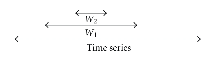
A moving window is run through a time series of data. W₁ is the polynomial fitting window, W₂ is the interpolation window.

Some of the available data series were impossible to smooth with polynomials. They behaved like a typical logistic curve. Hence, the logistic curve was added to the set of functions that could be used to approximate the data:

$$L\left(t\right)=p_0\frac{1+p_1{e}^{p_{3}t}}{1+p_2{e}^{p_{3}t}}.$$ (3)

The parameters W₁ and W₂ and the maximal degree of the polynomials (or logistic curve) were manually selected by visually inspection of the generated curves. The actual degree of the polynomials could vary for each polynomial fitted (thus the curve for a time series of a certain metabolite consists of polynomials of different degrees chained together): for each W₁ window the polynomial giving the least amount of outliers was selected. Data points were identified as outliers when the difference between the measured value and the estimated value was larger than 5% of the range of the response variable. Table 3 summarized the fitting parameters used for each metabolite.

Table 3.

Parameters for the polynomial fitting of the different time series. W₁ is expressed in fraction of the time between the first measurement and the last measurement. W₂ is expressed as a fraction of W₁. PD is the highest degree a polynomial may have; an L is displayed if the data were fitted to a logistic curve.

	C→N limitation			N→C limitation
	W1	W2	PD	W1	W2	PD
GLC	0.40	0.87	5	0.35	0.45	3
NH3	0.50	0.80	2	1	1	L
PiOH	0.70	0.75	5	0.45	0.80	4
O2	0.18	0.90	7	0.11	0.90	7
CO2	0.12	0.90	4	0.12	0.90	7
Ac	0.70	0.88	5	0.15	0.70	3
Lac	1	1	7	0.41	0.80	7
Pyr	0.40	0.80	6	1	1	L
Suc	0.40	0.80	6	0.82	0.99	5
Biomass	0.50	0.70	8	0.37	0.80	4

The polynomial or logistic functions yield a smoothed time profile of the concentrations and enable to calculate the derivative of the concentrations to time. However, when calculating this derivative directly by symbolically deriving the function and filling in the time for the point of interest, one sometimes obtains unrealistically high values (D₁ in Figure 2). Therefore, the derivative was approximated by taking the slope of the point of interest and the previous point on the polynomial (D₂ in Figure 2).

Figure 2.

Two ways of estimating the derivative in point a: D₁ is calculated by symbolically deriving the function in point a; D₂ is the slope between point a and point b (where a and b are calculated from the curve). Dots represent sample points through which a curve is fitted.

The derivative can subsequently be used in (1) to calculate the cellular production (or consumption) fluxes:

$$r_p=\frac{\text{d}C}{\text{d}t}-D\left(C_{\text{in}}-C\right).$$ (4)

Once r_p has been calculated, classical MFA techniques (as described in [4]) can be applied at each time point. The results of those models, evaluated at the different time points, can then be combined to obtain a time profile of internal fluxes.

3.3. Growth Rate Calculation

During the transient period, the assumption that the growth rate is equal to the dilution rate does not hold. However, (4) can explicitly be rewritten for the following biomass:

$$r_{p,\text{Biom}}=\frac{\text{d}{C}_{\text{Biom}}}{\text{d}t}+D{C}_{\text{Biom}}$$ (5)

from which the growth rate can be calculated as

$$\mu =\frac{r_{p,\text{Biom}}}{C_{\text{Biom}}}=\frac{\text{d}{C}_{\text{Biom}}}{\text{d}t}\frac{1}{C_{\text{Biom}}}+D.$$ (6)

4. Results

4.1. Polynomial Fitting

The polynomials fitted through the data (Figures 3 and 4) are used to obtain the concentration, C, and the derivative of the concentration to the time, dC/dt, in each point. From those values, the conversion rate can be calculated (4). Biomass concentrations were calculated from OD values, after generating a calibration curve between cell dry weight (CDW) and OD values. This calibration curve was generated at the end of each experiment. As the curves for both experiments were very close to each other, no distinct calibration was used for the C-limited and N-limited conditions.

Figure 3.

Polynomial fit of some metabolites (expressed in g/L) for the experiment where carbon-limiting medium was replaced with nitrogen-limiting medium. The switch is made at time zero, when the cells are in carbon-limited steady state. Steady state values of five residence times before the switch and five residence times after the switch are not shown.

Figure 4.

Polynomial fit of some metabolites (expressed in g/L) for the experiment where nitrogen-limiting medium was replaced with carbon-limiting medium. The switch is made at time zero, when the cells are in nitrogen-limited steady state. Steady state values of five residence times before the switch and five residence times after the switch are not shown.

The steady state concentration of NH₃ during N-limitation in the C- to N-limitation experiment is around 0.2 g/L (data are not shown on Figure 3, as this value falls out the time frame shown), while it is 0.1 g/L in the N to C-limitation case. These values are high compared to what is found in the literature for the residual nitrogen concentration in similar strains [29] and the nitrogen measurement kit used is probably not suitable for accurately measuring very low NH₃ concentrations.

4.2. Growth Rate and Biomass Production

At time zero, the influent medium was simply switched. No cells were extracted and resuspended in the other medium, as done in [32]. Thus at the switch of the limiting compound, there is an abundance of both, as the medium limited in carbon is saturated with nitrogen while the medium limited in nitrogen is saturated with glucose. In the C to N-limitation experiment, it seems as if N-limitation is reached not much later than when carbon abundance starts (Figure 3). In the N to C-limitation case, nitrogen abundance is reached before all the glucose is depleted: after 5 hours, both glucose and nitrogen are not limiting. This can be seen in Figure 4, in the glucose profile. The glucose concentration becomes only zero after 12 hours while the nitrogen concentration already reaches steady state after 5 hours. At the medium switch, as there is excess nitrogen, the growth rate could increase, but apparently E. coli needs some time to adapt to the new conditions. The biomass flux even decreases as nitrogen is added and becomes almost zero (top of Figure 5). Only seven hours after the medium switch, the growth rate increases sharply to attain almost 0.6 h⁻¹ (right part of Figure 5). This increased growth rate coincides with the uptake of all glucose left in the broth (Figure 4).

Figure 5.

Fluxes in mol/L/h of the biomass production. Open symbols are the values as derived from the polynomials with formula 4; closed symbols are values obtained after flux balancing (top). The growth rate in 1/h of the cells during the transients (bottom). Left: C-limitation to N-limitation; right: N-limitation to C-limitation. The first point left of each figure is the steady state value before the medium switch. The last point right on each figure is the steady state value after at least 50 hours. Error bars represent the standard deviations.

Figure 5 depicts the different growth rates during the transient conditions occurring when switching the limiting substrate. The same trends as in the biomass flux (top of Figure 5) can be observed. For the C- to N-limitation case, a sharp increase in growth rate is observed in the beginning, while for the N- to C-limitation the growth rate decreases to almost zero before increasing to 0.6 h⁻¹, not far from the maximal growth rate of 0.7 h⁻¹. In the carbon to nitrogen-limitation case, the maximal possible growth rate is never achieved and after a sharp increase in the beginning to 0.35 h⁻¹ the growth rate decreases.

The sharp increase in growth rate of the cells at the beginning of the medium switch in the C- to N-limitation experiment (left part of Figure 5) is not accompanied by an increased flux through the Krebs cycle (Figure 8, the first hour after the steady state point, labeled with a triangle). An increase in biomass flux does not imply that intracellular fluxes relative to the biomass flux should increase as well. On the contrary, in the beginning the cells are more energy-efficient than during the carbon-limited steady state (left subfigure of Figure 7 shows that the ATP hydrolysis flux relative to the biomass flux is lower in the beginning implying that the maintenance energy requirement is lower). However, very quickly the flux through the glycolysis increases.

Figure 8.

Fluxmap of the glycolysis, penthose phosphate pathway, and citric acid cycle for the experiment where carbon-limiting medium is changed to nitrogen-limiting medium at time zero. The ordinate on each graph represents the flux expressed in mol/mol Biomass/h while the abscissa represents time. The first point left of each figure is the steady state value before the medium switch. The last point right on each figure is the steady state value after at least 50 hours. Error bars represent the standard deviations.

Figure 7.

Fluxes through the ATP hydrolysis reaction (ATPHY reaction): it can be considered as a measure for the maintenance requirement of the cells, as it combines all the futile cycles and ATP hydrolysed in nonspecific reactions. Left: C-limitation to N-limitation; right: N-limitation to C-limitation. The first point left of each figure is the steady state value before the medium switch. The last point right on each figure is the steady state value after at least 50 hours. Error bars represent the standard deviations.

During the switch of limiting substrate from carbon to nitrogen, less oxygen is consumed and less CO₂ is produced than during steady state (Figure 6). In the beginning of the medium switch, a sharp decline in O₂ consumption and CO₂ production is observed. This correlates with the increased growth rate and biomass production rate (Figure 5). For the experiment where nitrogen limitation is switched to carbon limitation, two parts can be observed: in the first period (until five hours), the O₂ consumption rate and CO₂ production rate increase. Then they suddenly decrease (around 7 hours), to steadily increase again until they reach the steady state level. In both experiments, the steady state value of oxygen consumption and carbon dioxide production is around 16 g/mol Biomass/h. This is in accordance with values obtained with a similar strain [4].

Figure 6.

Amount of oxygen consumed (top) and carbon dioxide produced (bottom). Left: C-limitation to N-limitation; right: N-limitation to C-limitation. The first point left of each figure is the steady state value before the medium switch. The last point right on each figure is the steady state value after at least 50 hours. Error bars represent the standard deviations.

The ATP hydrolysis reaction (Figure 7) lumps all the maintenance requirements and futile cycles (as including all the futile cycles in the metabolic model would yield parallel pathways and the system of equations would not be solvable without measuring intracellular fluxes). It can be seen that during the lag phase of the experiment switching nitrogen to carbon-limitation (right part of Figure 7), the ATP maintenance requirement is around 0.6 mol ATP/mol Biom/h, which is high compared to the values found in a similar E. coli [4]. It seems even more unusually high because there is minimal growth during this period. This high ATP requirement in the beginning of the lag phase correlates with a high uptake of glucose (PTS reaction in Figure 9) and an increased flux in the TCA cycle (Figure 9). The somewhat higher steady state ATP flux at the end of the C- to N-limitation (left part of Figure 7) may be due to multiple physiological steady states [33].

Figure 9.

Fluxmap of the glycolysis, penthose phosphate pathway, and citric acid cycle for the experiment where nitrogen-limiting medium is changed to carbon-limiting medium at time zero. The ordinate on each graph represents the flux expressed in mol/mol Biomass/h while the abscissa represents time. The first point left of each figure is the steady state value before the medium switch. The last point right on each figure is the steady state value after at least 50 hours. Error bars represent the standard deviations.

4.3. Central Carbon Metabolism

During the transient in the C- to N-limitation experiment, the fluxes through the glycolysis increase while those through the Krebs cycle decrease. Also an increase in acetate excretion is observed (Figure 8). The opposite is observed in the N- to C-limitation experiment: fluxes through the glycolysis and acetate production decrease while the fluxes through the Krebs cycle increase (Figure 9). The decrease is not linear: at 15 hours the fluxes through the glycolysis reach a minimum to increase again until the steady state values are obtained after the subsequent 5 hours. In the Krebs cycle, the fluxes gradually increase the first five hours (coinciding with the lag phase observed in the biomass production, Figure 5) after which a sharp decline is observed, immediately followed by a gradual increase, peaking at around 15 hours, and then decrease to steady state level. The succinate flux sharply decreases in the beginning of the switch to gradually increase during the lag phase (5 hours) at which point it reaches a value that does not change anymore. The PEPCB flux, which is responsible for replenishing to the Krebs cycle, follows (or predates) this succinate excretion rate. The excretion of pyruvate decreases during the lag phase and then sharply increases again to reach a lower steady state than under N limitation.

The pentose phosphate pathway is entirely driven by the demands in biomass components, and as each flux is expressed relatively to the biomass, to remove the influence of biomass on the flux values, the fluxes of the pentose phosphate pathway do not change, which results in seemingly huge error bars.

5. Discussion

5.1. Fluxes

When going from an nitrogen-limited medium to a carbon-limited one, a lag phase was observed (Figure 5). A hypothesis could be that when more nitrogen becomes available, the cell starts to break down the accumulated glycogen which is redirected to energy metabolism for protein production. As the biomass composition is assumed to be constant in the model, this increased respiration is measured in the off-gas (O₂ and CO₂ fluxes, Figure 6) and propagated in the model to the ATPHY flux (Figure 7). However, the question remains why the cell would degrade glycogen while there is still plenty of carbon available in the environment. Furthermore, the carbon balance data (not shown) do not reflect an increase in carbon output compared to the carbon input.

Another explanation is that ammonia abundance for cells previously grown under ammonia limiting conditions causes a futile cycle of ammonia import and export. Such cycles have been described previously in micro-organisms, although not under the experimental conditions described in this work [34]. Normally bacterial cells are highly resistant to ammonium, and the negative effects of high NH₄⁺ concentrations are due to an enhanced osmolarity or increased ionic strength of the medium and not caused by ammonium itself [35]. But when changing the medium from nitrogen-limitation to carbon-limitation, the environment of the bacteria switches from low NH₄⁺ concentrations to high ones, and it could be that E. coli needs a certain adaptation period. The scavenging active during N-limitation could still be active in the beginning of the transition, resulting in a high influx of ammonia. To counter this, active efflux is needed, draining ATP and explaining the high energetic cost in the beginning of the addition of ammonium (right part of Figure 7).

Such a mechanism has been observed in plants, where NH₄⁺ toxicity is due to the inability of root cells to limit the influx of ammonium. The high cytosolic NH₄⁺ concentration activates the high-capacity and energy demanding ammonium efflux systems. This ammonium efflux can constitute as much as 80% of primary influx, resulting in a futile cycle of nitrogen across the plasma membrane of root cells. This futile cycle imposes a high energetic cost on the cell that is independent of N metabolism and is accompanied by a decline in growth. Plants that are resistant to high ammonium concentrations (e.g., Oriza sativa) limit the influx of ammonium by lowering the polarisation of the cellular membrane. This lowering of membrane polarisation is not observed in Hordeum vulgare, sensitive to ammonium [36].

The lack of growth resulting from adding ammonium to cells that are adapted to ammonium limitation has previously only been observed in cells lacking glnE (giving the gene product ATase, responsible for activating/inactivating glutamine synthetase) while the wild-type E. coli did not show an impaired growth when shifted from ammonium limitation to excess [37, 38]. Furthermore, the lack of growth in glnE mutants could be alleviated in cells constitutively expressing only low levels of glutamine synthetase [37], suggesting that the toxicity of ammonium in this case is not due to NH₄⁺ itself, but maybe to accumulation of glutamine and/or glutamate. Normally, when shifting from ammonium limitation to carbon-limitation, the amount of active glutamine synthetase decreases instantly [39]. Possibly due to the lack of ATase, the enzymatic glutamine synthetase regulation is lost, and only genetic regulation is present. If this would be the case for the strain used in this study, it could explain the long lag phase after the medium switch. The cells survive until enough glutamine synthetase is degraded before they are able to grow again.

Thus it seems as E. coli MG1655, the strain used in this study, has some anomalies in its nitrogen metabolism. It is known that multiple strains are denominated under this name [40]. The strain used in this work originated from the Coli Genetic Stock Center (CGSC) (personal communications from the Netherlands Culture Collection of Bacteria). The NCCB acquired this strain from CGSC prior to 1991. At that time, the strain was sent out as being fnr⁻ . Later it was found that the strain was a mixture of fnr⁺ and fnr⁻ strains (personal communication from Mary Berlyn). For the experiments in this work, it turned out that the fnr⁻ strain was used. More research is needed to find out why this strain does not grow well when NH₄⁺ is added to a nitrogen-limiting environment.

The lag phase found in the N-limitation to C-limitation experiment stands in sharp contrast with the experiment in which the carbon-limiting medium is replaced with the nitrogen-limiting one and thus carbon is added in the beginning of the switch while nitrogen is not yet limiting. The growth rate increases instantly (top of Figure 5). Death and Ferenci [41] demonstrated that during carbon-limitation, sugar regulons are upregulated by internally synthesised sugars. Lequeux et al. [4] observed that under glucose limitation ptsG is upregulated. The results of the experiments described here show that this up-regulation permits the cells to almost instantly increase their growth rate when carbon is added to a carbon-limited culture. The cells grow as fast as possible, until all nitrogen is consumed and thus the glucose concentration in the reactor broth increases around the same time as the nitrogen decreases (Figure 3).

Hence the peak of succinate (and the smaller peak of pyruvate) occurring around 5 hours after the medium switch (Figure 8) could be due to the depletion of ammonium (Figure 3). The high flux through the glycolysis is not stopped quickly enough and the carbon is excreted as pyruvate or diverted to PEPCB to be excreted as succinate.

5.2. Dynamic MFA

The extension of metabolic flux analysis to allow to predict also intracellular fluxes for cells growing under nonsteady state conditions was successfully applied to transient cultures. As raw measurement data are too noisy, smoothing had to be performed prior to the calculation of the exchange rates, needed for solving the metabolic model. An improvement for this smoothing process would be to incorporate more than two points in the calculation of the derivative, to avoid steep derivatives (and thus unrealistic fluxes) caused by the quirks of the higher-order polynomials.

A possible improvement to the model is to allow fluctuations of the biomass composition. However, this should be accompanied with the appropriate measurements such as protein, RNA, DNA, lipid... content of the biomass. The biomass reaction can then be removed from the model and instead the different biomass compounds can be considered as excreted by the cell.

6. Conclusion

This work introduced the concept of dynamic metabolic flux analysis. We demonstrated how to transform extracellular measurement data from dynamic experiments to flux values. It is not always clear in transient experiments whether the decrease in concentration of the extracellular metabolites is due to the cells stopping production and the remaining product diluting out or whether the cells are actively taking up the metabolites. Transforming the extracellular time series of concentrations to flux values can give the answer to that question. Furthermore, those flux values can help to get insight into the intracellular reactions.

The transformation of time series of concentration measurements to flux values is based on differentiation (in the mathematical sense: finding the derivative) of those time series. Differentiation typically amplifies the noise on the data; therefore a noise-reducing step is needed prior to the differentiation. In this work, this was done by polynomial filtering. Selecting the right parameters for this filtering was done manually and produced satisfying results for the case presented. However, a statistically more sound approach may be desirable.

We subsequently applied dynamic metabolic flux analysis on E. coli cultures in which the limiting compound in the medium was changed from nitrogen to glucose or from glucose to nitrogen.

A lag phase occurred when cells adapted to a nitrogen-limiting environment were supplied with nitrogen. During this lag phase of several hours, the ATP demand was high. No clear physiological reason could be given. The only similar case described in literature for E. coli is a glnE knock out, in which case the toxicity was not due to ammonium itself, but to the accumulation of glutamine/glutamate because the down-regulation of glutamine synthetase is not operative (glutamine synthetase is down-regulated by the gene product of glnE). A possible explanation for the long lag phase observed in the N-to-C-limitation experiment could be that sufficient glutamine synthetase has to be degraded so that the accumulation of glutamine/glutamate does not impair growth anymore.

No lag phase occurred when supplying cells adapted to carbon limitation, with carbon. Instead the growth rate increased immediately. However, the highest growth rates were attained in the N to C-limitation experiment and not in the C- to N-limitation one.

References

- 1.van der Heijden RTJM, Heijnen JJ, Hellinga C, Romein B, Luyben KCAM. Linear constraint relations in biochemical reaction systems: I. Classification of the calculability and the balanceability of conversion rates. Biotechnology and Bioengineering. 1994;43(1):3–10. doi: 10.1002/bit.260430103. [DOI] [PubMed] [Google Scholar]
- 2.van der Heijden RTJM, Romein B, Heijnen JJ, Hellinga C, Luyben KCAM. Linear constraint relations in biochemical reaction systems: II. Diagnosis and estimation of gross errors. Biotechnology and Bioengineering. 1994;43(1):11–20. doi: 10.1002/bit.260430104. [DOI] [PubMed] [Google Scholar]
- 3.Romein B. Mathematical modelling of mammalian cells in suspension culture. Delft, The Netherlands: Technische Universiteit Delft; 2001. Ph.D. thesis. [Google Scholar]
- 4.Lequeux G, Johansson L, Maertens J, Vanrolleghem PA, Lidén G. MFA for overdetermined systems reviewed and compared with RNA expression data to elucidate the difference in shikimate yield between carbon- and phosphate-limited continuous cultures of E. coli W3110.shik1. Biotechnology Progress. 2006;22(4):1056–1070. doi: 10.1021/bp060014u. [DOI] [PubMed] [Google Scholar]
- 5.Wiechert W, Möllney M, Petersen S, De Graaf AA. A universal framework for 13C metabolic flux analysis. Metabolic Engineering. 2001;3(3):265–283. doi: 10.1006/mben.2001.0188. [DOI] [PubMed] [Google Scholar]
- 6.Varma A, Palsson BO. Metabolic capabilities of Escherichia coli: I. Synthesis of biosynthetic precursors and cofactors. Journal of Theoretical Biology. 1993;165(4):477–502. doi: 10.1006/jtbi.1993.1202. [DOI] [PubMed] [Google Scholar]
- 7.Baart GJE, Zomer B, de Haan A, et al. Modeling Neisseria meningitidis metabolism: from genome to metabolic fluxes. Genome Biology. 2007;8(7, article R136) doi: 10.1186/gb-2007-8-7-r136. [DOI] [PMC free article] [PubMed] [Google Scholar]
- 8.Schilling CH, Letscher D, Palsson BO. Theory for the systemic definition of metabolic pathways and their use in interpreting metabolic function from a pathway-oriented perspective. Journal of Theoretical Biology. 2000;203(3):229–248. doi: 10.1006/jtbi.2000.1073. [DOI] [PubMed] [Google Scholar]
- 9.Papin JA, Price ND, Wiback SJ, Fell DA, Palsson BO. Metabolic pathways in the post-genome era. Trends in Biochemical Sciences. 2003;28(5):250–258. doi: 10.1016/S0968-0004(03)00064-1. [DOI] [PubMed] [Google Scholar]
- 10.Maertens J, Vanrolleghem PA. Modeling with a view to target identification in metabolic engineering: a critical evaluation of the available tools. Biotechnology Progress. 2010;26(2):313–331. doi: 10.1002/btpr.349. [DOI] [PubMed] [Google Scholar]
- 11.Chassagnole C, Noisommit-Rizzi N, Schmid JW, Mauch K, Reuss M. Dynamic modeling of the central carbon metabolism of Escherichia coli. Biotechnology and Bioengineering. 2002;79(1):53–73. doi: 10.1002/bit.10288. [DOI] [PubMed] [Google Scholar]
- 12.Peercy BE, Cox SJ, Shalel-Levanon S, San K-Y, Bennett G. A kinetic model of oxygen regulation of cytochrome production in Escherichia coli. Journal of Theoretical Biology. 2006;242(3):547–563. doi: 10.1016/j.jtbi.2006.04.006. [DOI] [PubMed] [Google Scholar]
- 13.Varma A, Palsson BO. Stoichiometric flux balance models quantitatively predict growth and metabolic by-product secretion in wild-type Escherichia coli W3110. Applied and Environmental Microbiology. 1994;60(10):3724–3731. doi: 10.1128/aem.60.10.3724-3731.1994. [DOI] [PMC free article] [PubMed] [Google Scholar]
- 14.Mahadevan R, Edwards JS, Doyle FJ., III Dynamic flux balance analysis of diauxic growth in Escherichia coli. Biophysical Journal. 2002;83(3):1331–1340. doi: 10.1016/S0006-3495(02)73903-9. [DOI] [PMC free article] [PubMed] [Google Scholar]
- 15.Luo R-Y, Liao S, Tao G-Y, et al. Dynamic analysis of optimality in myocardial energy metabolism under normal and ischemic conditions. Molecular Systems Biology. 2006;2, article 71 doi: 10.1038/msb4100071. [DOI] [PMC free article] [PubMed] [Google Scholar]
- 16.Segrè D, Vitkup D, Church GM. Analysis of optimality in natural and perturbed metabolic networks. Proceedings of the National Academy of Sciences of the United States of America. 2002;99(23):15112–15117. doi: 10.1073/pnas.232349399. [DOI] [PMC free article] [PubMed] [Google Scholar]
- 17.Lee JM, Gianchandani EP, Eddy JA, Papin JA. Dynamic analysis of integrated signaling, metabolic, and regulatory networks. PLoS Computational Biology. 2008;4(5) doi: 10.1371/journal.pcbi.1000086. Article ID e1000086. [DOI] [PMC free article] [PubMed] [Google Scholar]
- 18.Buchholz A, Hurlebaus J, Wandrey C, Takors R. Metabolomics: quantification of intracellular metabolite dynamics. Biomolecular Engineering. 2002;19(1):5–15. doi: 10.1016/s1389-0344(02)00003-5. [DOI] [PubMed] [Google Scholar]
- 19.Hoque A, Ushiyama H, Tomita M, Shimizu K. Dynamic responses of the intracellular metabolite concentrations of the wild type and pykA mutant Escherichia coli against pulse addition of glucose or NH3 under those limiting continuous cultures. Biochemical Engineering Journal. 2005;26(1):38–49. [Google Scholar]
- 20.Schaub J, Mauch K, Reuss M. Metabolic flux analysis in Escherichia coli by integrating isotopic dynamic and isotopic stationary 13C labeling data. Biotechnology and Bioengineering. 2008;99(5):1170–1185. doi: 10.1002/bit.21675. [DOI] [PubMed] [Google Scholar]
- 21.Novick A, Szilard L. Description of the chemostat. Science. 1950;112(2920):715–716. doi: 10.1126/science.112.2920.715. [DOI] [PubMed] [Google Scholar]
- 22.Lidén G. Understanding the bioreactor. Bioprocess and Biosystems Engineering. 2001;24(5):273–279. [Google Scholar]
- 23.Zinn M, Witholt B, Egli T. Dual nutrient limited growth: models, experimental observations, and applications. Journal of Biotechnology. 2004;113(1-3):263–279. doi: 10.1016/j.jbiotec.2004.03.030. [DOI] [PubMed] [Google Scholar]
- 24.Egli T. On multiple-nutrient-limited growth of microorganisms, with special reference to dual limitation by carbon and nitrogen substrates. Antonie van Leeuwenhoek. 1991;60(3-4):225–234. doi: 10.1007/BF00430367. [DOI] [PubMed] [Google Scholar]
- 25.De Mey M, Lequeux GJ, Beauprez JJ, et al. Comparison of different strategies to reduce acetate formation in Escherichia coli. Biotechnology Progress. 2007;23(5):1053–1063. doi: 10.1021/bp070170g. [DOI] [PubMed] [Google Scholar]
- 26.Jones E, Oliphant T, Peterson P, et al. SciPy: Open source scientific tools for Python. (2001–2007), http://www.scipy.org/
- 27.Pérez F, Granger BE. IPython: a system for interactive scientific computing. Computing in Science and Engineering. 2007;9(3):21–29. [Google Scholar]
- 28.Wang NS, Stephanopoulos G. Application of macroscopic balances to the identification of gross measurement errors. Biotechnology and Bioengineering. 1983;25(9):2177–2208. doi: 10.1002/bit.260250906. [DOI] [PubMed] [Google Scholar]
- 29.Hua Q, Yang C, Baba T, Mori H, Shimizu K. Response of the central metabolism in Escherichia coli to phosphoglucose isomerase and glucose-6-phosphate dehydrogenase knockouts. Journal of Bacteriology. 2003;185(24):7053–7067. doi: 10.1128/JB.185.24.7053-7067.2003. [DOI] [PMC free article] [PubMed] [Google Scholar]
- 30.Nookaew I, Jewett MC, Meechai A, et al. The genome-scale metabolic model iIN800 of Saccharomyces cerevisiae and its validation: a scaffold to query lipid metabolism. BMC Systems Biology. 2008;2, article 71 doi: 10.1186/1752-0509-2-71. [DOI] [PMC free article] [PubMed] [Google Scholar]
- 31.Provost A, Bastin G. Dynamic metabolic modelling under the balanced growth condition. Journal of Process Control. 2004;14(7):717–728. [Google Scholar]
- 32.Atkinson MR, Blauwkamp TA, Bondarenko V, Studitsky V, Ninfa AJ. Activation of the glnA, glnK, and nac promoters as Escherichia coli undergoes the transition from nitrogen excess growth to nitrogen starvation. Journal of Bacteriology. 2002;184(19):5358–5363. doi: 10.1128/JB.184.19.5358-5363.2002. [DOI] [PMC free article] [PubMed] [Google Scholar]
- 33.Narang A, Konopka A, Ramkrishna D. New patterns of mixed-substrate utilization during batch growth of Escherichia coli K12. Biotechnology and Bioengineering. 1997;55(5):747–757. doi: 10.1002/(SICI)1097-0290(19970905)55:5<747::AID-BIT5>3.0.CO;2-B. [DOI] [PubMed] [Google Scholar]
- 34.Russell JB, Cook GM. Energetics of bacterial growth: balance of anabolic and catabolic reactions. Microbiological Reviews. 1995;59(1):48–62. doi: 10.1128/mr.59.1.48-62.1995. [DOI] [PMC free article] [PubMed] [Google Scholar]
- 35.Müller T, Walter B, Wirtz A, Burkovski A. Ammonium toxicity in bacteria. Current Microbiology. 2006;52(5):400–406. doi: 10.1007/s00284-005-0370-x. [DOI] [PubMed] [Google Scholar]
- 36.Britto DT, Siddiqi MY, Glass ADM, Kronzucker HJ. Futile transmembrane NH4+ cycling: a cellular hypothesis to explain ammonium toxicity in plants. Proceedings of the National Academy of Sciences of the United States of America. 2001;98(7):4255–4258. doi: 10.1073/pnas.061034698. [DOI] [PMC free article] [PubMed] [Google Scholar]
- 37.Kustu S, Hirschman J, Burton D, Jelesko J, Meeks JC. Covalent modification of bacterial glutamine synthetase: physiological significance. Molecular & General Genetics. 1984;197(2):309–317. doi: 10.1007/BF00330979. [DOI] [PubMed] [Google Scholar]
- 38.Atkinson MR, Ninfa AJ. Role of the GlnK signal transduction protein in the regulation of nitrogen assimilation in Escherichia coli. Molecular Microbiology. 1998;29(2):431–447. doi: 10.1046/j.1365-2958.1998.00932.x. [DOI] [PubMed] [Google Scholar]
- 39.Friedrich B, Magasanik B. Urease of Klebsiella aerogenes: control of its synthesis by glutamine synthetase. Journal of Bacteriology. 1977;131(2):446–452. doi: 10.1128/jb.131.2.446-452.1977. [DOI] [PMC free article] [PubMed] [Google Scholar]
- 40.Soupene E, van Heeswijk WC, Plumbridge J, et al. Physiological studies of Escherichia coli strain MG1655: growth defects and apparent cross-regulation of gene expression. Journal of Bacteriology. 2003;185(18):5611–5626. doi: 10.1128/JB.185.18.5611-5626.2003. [DOI] [PMC free article] [PubMed] [Google Scholar]
- 41.Death A, Ferenci T. Between feast and famine: endogenous inducer synthesis in the adaptation of Escherichia coli to growth with limiting carbohydrates. Journal of Bacteriology. 1994;176(16):5101–5107. doi: 10.1128/jb.176.16.5101-5107.1994. [DOI] [PMC free article] [PubMed] [Google Scholar]