

Abstract
Protein folding is a fundamental biological process of great significance for cell function and life-related processes. Surprisingly, very little is presently known about how proteins fold in vivo. The influence of the cellular environment is of paramount importance, as molecular chaperones, the ribosome, and the crowded medium affect both folding pathways and potentially even equilibrium structures. Studying protein folding in physiologically relevant environments, however, poses a number of technical challenges due to slow tumbling rates, low concentrations and potentially non-homogenous populations. Early work in this area relied on biological assays based on antibody recognition, proteolysis, and activity studies. More recently, it has been possible to directly observe the structure and dynamics of nascent polypeptides at high resolution by spectroscopic and microscopic techniques. The fluorescence depolarization decay of nascent polypeptides labeled with a small extrinsic fluorophore is a particularly powerful tool to gain insights into the dynamics of newly synthesized proteins. The fluorophore label senses both its own local mobility and the motions of the macromolecule to which it is attached. Fluorescence anisotropy decays can be measured both in the time and frequency domains. The latter mode of data collection is extremely convenient to monitor the nanosecond motions in ribosome-bound nascent proteins, indicative of the development of independent structure and folding on the ribosome. In this review, we discuss the theory of fluorescence depolarization and its exciting applications to the study of the dynamics of nascent proteins in the cellular environment.
Keywords: protein folding, ribosome, fluorescence anisotropy decay, dynamic fluorescence depolarization, dynamics, nascent chain
1. Introduction
Understanding how proteins achieve their native structure is a holy grail of modern biology. Protein folding is a prerequisite for cell function, hence a process of fundamental importance in life science. Given that aberrant folding resulting in misfolding and aggregation is known to be closely linked to several neurodegenerative and brain disorders (e.g., Alzheimer s, Parkinson’s disease and Huntington’s chorea), understanding the underlying principles of protein folding will likely also lead to long-term benefits to human health.
While protein folding has been studied extensively in vitro [1, 2], very little is known about the influence that a nascent protein’s native environment has on its ability to sample conformational space during and after biosynthesis (Fig. 1). The in vivo environment may well alter the flux across different folding routes, the transient and equilibrium chain dynamics, and possibly even the final structure of a newly synthesized protein [3–5]. The main parameters peculiar to the in vivo environment include co-solute effects, molecular chaperones, and the ribosome.
Figure 1.

Schematic representation of (A) in vitro and (B) in vivo protein folding pathways. Protein folding studies in vitro begin from a chemically or temperature induced unfolded ensemble and proceed through folding intermediates to either the native folded structure or misfolded/aggregated states. Protein folding in the cell differs from in vitro folding due to the influence of molecular chaperones, the ribosome and molecular crowding. (C) High resolution three-dimensional structure of the E. coli 70S ribosome (PDB codes 2AVY, 2AW4) [97].
Molecular crowding is a source of local confinement due to excluded volume effects and potential specific and non-specific interactions. The bulk molecular crowding of the cellular environment promotes intra- and intermolecular collapse and reduces the rates of translational diffusion [6–8].
Chaperones interact with nascent proteins co- and post-translationally to prevent misfolding and possibly promote the folding of a protein into its functional form [9–11]. During translation, nascent proteins are often bound to specific chaperones, e.g., trigger factor (TF), DnaJ, and DnaK, in E. coli [12]. TF is a ribosome-associated chaperone located near the ribosomal exit tunnel [13, 14]. This molecular helper provides an interaction site for nascent chains [15, 16], protecting them from proteolytic cleavage [17, 18]. DnaK interacts with nascent chains through a mechanism involving ADP and ATP nucleotide binding and co-chaperones DnaJ and GrpE [19].
The dynamics and folding of nascent proteins emerging vectorially from the ribosome is likely to be affected by the presence of the ribosome itself (Fig. 1C) [20]. Earlier studies proposed that the ribosome acts as a chaperone [21, 22]. The ribosomal exit tunnel, with its unique RNA/protein-rich cavities [23–26] and electrostatic potential [27, 28], accommodates the last ca. 25–40 C-terminal residues of the nascent chain [29]. It provides a unique highly confined environment, which has been proposed [30] and shown [31] to support early secondary structure formation for some sequences [32]. On the other hand, stable tertiary structure formation within the ribosomal exit tunnel is likely prevented by the constrained tunnel environment, which is 80–100 Å long and has an average width of ~20 Å [26]. Once outside the tunnel, there is sufficient space for nascent proteins to undergo larger-scale conformational sampling and assume globular conformations [33, 34]. Here, the electrostatic potential, spatial confinement and chaperone-like activity of the ribosomal RNA-protein surface offers another unique local environment capable of influencing the structure and dynamics of nascent proteins [21, 22, 35].
Given that, in the cell, the earliest stages of a protein’s life determine its ability to adopt a folded and functional conformation, it is desirable to study protein folding, dynamics, and structure from the initial stages of ribosome-assisted translation. Investigations based on antibody binding and proteolytic digestion demonstrated the presence of co-translational protein folding [33, 36, 37]. However, direct higher resolution spectroscopic investigations have been lacking. Biophysical studies of the structure and dynamics of nascent proteins are complicated by the large size of the ribosome and by the local dynamics of all species involved. Methods able to discriminate the conformation of small nascent proteins from that of the very slowly tumbling ribosome are scarce and only partially effective. Recent NMR investigations on ribosome-bound nascent proteins have led to the identification of N-terminal folded domains in large protein constructs. So far, however, NMR has been limited in its ability to unequivocally identify the conformation of the initial 50–70 nascent residues emerging from the ribosomal surface [38–42]. Cryo-electron microscopy (cryo-EM) has yielded interesting low resolution views [15, 43] of nascent proteins, and a recent single-particle cryo-EM study enabled Bhushan et al. to propose the presence of α-helical nascent chains within the ribosomal exit tunnel [44]. This technique is very promising and has rising potential, although it is presently not clear to what extent it will be possible to overcome the challenges posed by the conformational heterogeneity of the frozen nascent chain solutions required for cryo-EM.
Fluorescence anisotropy decays, i.e., the focus of this review, are uniquely suited to yield direct information on the local dynamics of nascent proteins, both inside and outside the ribosomal tunnel. To date, this method has been the only reported technique able to yield information on the dynamics of nascent proteins. It is therefore an important addition to the modest arsenal of available tools to study co-translational protein folding. Application of the frequency domain version of this technique, known as dynamic fluorescence depolarization, to ribosome-bound nascent chains (RNCs) led to the identification of specific local motions (on the ns and sub-ns timescale), some of which are uniquely diagnostic for the presence of independent nascent protein structure on the ribosome (Fig. 2) [45]. Anisotropy decays can also be interpreted within the Lipari-Szabo “model-free” [46, 47] and in-cone wobbling [35] models to gain additional insights into the degree of spatial confinement of each of the detectable local motions. In this work, we review the theory and applications of anisotropy decay analysis, focusing on its application to the study of co- and immediately post-translational protein folding.
Figure 2.
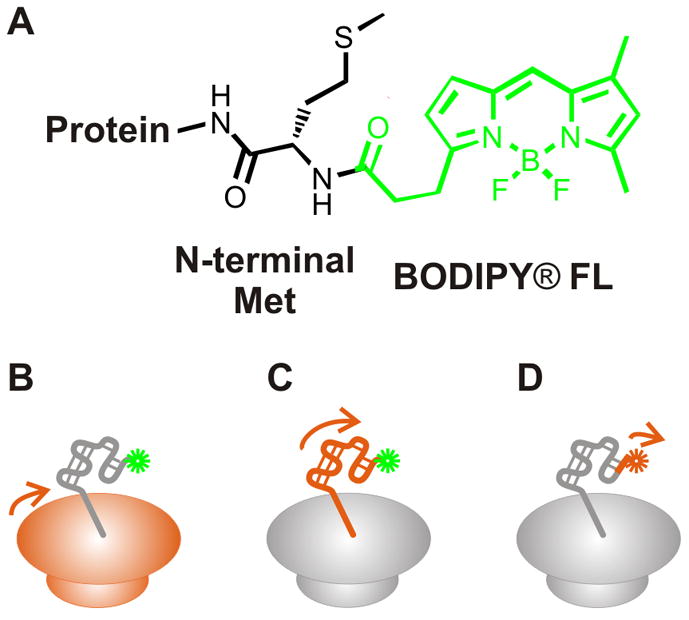
Structure of the BODIPY® FL fluorophore covalently linked to the N-terminus of a protein (panel A). BODIPY® FL is one of several commercially available BODIPY fluorophores that can be used to probe protein dynamics. Fluorescence anisotropy decay measurements via a covalently attached fluorophore report on the (B) global tumbling of the ribosome, (C) the ns motions of the nascent protein, and (D) the fast local motions arising from the fluorophore. The motions described in panels B-D are highlighted in orange.
2. Fluorescence Anisotropy Decay: Description of the Method
2.1. Analysis of Protein Rotational Dynamics by Fluorescence Depolarization
Fluorescence anisotropy decays harbor key information on the global and local rotational dynamics of proteins via the properties of an endogenous or extrinsic fluorophore serving as a reporter for the protein’s motions. The probability that a fluorophore is excited to its electronic singlet state through the absorption of a photon is proportional to cos2θ, where θ is the angle between the absorption transition dipole of the fluorophore and the electric field vector of the incident photon. If a collection of randomly oriented fluorophores is irradiated with polarized light, fluorophores with transition dipoles aligned with the electric field vector of the incoming radiation are preferentially excited, as pictorially shown in Figure 3. This selective excitation is often referred to as photoselection, and it results in partially polarized fluorescence emission [48].
Figure 3.
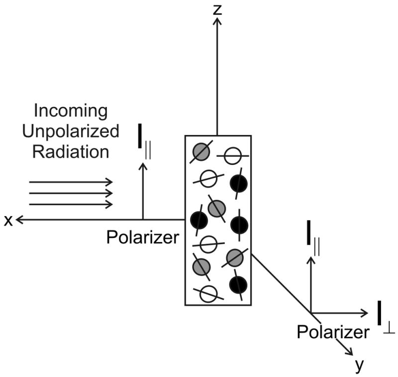
Illumination of a collection of randomly oriented fluorophores with vertically polarized radiation results in the photoselective excitation of fluorophores with transition dipoles aligned with the electric field vector of the polarized light. The fluorophores shown in black are most likely to be excited to the singlet electronic state, while those shaded in gray are less likely to absorb the polarized radiation. The white fluorophores have a very low probability of excitation. Anisotropy is measured my monitoring the vertically (I||) and horizontally (I⊥) polarized components of the emitted fluorescence.
When excitation is induced by irradiation with polarized light, fluorescence emission is also partially polarized due to the photoselective nature of the electronic excitation. The relative polarization of the emitted light can be determined by measuring the intensity of the fluorescent radiation emitted parallel (I||) and perpendicular (I⊥) to the polarization of the excitation beam (Fig. 3).
The extent of depolarization of the emitted light, evaluated independently of the total fluorescence emission intensity (I|| + 2I⊥), is provided by the fluorescence anisotropy r [49], defined as
| (1) |
In a frozen solution containing a collection of immobilized fluorophores, the parallel (I||) and perpendicular (I⊥) intensities of the emitted fluorescence radiation are calculated upon taking into account the cylindrical distribution of excited fluorophores along the z-axis. Given an angle ξ between the absorption and emission transition dipoles, the anisotropy of a frozen collection of fluorophores, known as the fundamental anisotropy r0 [50], is
| (2) |
In the case of liquid solutions, however, the rotational diffusion of the fluorophores occurring on a comparable timescale to the lifetime of the excited electronic state causes a progressive displacement of the emission dipole, leading to depolarization of the emitted radiation. This phenomenon renders the anisotropy smaller than its limiting maximal value expected for a corresponding frozen solution, r0. Therefore, anisotropy decay measurements in liquids provide information about the rotational diffusion of fluorescent molecules [48].
In non-viscous solvents and at physiologically relevant temperatures, the experimentally observable anisotropy of free fluorophores decays to zero rapidly because the fluorophores undergo significant tumbling during the typical 1–10 ns fluorescence lifetimes. This extensive rotation completely depolarizes the emitted radiation. However, when the fluorophore is linked to a larger molecule such as a protein, the observed anisotropy decays significantly more slowly [48].
2.1.1. Steady-State vs. Time-Decay Anisotropy
Fluorescence anisotropy can be observed either in steady-state or decay-resolved data collection modes. In the steady-state mode, sample illumination occurs continuously at constant incident light intensity and fluorescent emission is detected continuously until the desired level of data averaging is achieved. Because the illumination time is significantly longer than the fluorescent lifetime, steady-state analysis yields a time-averaged view of the anisotropy. Steady-state anisotropy measurements provide a powerful tool to determine apparent average macromolecular sizes or to gain qualitative assessments of variations in molecular size and shape. Given its simplicity, steady-state anisotropy is a popular choice to follow a variety of biological processes including protein folding and binding [48].
Anisotropy decay measurements, on the other hand, follow the variations in anisotropy as molecular tumbling depolarizes the initial excitation. For a fluorophore rigidly attached to a spherical macromolecule, the steady-state and decay methods lead, in principle, to the same information. However, anisotropy decay analysis is a required tool to discriminate the presence of distinct motional events. Such events can be detected as long as they occur over the course of the excited state lifetime of the chosen fluorophore reporter. The time dependence of the anisotropy decay [50] is defined as
| (3) |
It can be shown that, for a spherical molecule characterized by a global rotational correlation time τc and single fluorescence lifetime τF, I||(t) and I⊥(t) are
| (4) |
| (5) |
Substitution of equations 2, 4, and 5 into relation 3 yields an expression for the anisotropy decay of a rigid spherical fluorophore-labeled macromolecule displaying a single rotational correlation time
| (6) |
where r(t) is the anisotropy as a function of time, r0 is the fundamental anisotropy at t=0 (prior to any rotational diffusion), and τC is the rotational correlation time of the fluorophore-linked macromolecule. The rotational correlation time is proportional to the size of the macromolecule.
Steady-state anisotropy is mathematically defined as the normalized average of the time-resolved anisotropy, r(t), weighted by the total time-dependent fluorescence emission I(t)
| (7) |
The time averaging process results in the loss of a great deal of the information: steady-state measurements only report on the average motions and are unable to discern the presence of multiple classes of dynamic events [48].
In the case of a fluorophore non-rigidly linked to a macromolecule, anisotropy decay measurements enable the resolution of both the timescales and amplitudes of different motions sensed by the fluorophore. These include local motions of both the fluorophore and the macromolecule, and global tumbling. Therefore, anisotropy decays are a valuable tool to study systems characterized by local flexibility or different domains bearing diverse motional characteristics. For such systems, the anisotropy decay is described as a sum of exponentials reflecting the rotational correlation times and amplitudes of each of the motions, according to
| (8) |
where Fi is the fractional contribution of the i-th anisotropy decay term to the overall anisotropy.
2.2. Anisotropy Decay Analysis in the Time and Frequency Domains
Anisotropy decays can be measured in both the time (TD) and frequency (FD) domains. In TD measurements (impulse response method), the sample is typically illuminated with a laser pulse of much shorter duration than the fluorophore lifetime. The incident light is vertically polarized. The anisotropy decay kinetics is then followed upon monitoring the parallel and perpendicular components of the emitted radiation as a function of time. Several scans are typically collected and summed in time-correlated single photon counting mode [48].
In contrast, the FD approach (harmonic response method) is based on illuminating the sample with continuous radiation of sinusoidally-modulated intensity. The radiation emitted by the fluorophore bears the same intensity modulation profile, but is offset in phase and modulated in amplitude due to the finite lifetime of the fluorophore. Figure 4A provides a diagram of the parameters utilized to determine anisotropy decays in the frequency domain. Initial measurements are carried out under conditions equivalent to the use of unpolarized light (i.e., magic angle polarizer settings) to independently determine the fluorophore lifetime(s) from the phase shift (φ) and modulation (M) as a function of the frequency at which light intensity is modulated (Fig. 4B). The phase shift φ is graphically described in Figure 4A, while M is defined as
Figure 4.

(A) Relationship between excitation and emission radiation in frequency-domain fluorescence spectroscopy demonstrating the origin of experimentally observed quantities. The AC represents the amplitude of the alternating current wave and the DC represents the direct current magnitude for the excitation (solid) and emission (dashed), respectively. The ratio of the AC components of the perpendicular and parallel emission is termed modulation ratio. φ defines the phase shift, while Δφ corresponds to the difference in phase between the perpendicular and parallel emission components. The frequency of the excitation light is constant, while the light intensity modulation frequency is varied in a frequency-domain anisotropy decay measurement. (B) FD fluorescence lifetime raw data, multicomponent fits, and curve fitting residuals for ribosome-bound full-length apoHmpH a prokaryotic globin protein [98]. Following resuspension, ATP (0.5 μM), KCl (100 mM), and the GrpE (0.4 μM) and DnaJ (0.4 μM) chaperones were added to the apoHmpH RNCs.
| (9) |
Depolarization experiments are performed next. At each given light intensity modulation frequency, the phase shift (φ) and AC component (ACEM) of the parallel and perpendicular polarized emission are measured. The phase shift difference Δφ is then calculated [51] as the difference between the phase shifts of the parallel and perpendicular components of the emitted radiation:
| (10) |
The modulation ratio Y [51] is calculated as the ratio of the AC components of the emission intensity:
| (11) |
In FD experiments, several Δφ and Y values are determined over a wide range of light intensity modulation frequencies. Plots of Δφ and Y2 vs. light intensity modulation frequency yield, upon curve fitting, amplitudes and rotational correlation times corresponding to the different components of the anisotropy decay. Obtaining both modulation ratio and phase shift difference data is important to accurately determine the amplitudes and rotational correlation times for the multiple components of the anisotropy decay, as they each weigh the information differently [49].
Anisotropy decay data are typically analyzed by nonlinear least-squares procedures and fit quality is assessed via the reduced χ2 [51]. The FD anisotropy decay parameters can be obtained from the phase shift difference and square of the modulation ratio [52] according to
| (12) |
| (13) |
Equations 12 and 13 illustrate the relationship between Δφ and Y2 and the fundamental anisotropy r0, the light intensity modulation frequency ω (in MHz), rotational correlation time τc, and fluorescence lifetime τ for a single component anisotropy decay. The independently determined fluorophore lifetime is entered into equations 12 and 13. Nonlinear least-squares data fitting is then performed by software packages such as GLOBALS (Laboratory for Fluorescence Dynamics, Irvine, CA) [53], which is an excellent tool to obtain anisotropy decay parameters from experimental FD data.
2.2.1. Relationship between TD and FD Anisotropy Decays
The non-intuitive relationship between fluorescence data collected in the TD and FD are can be understood through the application of Fourier transforms [52, 54]. Accordingly, an intensity decay I(t) measured in the TD can be converted to the frequency domain through calculations of the N and D transforms, defined as
| (14) |
| (15) |
where k denotes either the parallel or perpendicular orientation ω is the linear light intensity modulation frequency in Hz. Ik(t) denotes the polarized TD decays, defined as
| (16) |
| (17) |
where r(t) is given by equation 8 and the unpolarized fluorescence intensity decay I(t) is generally defined as a sum of exponentials.
Nk(ω) and Dk(ω) are related to the phase shift difference and modulation ratio via
| (18) |
| (19) |
An analogous procedure (inverse Fourier transform) may be employed to convert FD data to the TD. However, an alternative simpler route, which does not involve FD data conversion to the TD, is usually followed. The FD data are fit against decay models in the TD via r(t) in relations 16 and 17 (see also relations 6, 8, 20 and 21). The TD expressions for the decay models are then transformed according to relations 14 and 15 and converted to potential FD data-fitting curves via equations 18 and 19. The adjustable parameters of the models (typically rotational correlation times and decay amplitudes) are iteratively varied until minimum deviations from the data are achieved. If desired, one can subsequently generate plots matching the fitted parameters in the more intuitive time domain, to more thoroughly appreciate the results.
In summary, the beauty and power of anisotropy decay measurements in both domains is that they each independently provide all the information needed to calculate the rotational correlation times and amplitudes of the various motions present in the sample, rendering the Fourier-transform-mediated raw data conversion between the two domains unnecessary [55].
2.2.2. Comparison between TD and FD Approaches
Both TD and FD instruments are suitable for measuring anisotropy decays and both types of instruments are commercially available [56]. TD instruments offer the advantages of attaining higher sensitivity for weak fluorescent signals [56] and producing a more intuitive output. While the analog detection of standard FD instruments generally renders them somewhat less sensitive than the single-photon-counting detection systems of comparable TD instruments, FD measurements are capable of providing excellent resolution of multi-component anisotropy decays. It has been argued that this high resolution results from the use of two independent parameters (Δφ(ω) and Y(ω)) to follow anisotropy decays [48] in FD measurements, as opposed to only r(t) in the TD.
In general, both TD and FD instrumentation are suitable for anisotropy decay measurements and each researcher should evaluate and choose the technique to employ based on the needs of the particular research problem.
In the remainder of this review, we will focus primarily on the discussion of anisotropy decays in the frequency domain, though the concepts covered apply equally well to TD and FD anisotropy decays.
2.3. Protein Folding on the Ribosome: Assessing the Local Dynamics of Nascent Proteins by Fluorescence Anisotropy Decays
The experimental assessment of anisotropy decays in systems labeled with an appropriate fluorophore provides access to direct information on the local dynamics of the ribosome-bound protein of interest, providing precious clues about its degree of folding. An important requirement is that the dynamics need to occur on a timescale broadly comparable to the lifetime of the fluorophore. The fluorophore reporter is able to sense both its own local dynamics and the motions of the macromolecule it is connected to. The power of anisotropy decay measurements stems from the fact that the presence of multiple coexisting motions in a macromolecule, responsible for anisotropy decays occurring on sufficiently different timescales, can be separately identified.
2.3.1. Generation of Fluorescently-labeled Ribosome-Bound Nascent Chains
The spectroscopic study of ribosome-nascent protein complexes requires efficient and site-specific fluorophore incorporation, and it is greatly facilitated by the presence of nascent proteins of homogeneous chain length. Due to the inherently stochastic nature of translation, it is impossible to generate a population characterized by all molecules undergoing the same stage of translation, even if translation initiation were made to occur synchronously. Therefore, the analysis described in this review has been carried out primarily on equilibrium populations of stalled chains, rather than in real time during translation.
In order to create stable populations of stalled nascent proteins, the natural SsrA defense of eubacteria against stalled nascent proteins must be disabled [57, 58]. Therefore, anti-SsrA oligonucleotides are usually added to the medium. Ribosome-stalled nascent chains of homogeneous length can be generated primarily by three methods. Truncated mRNA lacking a stop codon can be generated by in vitro transcription of DNA fragments [59] and employed in translation-only cell-free systems, leading to translation halting as the ribosome reaches the mRNA 3′ end. The method has been particularly successful in eukaryotic cell-free systems [31, 60]. Alternatively, truncated mRNA can be generated in situ by deoxyoligonucleotide-directed RNaseH cleavage [61]. Both methods result in the site-specific stalling of translation, leading to homogeneous ribosome-bound chains. The above cell-free procedures offer the advantage of facile control of reaction conditions leading to great flexibility in the introduction of desired components, e.g., molecular chaperones, crowding agents, and unnatural aminoacyl-tRNAs into nascent chains. In addition, one can easily work in excess of mRNA to discourage polysome formation. Alternatively, ribosome stalling can be generated by engineering codons for the 17-residue SecM sequence. Translation halting is promoted by interaction of the SecM translation products with ribosomal proteins facing the interior of the exit tunnel [62, 63]. Notable advantages of constructs generated by this approach are their long-term stability [4, 64] and the straightforward scaling-up of yields if nascent chains are generated in vivo.
Most currently published fluorescence studies addressing protein folding on the ribosome are based on stalled nascent chains generated by in vitro transcription/translation or translation-only cell-free systems. Fluorophores of sufficiently small size can be incorporated co-translationally in these open-vessel media upon addition of unnatural fluorophore-aminoacyl-tRNAs to the transcription/translation mixture [65]. Site-specific incorporation is ensured by the introduction of fluorophore-aminoacyl tRNAs specifically targeting a unique mRNA position, such as derivatives of tRNAfMet, a specific tRNA targeting the production of a unique amino acid (e.g., a single internal lysine) [21, 59, 66] or the tRNAamb suppressor tRNA, which targets the amber codon [66]. Specific details of the in vitro transcription/translation protocol employed by the authors when generating fluorescently labeled RNCs are available in the literature [45]. Fluorescence labeling of in vivo-generated nascent proteins is generally limited by the challenges posed by the poor membrane permeability to conjugated tRNAs. Two alternative solutions exist. Fluorophore-containing unnatural amino acids can be incorporated site-specifically in vivo at amber stop codons [67] in bacterial strains engineered to carry an expanded genetic code and containing both the tRNA and the synthetase specific to the unnatural amino acid. Alternatively, proteins can be engineered to carry a fluorophore-reactive motif, such as a single reactive residue containing an azide or a Cys-rich motif capable of binding the As-containing fluorescein derivative FlAsH [68–70]. Under specific conditions FlAsH is cell-permeable, and it has been successfully used in both FRET and fluorescence anisotropy studies [69, 71].
Methods based on the production of GFP-fusion proteins, which are relatively easy to generate and are widely employed in fluorescence microscopy and spectroscopy [72, 73], are not generally suitable for anisotropy studies on protein folding on the ribosome given the large size of the GFP moiety relative to typical nascent chains. This approach, however, may be a promising avenue for co-translational folding studies on large multi-domain proteins.
Successful anisotropy decay analysis of ribosome-bound nascent chains requires tightly controlled sample preparation conditions to ensure production of pure RNCs. Ultracentrifugation over a sucrose cushion [45], gel filtration chromatography [31], sucrose gradients [43], and affinity chromatography [41] have been employed to purify RNCs from cell-free translation components, including fluorescently labeled aminoacyl-tRNAs. The population and purity of RNCs can be assessed via fluorescence-detected SDS-PAGE.
Researchers conducting fluorescence experiments on ribosome-bound proteins must employ proper controls to ensure the stability of the RNCs throughout the course of the measurements. RNC integrity can be visualized by SDS-PAGE upon the addition of a ribosome release agent such as puromycin [74] or hydroxylamine [75]. It is crucial that these control experiments are conducted on the sample after fluorescence data acquisition is complete to confirm RNC integrity throughout the experiment [45].
2.3.2. Analysis of Multicomponent Fluorescence Anisotropy Decays of Nascent Chains
The local and global motions of a complex fluorophore-labeled macromolecule are characterized by two key parameters: apparent rotational correlation times and fractional contributions to the anisotropy decay (eqn. 8). The former describes the rate of the motion, given the apparent rotational correlation time is proportional to the tumbling time of any given dynamic unit. The latter provides information about the amplitude of the motion, i.e., its degree of spatial confinement. Rotational correlation times and amplitudes of motion are important because they provide crucial information on the presence or absence of independent structured regions in complex macromolecules in solution. For instance, the identification of peculiar local motions has been linked to the existence of individual domains [76] and the presence or absence of independently folded regions in macromolecules [77–79] under solution conditions often inaccessible to other spectroscopic techniques such as X-ray crystallography, cryo-electron microscopy or nuclear magnetic resonance.
In practice, the number of anisotropy decay components that can be explicitly resolved is limited by the accuracy and sensitivity of the measurements as well as by the differences in the amplitudes and rotational correlation times of the different decay components [56, 80, 81]. Lakowicz et al. investigated the ability to discriminate multiple fluorescence lifetime components in the FD for various levels of data confidence [82]. They found that the level of random error is the most critical factor affecting the ability to resolve multiple lifetimes. This study shows that, given 0.5% and 0.1% random errors in the data, exponential components with decay times differing by 40% and 20% can be resolved, respectively. Bearing the above limitations in mind and allowing for additional safety margins, FD anisotropy decay analysis performed with modern commercially available instrumentation is typically regarded as capable of discriminating up to three timescales of motion with rotational correlation times differing by at least a factor of five.
2.3.2.1. Identification of Multicomponent Motions and Determination of Independent Rotational Correlation Times
2.3.2.1.1. Theory
The anisotropy decays of RNCs have peculiar features that differentiate them from typical data collected on individual proteins or smaller macromolecular complexes. Figure 5 illustrates these differences by providing a simulation of the TD anisotropy decays of an RNC and a ribosome-released protein (panel A). This figure also shows raw FD depolarization data collected on the same species (panel B). Section 3 provides practical examples of simulated data profiles while this section focuses primarily on the formal description of the expected multi-component anisotropy decays of RNCs.
Figure 5.
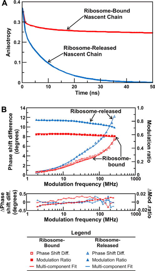
(A) Time-domain simulation illustrating the influence of the slow global tumbling of the ribosome on the observed anisotropy decay. Slow global tumbling prevents the anisotropy of ribosome-bound nascent chains from decaying to zero throughout the ns lifetime of the fluorophore. The anisotropy decays of nascent proteins released from the ribosome decay to zero within 50 ns. All simulations were performed with the Vinci software (ISS, Urbana Champaign). (B) Fluorescence depolarization raw data, multicomponent fits, and curve fitting residuals for ribosome-bound and ribosome-released full-length apoHmpH. The fit parameters derived from this FD anisotropy measurement are shown in Table 1.
The formal features of the fluorescence anisotropy decay of ribosomal complexes are best described via examples from the literature. A recent study by Ellis et al. [45] identifies the presence of independent local dynamics in RNCs site-specifically labeled with a BODIPY® FL (Invitrogen, Carlsbad, CA) fluorophore at their N-terminus. Nascent chains of increasing length corresponding to the sequence of the soluble single-domain protein apomyoglobin and the natively unfolded protein PIR were selected for this study. In the specific case of RNCs bearing fairly long nascent chains emerging out of the ribosomal tunnel, the authors observed peculiar ns timescale motions. Such motions were not detected for short nascent chains (16–35 residues) buried inside the ribosomal tunnel nor for the folding-incompetent natively unfolded sequence PIR.
Nanosecond motions are extremely important, as they provide evidence for the presence of an independent nascent chain conformation, indicative of either a rigid structure or a partially folded species. Consistent with this idea, typical soluble native and molten globular protein domains are known to tumble on the ns timescale [48, 83–85].
The 2-component anisotropy decay of globally unstructured nascent chains is generally described by:
| (20) |
where Fs represents the fraction of anisotropy decay due to the slow ribosomal tumbling, τc,s is the rotational correlation time of the slow ribosomal tumbling, FF represents the fraction of depolarization due to the fast local motions of the fluorophore, and τc,F defines the rotational correlation time of the fast (sub-ns) local motions of the fluorescent probe.
In practice, data are formally fitted to equation 20, but a very large value needs to be imposed to the unresolvable rotational correlation time of the ribosome (e.g., 1 μs) for the fits to converge reproducibly. Therefore, only an apparent single exponential decay is observed, given that global motions of the entire ribosomal complex take place on a timescale much longer than the lifetime of the BODIPY fluorophore. On the other hand, the presence of the extremely slow (≥μs) unresolvable tumbling of the ribosome and its tendency to confine the remaining detectable motions are implied by the fact that the anisotropy does not completely decay to zero and a significant residual fraction of undecayed anisotropy, FS, is observed. This fraction is treated as an adjustable parameter upon data fitting, together with FF and τc,F.
RNCs bearing peptides with independent structure, i.e., apomyoglobin polypeptides exceeding 57 residues in length, were found to exhibit 3-component anisotropy decays described by:
| (21) |
The variables in equation 21 are defined as those in equation 20, with the addition of the FI and τc,I terms to account for the fraction of depolarization and rotational correlation time due to the intermediate timescale motions, respectively. In this case, the fluorophore reports the timescale and amplitude of both its fast local motion and the intermediate timescale motion of the structured polypeptide chain, while the slow ribosomal tumbling is kept fixed, as in the case of the 2-component decays.
As discussed in section 2.2, anisotropy decays can be measured in both the time and frequency domains. Figure 6 provides a cartoon depiction of the global, intermediate, and fast tumbling motions of the RNC complexes and illustrates simulated 2- and 3-component anisotropy decays in both the FD and TD. Discriminating between the presence of 2- and 3-component anisotropy decays was crucial to assess the presence of dynamics due to independent structure in RNCs.
Figure 6.

The presence of one (panel A) or two (panel B) local motions can be discerned from the anisotropy decay of a fluorophore-labeled ribosome-bound nascent protein (RNC). Panels A and B illustrate the physical models underlying 2- and 3-component anisotropy decays of RNCs. In both cases, the slow global tumbling of the ribosome cannot be explicitly resolved. A 2-component decay corresponds to the presence of the local motion of the fluorophore in addition to the slow ribosomal tumbling, while a 3-component decay introduces an intermediate timescale motion diagnostic of protein folding on the ribosome. Panels C and D present simulated 2- and 3-component anisotropy decays in the time and frequency domains, respectively. Dashed and solid lines denote modulation ratios and phase shift differences, respectively. The 2-component anisotropy decays were simulated for a system with FS = 0.7, τS = 1000 ns, FF = 0.3, and τF = 0.3 ns. The parameters of the 3-component anisotropy decay simulations were set to FS = 0.7, τS = 1000 ns, FI = 0.1, τI = 7 ns, FF = 0.2, and τF = 0.3 ns. r0 was fixed at 0.37 for all simulations.
The 2-component anisotropy decay in the time-domain presented in Figure 6C illustrates the fact that the fast motion component leads to an initial rapid decrease in the anisotropy. The anisotropy is prevented from decaying to zero by the rotational restriction imposed by the slow ribosomal tumbling. The presence of a third component in the anisotropy decay is due to an additional ns-timescale local motion. In the TD, each decay component gives rise to an independent exponential decay, with faster decays reflecting small rotational correlation times, and overall vertical amplitudes for each motion reflecting their fractional contribution.
Figure 6D shows the same 2- and 3-component decays in the frequency domain. Upon visual inspection, the presence of an intermediate timescale motion causes the phase shift difference at intermediate light intensity modulation frequencies to increase, giving rise to a “bump” in the data profile. This “bump” is a key spectroscopic signature indicating the presence of an intermediate timescale motion.
2.3.2.1.2. Practical Aspects
In practice, decisions regarding kinetic models that best fit the data are made upon comparing reduced χ2 values. The reduced χ2 provides a measure of the agreement between experimental data and curve fits [82], and is defined as
| (22) |
where Δφω, Yω, Δφcω, and Ycω are the experimental and calculated (see equations 18 and 19) phase shift differences and modulation ratios, respectively, n is the number of experimental light intensity modulation frequencies, f is the number of free-floating parameters in the least-squares analysis, and δΔφ and δY are the uncertainties in phase shift difference and modulation ratio. The last two parameters are hard to estimate and are typically set to 0.2° and 0.004, respectively [51].
Low reduced χ2 values are best. Often, reduced χ2 ~1 is considered ideal and reduced χ2 ≫ 1 is regarded as indicative of either an inadequate model or a systematic error. However, given that the reduced χ2 output depends on a user-input estimate of δΔφ and δY, the absolute value of the reduced χ2 cannot be regarded as the sole determinant to select appropriate data-fitting models [82]. Rather, the relative decrease in reduced χ2 upon switching between different models (usually from a simpler to a more complex model) is a more reliable reporter [54].
In practice, viable kinetic models are first identified from small residuals that are randomly distributed about zero [82]. Residuals are defined as the deviation between curve fits and individual data points. The reduced χ2 criteria discussed above further aid in the selection of the most appropriate kinetic model. As representative examples, Ellis et al. [45] and Lakowicz et al. [54] found that reduced χ2 improvements by a factor > 2.5 and > 2, respectively, justify the choice of a 3-component, over the simpler 2-component, kinetic model.
Figure 5B and Table 1 show additional data that further illustrate the above strategies for the bacterial globin apoHmpH. The apoHmpH RNC encoding the full-length protein sequence is best described by a 3-component anisotropy decay, as evidenced by a significant decrease in reduced χ2 (by a factor >2.5) upon fitting with 3 decay components. The ribosome-released species displays a 2-component anisotropy decay: one component describes the tumbling of the folded protein, while the fast rotational component is attributed to the local motion of the fluorophore label.
Table 1.
Rotational correlation times, fractional amplitudes and reduced χ2 resulting from curve-fitting of the data in Figure 5B.
| Polypeptide Chain | Regimes of Motion |
|||||||
|---|---|---|---|---|---|---|---|---|
| Slow |
Intermediate |
Fast |
Reduced χ2 |
|||||
| Fraction | τC (ns) | Fraction | τC (ns) | Fraction | τC (ns) | 2-comp | 3-comp | |
| Ribosome-bound apoHmpH | 0.41 | 1000 | 0.19 | 1 | 0.40 | 0.05 | 9.74 | 0.34(*) |
| Ribosome-released apoHmpH | n.a. | n.a. | 0.42 | 11 | 0.58 | 0.5 | 0.58(*) | 0.52 |
Bold reduced χ2 values denote the preferred kinetic model.
In order to further justify/disprove the use of a complex kinetic model, it is helpful to critically assess rotational correlation times and fractional amplitudes. The presence of two very similar rotational correlation times or a component with a fractional amplitude that approaches zero is often diagnostic of a fit that utilizes too many exponential decay components [82].
The nonlinear least-squares method is an appropriate routine to fit FD anisotropy decay data. To illustrate this point, we applied least-squares analysis to the simulated FD data of section 3 and proved that the expected rotational correlation times and fractional amplitudes are recovered (Supporting Information).
As discussed in section 2.3.1, fluorescence-detected SDS-PAGE is a method of choice to ensure the absence of undesired contaminants in RNC samples. Anisotropy decay parameters such as those of Table 1 provide additional supporting evidence for the lack of sample contamination by fluorescently labeled aminoacyl-tRNA. The observed anisotropy decays lack a rotational correlation time of ca. 144 ns, i.e., the value ascribed to the global tumbling of aminoacyl tRNA [49].
2.3.2.2. Determination of the Spatial Confinement of Local Nascent Chain Motions: Order Parameters and Cone Semiangles
In addition to information about rotational correlation times of local and global motions, anisotropy decays encode additional useful information about the degree of spatial confinement of the different motions. Interpretation of fluorescence anisotropy decay data via the Lipari-Szabo approach [46] assigns an order parameter to each local motion based on its fractional contribution to the anisotropy decay (see preexponential factors in equations 20 and 21). The order parameter ranges from 0 to 1 and provides a “model-free” measure of the spatial confinement of each local motion. Highly spatially constrained motions are described by an order parameter near 1, while spatially unbiased tumbling is characterized by an order parameters near 0. This parameter is particularly important in the case of co-translational protein folding, given that nascent chains emerging from the ribosome are expected to be significantly spatially confined as a result of the biases imposed by the ribosomal exit tunnel, the ribosome’s outer surface, and the potential presence of ribosome-associated molecular chaperones. Lipari and Szabo originally applied the theory to the characterization of fluorescence decay from a fast, yet restricted, local motion and a slow global macromolecular motion [46]. Specifically, the method was utilized to analyze the depolarization of fluorophores within lipid membranes. The theories have also been applied generally to other highly confined local motions [47]. Order parameters provide an extremely useful measure of the relative dynamics of individual local motions.
The general applicability of the Lipari-Szabo analysis descends from the fact that it does not depend on the specific model of the probe motions; it is “model-free.” It does require five key, but often easily satisfied, assumptions on the nature of the system (Fig. 7): (i) The fluorophore needs to have axial symmetry. (ii) Either the fluorescence absorption or emission dipole of the fluorophore has to be colinear with the fluorophore symmetry axis. (iii) The local motions are completely random in the plane normal to the macromolecular surface, therefore independent of the azimuthal angle. (iv) Local and global motions are independent of each other. (v) The rotational correlation times for the motions differ by at least one order of magnitude.
Figure 7.
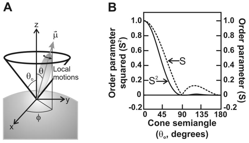
(A) Schematic representation of local (fast, F) and global (slow, S) motions. The local motion is modeled as a vector (μ⃗) colinear with either the emission or excitation dipoles of the fluorophore. The vector is allowed stochastic diffusion via wobbling motions within a static cone defined by semiangle θ0. The x-y component of the dynamics is randomized and therefore independent of the angle φ. In the case of two local motions, the intermediate timescale (I) motions can also be described as wobbling within a static cone defined by a separate semiangle. (B) Graphical representation of the dependence of the order parameter S and its square S2 on the cone semiangle θ0, according to the model of local motions in panel A.
For a system which experiences one slow spatially unrestricted global motion and one fast local motion, the fluorescence anisotropy decay is commonly fit to the multiexponential described in equation 20. Using the model-free approach, the decay can alternatively be represented as:
| (22) |
where SF2 is the squared order parameter for the fast motion. A comparison of equation 20 with equation 22 reveals a simple relation: the fractional amplitude of the slow motion equals the squared order parameter of the fast motion.
The model has been expanded to the case of two independent local motions and one global motion [35]. Here, the fluorescence anisotropy decay can be expressed as
| (23) |
where the subscript I denotes values associated with the intermediate timescale motions. Again, the fractional amplitudes can be related to the order parameters of the fast and intermediate motions, though the relation is not as direct as in the 2-component case. Here, the utility of this analysis is particularly apparent. The model is necessary to clearly distinguish the order parameter of the fast from the intermediate timescale local motion.
Relations 22 and 23 are “model-free” and therefore valid regardless of the exact nature of probe motions. The order parameter can be interpreted further by the application of more specific models (i.e., segmental, diffusive, two-state). A particularly simple and elegant model developed by Kinosita et al. assumes that the probe undergoes stochastic diffusion within a cone bounded by a square-well potential [86]. For the above model, the half angle describing the limiting cone (θ0) can be derived from the order parameter according to
| (24) |
As shown graphically, the order parameter can be clearly related to cone angles describing confinement up to a cone semi-angle of 90° (Fig. 7). A Gaussian-bounded cone model rather than the simpler square-well potential cone resolved the same cone angle values for high values of S2 [87].
Table 2 shows the order parameter and cone semi-angle analysis for the full-length apoHmpH depolarization data of Figure 5B. This analysis is uniquely suited to assess the nascent chain microenvironment, and shows that the ribosome-bound nascent chain is highly spatially confined while exiting the ribosome (rotating within a 28.4° cone semi-angle). The fast (sub-ns) local motions ascribed to the nascent chain’s N-terminal residues and the covalently attached fluorophore are associated with a cone semi-angle of 32.7°, whose value increases upon release from the ribosome.
Table 2.
Order parameter and cone semi-angle analysis illustrating the spatial confinement of the ribosome-bound and ribosome-released full-length apoHmpH nascent chain.
| Polypeptide Chain | Timescales of Motion |
|||||
|---|---|---|---|---|---|---|
| Fast (sub-ns) |
Intermediate (ns) |
|||||
| SF2 | θ0 (degrees) | τC,F (ns) | SI2 | θ0 (degrees) | τC,I (ns) | |
| Ribosome-bound apoHmpH | 0.60 | 32.7 | 0.05 | 0.68 | 28.4 | 1 |
| Ribosome-released apoHmpH | 0.42 | 42.0 | 0.5 | 0 | 0 | 11 |
Ellis et al. performed a systematic analysis of the order parameters and cone semi-angles for the sub-ns motions displayed by the N terminus of sperm whale apomyoglobin and PIR RNCs, as a function of chain length [35]. The authors found that, in both proteins, the motions of the N terminus are highly confined across all the examined chain lengths, but that the exact degree of confinement is sequence and chain length dependent. Interestingly, the degree of confinement of the N terminus varies at different positions within the ribosome exit tunnel. As the nascent protein emerges out of the tunnel, the local mobility of the PIR N terminus was found to progressively increase. However, the mobility of apomyoglobin’s N terminus remains highly constrained as the protein emerges from the ribosome.
3. Analysis of Raw FD Data: Simulations Highlighting the Effect of the System’s Features
The following sections provide computer simulations illustrating how the features of fluorophore-labeled ribosome-bound and ribosome-released nascent chains affect the observed FD data.
3.1. Systems with Two Confined Local Motions and a Slow Non-Resolvable Global Motion
3.1.1. Effect of Rotational Correlation Time on FD Data
Figure 8A illustrates the simulated FD response of a three-component anisotropy decay as the rotational correlation time of the fast sub-ns motion, corresponding to the fast timescale local motions of the fluorophore, is increased from 0.3 ns to 2 ns. As the size of the fluorophore label increases, leading to larger rotational correlation times and a more slowly tumbling fluorophore, the maximum in the phase shift difference profile is reached at lower light intensity modulation frequencies. At low rotational correlation times, the maximum phase shift difference value is not reached within the range of experimentally observable light intensity modulation frequencies. Additionally, the value of the modulation ratio decreases as the rotational correlation time of the fast timescale motion is increased, with the most pronounced increase occurring at higher light intensity modulation frequencies. The simulations in Figure 8A indicate that the location of the maximum in the phase shift difference profile and the value of the modulation ratio, particularly at high light intensity modulation frequencies, are highly sensitive to the rotational correlation time of the fast motion. The raw data profile is therefore expected to vary with the size of the chosen fluorophore label.
Figure 8.

Simulations highlighting the effect of rotational correlation time of the fast (panel A) and intermediate (panel B) timescale motions of a ribosome-bound nascent protein on anisotropy decay data in the frequency domain. The fundamental anisotropy r0 was fixed at 0.37, and the fractional contributions of each rotation were fixed simulation parameters (FS = 0.7, FI = 0.1, FF = 0.2). In panel A, τS was fixed at 1000 ns, τI was fixed at 7 ns, and τF was varied from 0.3 ns to 2 ns. In panel B, τS was fixed at 1000 ns, τF was fixed at 0.3 ns, and τI was varied from 5 ns to 30 ns.
Most importantly, the simulated influence of the apparent rotational correlation time of the ns timescale motion is presented in Figure 8B. These simulations illustrate the impact of co-translational folding on FD data, as the ns timescale motion is diagnostic of independent structure formation. As the rotational correlation time of the intermediate timescale motion increases from 5 ns to 30 ns, the value of the phase shift difference at intermediate light intensity modulation frequencies decreases. Slowing the rotation time of the intermediate motion also results in a decrease in the modulation ratio at low light intensity modulation frequencies. This simulation indicates that the phase shift difference at intermediate light intensity modulation frequencies and the modulation ratio at low light intensity modulation frequencies are most sensitive to the timescale of the intermediate motions. The latter simulations are particularly informative because they illustrate how specific variations in the folding and dynamics of nascent chains can be detected even visually, upon inspection of FD anisotropy decay data.
3.1.2. Effect of Order Parameter on FD Data
As discussed in section 2.3.2.2, the fractional contributions of each timescale of motion provide quantitative insights on the rotational confinement of their respective motions. An increase in freedom of rotation, corresponding to an increase in cone semiangle, is described by a decrease in the squared order parameter S2. Thus, decreasing S2 for the local motions from 0.9 – 0.4 corresponds to increasing the cone semiangle of the local motion. Decreasing the order parameter leads to an increase in phase shift difference at high light intensity modulation frequencies and an increase in modulation ratio at all light intensity modulation frequencies (Fig. 9A). The increase in modulation ratio is most pronounced at light intensity modulation frequencies in the low to intermediate range.
Figure 9.

Simulations highlighting the influence of the rotational restriction of the independent motions of the nascent protein and the local motions of the fluorophore on anisotropy decay data in the frequency domain. The effect of rotational restriction is simulated by ranging the order parameter of the fast (panel A) and intermediate (panel B) timescale motions. The fundamental anisotropy r0 was fixed at 0.37, and the rotational correlation times of each motion were fixed simulation parameters (τS = 1000 ns, τI = 7 ns, and τF = 0.3 ns). In panel A, the fractional contributions of each motion were varied such as to span a range of SF2 from 0.4 to 0.9 (eqn. 23). In panel B, FF was fixed at 0.2 while FS and FI were varied to describe the range of SI2 from 0.4 to 0.9.
In summary, the above simulations indicate that the value of the phase shift difference at high light intensity modulation frequencies is particularly sensitive to the degree of confinement of the local motions of the fluorophore.
The influence of the confinement of the motions of the independently structured ribosome-bound protein on the FD anisotropy decay data is presented in Figure 9B. Decreasing S2 for the intermediate timescale motions from 0.9 to 0.4 causes the phase shift difference to increase at intermediate light intensity modulation frequencies. The modulation ratio at low light intensity modulation frequencies is also sensitive to the increase of rotational freedom observed upon decreasing Si2 from 0.9 to 0.4.
Thus, the modulation ratio at low frequencies and phase shift difference at intermediate frequencies are sensitive to the spatial confinement of the local nascent chain motions imposed by the ribosomal environment.
3.2. Non-Ribosome-Bound Macromolecular Systems
Time-resolved anisotropy decays can also be employed to probe the dynamics of non-ribosome-bound fluorophore-labeled proteins freely diffusing in physiological media. In this case, the timescale and amplitude for both the global and local motions can be explicitly resolved, provided that they occur on a comparable timescale to the lifetime of the fluorophore.
3.2.1. Effect of Rotational Correlation Time
Figure 10A depicts the simulated appearance of a 2-component anisotropy decay in which both components of motion can be explicitly resolved. The plot shows the influence of the rotational correlation time of the local motions of the fluorophore on the appearance of the frequency domain anisotropy decay data. As in the case of a 3-component anisotropy decay (Fig. 8A), increasing the size of the fluorophore tumbling unit causes the maximum in the phase shift difference to appear at lower light intensity modulation frequencies and the modulation ratio to decrease across all light intensity modulation frequencies.
Figure 10.

Simulation of the anisotropy decay of a ribosome released protein illustrating the effect of the rotational correlation time of the fast (panel A) and intermediate (panel B) timescale motions on frequency domain data. The fundamental anisotropy r0 was fixed at 0.37 and the fractional contributions of each rotation were fixed simulation parameters (FI = 0.7, FF = 0.3). In panel A, τI was fixed at 10 ns and τF was varied from 0.3 ns to 3 ns. In panel B, τF was fixed at 0.7 ns and τI was varied from 5 ns to 50 ns.
The latter simulation indicates that the phase shift difference at high light intensity modulation frequencies is sensitive to the timescale of the fast local motions of the fluorophore.
The impact of the rotational correlation time of the global tumbling of the two-component system is investigated in Figure 10B. The data follows the same general trend as Figure 8B, where the rotational correlation time of the intermediate timescale motion was varied. The phase shift difference at high light intensity modulation frequencies decreases with increasing rotational correlation time and the modulation ratio at low light intensity modulation frequencies decreases as the speed of the rotational motion decreases. However, it is clear that the changes in phase shift difference and modulation ratio observed for 2-component decays are much more pronounced than those obtained for 3-component decays.
3.2.2. Effect of Order Parameter
The anisotropy decay data for different degrees of confinement of local fluorophore motions of a ribosome-released nascent protein are presented in Figure 11. As the motion of the fluorophore becomes more spatially restricted (reflected by an increase in order parameter), the maximum in phase shift difference decreases and shifts to lower light intensity modulation frequencies, and the modulation ratio decreases across all frequencies. Therefore, both phase shift differences and light intensity modulation frequencies are sensitive to the confinement of the fast fluorophore motions.
Figure 11.

Simulated effect of the order parameter (degree of rotational restriction) of the fast local fluorophore motions on simulated 2-component anisotropy decays in the frequency domain. The 2-component anisotropy decay is expected for a protein that has been released from the ribosome. The fundamental anisotropy r0 was fixed at 0.37, and the rotational correlation times of each motion were fixed simulation parameters (τI = 10 ns and τF = 0.7 ns). The fractional contributions of each motion were varied such as to span a range of SF2 from 0.4 to 0.9 (eqn. 22).
3.3. Some Notes and Caveats on Data Interpretation
3.3.1. Presence of Multiple Shapes
The single exponential equation 6, relating anisotropy decay and rotational correlation time, applies to a rigid spherical fluorophore or to a rigid macromolecule carrying an embedded fluorophore. However, in case a fluorophore-linked rigid macromolecule is non-spherical, the rotational diffusion is expected to be anisotropic. Under these conditions, the diffusion coefficient assumes tensor properties and the anisotropy decay generally deviates from single-exponential behavior.
Non-spherical molecules can often be effectively modeled as ellipsoids [48], as illustrated in Figure 12. The rotational diffusion coefficient differs around each axis of a general ellipsoid (Fig. 12A) and the anisotropy decay becomes a sum of exponential terms arising from several rotational correlation times which are functions of the rotational diffusion coefficients [48]. Ellipsoids can be classified into two general categories: general ellipsoids with three unique axes (Fig. 12A) and ellipsoids of revolution, characterized by one unique axis and two equivalent axes (Figs. 12B and 12C) [48]. Theory predicts that the anisotropy decay of a general ellipsoid consists of five rotational correlation times. However, given that two pairs of rotational correlation times are similar, the maximum number of observable rotational correlation times has actually been shown to be three [48, 88]. For simplicity, the remainder of this discussion will focus on ellipsoids of revolution, which are subdivided into prolates (with the unique axis longer than the two equivalent axes, Figure 12B) and oblates (with the unique axis smaller than the other equivalent axes, Figure 12C) [48].
Figure 12.

(A) A general ellipsoid features three unique axes a (green), b (red), and c (blue). The anisotropy decay of a general ellipsoid is expected to have multi-exponential character because the rotational diffusion coefficient about each of the three unique axes is different (D1, D2, and D3). (B) Prolate ellipsoids of revolution are characterized by a unique axis (green) which is longer than two axes of equal length (red), while in an oblate ellipsoid of revolution (panel C) the unique axis (green) is shorter than the duplicate axes (red).
The anisotropy decays of ellipsoids of revolution contain only three rotation correlation times. Small and Isenberg performed a systematic analysis on the three expected rotational correlation times of prolate and oblate ellipsoids of different aspect ratios [88].
Oblate ellipsoids of revolution were found to display three nearly identical rotational correlation times at all b/a ratios. Therefore, in practice, rigid oblates are expected to give rise to single exponential anisotropy decays.
On the other hand, the three-component anisotropy decay of prolate ellipsoids was found to include two essentially identical rotational correlation times. In prolates with a/b ratios smaller than ca. 5, the third rotational correlation time is expected to be extremely similar (within 5 ns) to the identical two, while for a/b ratios larger than ca. 5 the third rotational correlation time is larger than the two equivalent ones [88]. Thus, in practice, rigid prolates are expected to display single exponential anisotropy decays except for the case of very elongated shapes. Such shapes are rare for polypeptide chains, as they exceed the most common persistence lengths found in polypeptides, which range between 2 and 5 residues [50]. Elongated shapes are, however, observed in Nature for particular classes of elongated proteins.
In summary, the work by Small and Isenberg showed that it is difficult, if not impossible, to observe multiple anisotropy decays arising from the non-spherical shape of an oblate ellipsoid of revolution and prolate ellipsoids of revolution with a/b ratios less than five. Therefore, the chance to resolve multiple anisotropy decays due to deviations from spherical shape is rare, unless the macromolecule of interest is significantly elongated. However, it is highly desirable to be cautious about the interpretation of multi-component fluorescence anisotropy decays, and be fully aware that their presence may, in some cases, be due to very elongated non-spherical shapes.
3.3.2. Presence of Multiple Populations
It is important to keep in mind that the potential presence of multiple types of fluorophore-labeled species in solution (e.g., multiple conformations of free vs. bound species) needs to be taken into account. The presence of multiple populations may complicate the analysis of anisotropy decays interpreted in terms of local and global motions of one unique population.
In general, it is largely preferable and highly advisable to perform the analysis of nascent protein local conformational dynamics under conditions supporting the presence of only one class of molecules in solution. In addition, wherever possible, one should also perform pertinent calculations and/or carefully chosen control experiments testing whether the observed features of the system depend on the presence of additional populations.
When more than one species is present in solution, the anisotropy decay is expressed as:
| (25) |
where the observed anisotropy decay is the sum of the anisotropy decays of each of the xi components of the system weighted by their fractional populations, assuming Equation 25 is particularly insightful as it shows that even small populations of species characterized by a large anisotropy – arising from slow and/or spatially confined tumbling – can dominate robs(t).
In the case of FD anisotropy decay analysis of complex systems such as ribosome-bound nascent proteins, the potential presence of multiple populations due, for instance, to the interactions of target fluorophore-labeled nascent polypeptides with molecular chaperones, needs to be carefully addressed. Alternatively, one can carry out specific experiments to circumvent the presence of multiple populations. The following example serves to illustrate this point.
The presence of multiple populations due to chaperone-bound and chaperone-free nascent polypeptide species can be prevented by depleting the system of molecular chaperones. The latter species can then be reintroduced one by one in turn to individually assess the effect of each chaperone on the local motions and folding features of nascent proteins. For example, Ellis et al. [45] employed a Δtig cell-free extract to RNCs in the absence of the ribosome-associated molecular chaperone trigger factor (TF). In addition, they also removed any nascent chain-bound DnaK chaperone by the addition of GrpE and excess ATP. DnaK and TF can then be introduced separately to analyze the impact of these chaperones on the anisotropy decay, as illustrated in Figure 13. Data in the absence and presence of chaperones were then compared to gain insights into the influence of each chaperone on the total anisotropy decay. The results of this study indicated that the amplitude of the sub-ns motions corresponding to the rotation of the fluorophore were unaffected by the presence or absence of molecular chaperones.
Figure 13.

Cartoon representations of ribosome-bound nascent polypeptides in the absence and presence of molecular chaperones. (A) In a wild-type cell free system, it is challenging to discern the multiple populations which may arise from various interations with the different chaperones. (B) The challenge of multiple populations can be overcome by employing a Δtig plasmid which lacks trigger factor and flushing the system with GrpE and ATP to eliminate interactions with DnaK to generate a population of chaperone-free RNCs. RNC interactions with chaperones can be then be probed independently by saturating the chaperone-free system with DnaK and trigger factor.
Finally, in some cases it may be possible to explicitly determine or estimate the different populations present in the system. Under such circumstance one can in principle take the different populations into account and fit the observed data to equation 25, where each ri(t) is defined according to equation 20 or 21. Caution must be exercised, as this analysis is only appropriate if the number of adjustable parameters in the data fitting algorithm is low. As an example pertaining to the case of ribosome-bound nascent proteins, known equilibrium constants (or estimated equilibrium constant ranges) may be employed to calculate the expected populations of TF-bound and TF-free nascent chains. This type of analysis was applied to nascent apomyoglobin and showed that, depending on the affinity of TF for the nascent protein, the cone semiangle attributable to some of the chaperone-free nascent chain motions can vary dramatically [35].
4. Beyond the Ribosome: the Timecourse of Nascent Protein Release
The release of nascent proteins from the ribosome is a crucial step in protein expression. In Nature, the mRNA encoding a protein’s amino acid sequence contains a stop codon, which encodes information for polypeptide chain release mediated by release factors [89]. The latter species catalyze the hydrolysis of the peptidyl-tRNA ester bond that links the C-terminus of the nascent protein to the 3′ end of the tRNA. Under physiologically relevant conditions, the rate of ester bond cleavage is of the order of 0.5 s−1 [90]. However, virtually nothing is known about the timescale and mechanism of the subsequent events underlying protein birth, including the protein’s departure from the ribosome, release of any bound molecular chaperones, and any concurrent protein folding.
Assessment of ribosome release in the cell is complicated by the stochastic nature of the process as protein synthesis and release are not synchronized across the entire population of RNCs. To overcome the above challenge, stalled RNCs can be generated by translation of mRNA lacking a stop codon. Translation is halted by oligonucleotides which are complementary to the mRNA sequence beyond the coding region of the desired protein product. The ribosome release of stalled RNCs can then be triggered ad hoc by the addition of release agents such as hydroxylamine or puromycin, which cleave the ester bond linking protein to tRNA [74, 75].
The observed anisotropy decay of an extrinsic fluorophore bound to a nascent protein is highly influenced by the presence of the ribosome (Fig. 14). This property hints at the fact that fluorescence anisotropy can be employed as a tool to study the time course of ribosome release of nascent proteins, corresponding to the crucial steps of a protein’s birth. This fascinating biological question can be addressed by both steady-state and time-resolved anisotropy.
Figure 14.

Fluorescence depolarization raw data, multicomponent fits, and curve fitting residuals for ribosome-bound and ribosome-released PIR90. Release of nascent PIR90 from the ribosome induces the formation of a significantly more dynamic species, as illustrated by the variations in the modulation ratio and phase shift difference profiles.
Analysis of the release of nascent proteins from the ribosome by both steady-state and time-resolved anisotropy may be complicated by the potential presence of multiple populations, in case a fraction of the population of nascent chains experiences interactions with molecular chaperones and/or the ribosome. Additionally, the finite lifetime of the fluorophore and signal-to-noise ratio of the observed data limit the number of rotational correlation times which can be resolved in an anisotropy decay. In order to establish the feasibility of protein birth studies according to the simplest possible scenario, we performed pilot experiments with the natively unfolded model protein PIR. PIR does not interact with molecular chaperones and displays an anisotropy decay featuring only two rotational correlation times, when bound to the ribosome [45]. Figure 15 illustrates preliminary data on the timecourse of ribosome release of PIR following the addition of hydroxylamine. Appropriate control experiments are also shown. Interestingly, under the reported experimental conditions the PIR release process is fairly slow and it displays apparent single exponential kinetics.
Figure 15.

(A) Cartoon illustrating the release of a nascent protein from the ribosome. This process occurs in Nature when the ribosome reaches an mRNA stop codon and appropriate release factors promote nascent chain departure. Ribosome release of nascent proteins can also be triggered ad hoc, upon addition of selected agents to stalled ribosomes. (B) Ribosome-release timecourse for the natively unfolded protein PIR (circles). The chain release process was triggered by the addition of hydroxylamine, which cleaves the ester bond linking the ribosome-associated tRNA to the nascent chain’s C terminus. The observed rate constant for hydroxylamine-induced PIR departure from the ribosome, corrected for minor amounts of spontaneous chain release (see control data, squares) is 1.3 × 10⁻³ s−1. This rate constant shows that, for the selected experimental conditions, PIR ribosome release and any concurrent PIR conformational sampling take place on the hr timescale. The triangles denote the data for a fully ribosome–released hydroxylamine release reaction for one hour at 37°C.
Steady-state anisotropy measurements can provide information on the fractional populations of species present in a system. In general, Weber’s addition law of the polarization of several oscillators [91] states that for a two-state system consisting of two species A and B in which the fluorescent intensities of A and B are identical, the fraction of species A is given by:
| (26) |
where robs is the measured steady-state anisotropy, rA is the steady-state anisotropy of species A, and rB is the steady-state anisotropy of species B [92]. Equation 26 can be applied to studies of ribosome release by defining the two populations as the ribosome-bound and ribosome-released species.
It is worth noting that, in general, the steady-state anisotropy does not directly track populations. Caution must be used in interpreting steady-state anisotropy values in terms of populations, as the observed anisotropy is weighted by the relative fluorescence intensity of each state. Thus, the apparent anisotropy is skewed toward the state with a higher fluorescent intensity. Any observed steady-state anisotropy can be expressed as:
| (27) |
where Xi is the fractional population of species i with intensity fi and anisotropy ri [48].
In Figure 15, steady-state anisotropy was employed to determine the populations of the ribosome-free and ribosome-bound PIR as a function of time, following hydroxylamine addition. The plot shows that the departure of PIR from the ribosome upon release occurs on the ca. one hour timescale and serves to illustrate the feasibility of employing steady-state anisotropy measurements to study ribosome release processes. The data obtained from steady-state anisotropy are especially significant if one performs a parallel analysis of the time course of peptidyl tRNA cleavage monitored by SDS gel. This information enables insights into how the timescale of bond cleavage compares to the time required for the protein to depart from the ribosome, as monitored with steady-state anisotropy.
Anisotropy decays are also additive according to equation 25 and can provide information on the population of multiple species. In addition, anisotropy decays can also yield information on the dynamics of any relevant transient species.
The FD signatures of ribosome-bound and ribosome-released PIR are significantly different (Fig. 14). However, acquiring useful information on species that may become populated during the release requires the timescale of the spectroscopic probe to be negligible relative to the timescale of the process being studied. Thus, the time required to measure the anisotropy decay must be negligible relative to the timescale of ribosome release and protein folding.
Previous studies in both the TD and FD have demonstrated the feasibility of measuring anisotropy decay on a negligible timescale relative to the timescale of protein folding. The key to the success of the aforementioned studies is the difference in the timescales of fluorescence anisotropy decays (ns) and protein folding (μs or greater). Ingersoll and coworkers employed FD multiharmonic Fourier fluorescence spectroscopy to study anisotropy decays of proteins undergoing changes in their conformation and structure throughout the course of 20 to 90 minute processes. This method is capable of simultaneously measuring multiple light intensity modulation frequencies and can therefore yield FD data within 0.1 s [93].
Alternatively, Beechem has reported on a method enabling the direct observation of polarized fluorescence emission decays in the TD [94]. Previous studies have successfully combined direct observation of decays in the TD by multiple time-correlated single-photon counting with stopped-flow technology. These experiments were able to measure several fluorescence decays throughout the course of one folding event [95]. This type of experiment has been successfully applied to study the dynamics of transiently populated protein folding intermediates [83, 95, 96] and offers the potential to provide time-resolved insights into the dynamics of any intermediates which may form as nascent proteins are released from the ribosome and assume their native structure in solution.
It is important to note that stopped-flow technology may not be necessary to study the ribosome release of nascent proteins by anisotropy decay analysis, in case the relevant timescale of ribosome release and folding of newly synthesized proteins is sufficiently long and concentrations are sufficiently high. It may be possible to trigger the release event by manual mixing and spectroscopically follow the process by anisotropy decay measurements in either the TD or FD, as has been reported for previous studies of protein folding.
5. Conclusions
In summary, anisotropy decays provide a powerful tool to resolve the local dynamics of complex systems such as ribosome-bound nascent proteins. This analysis yields valuable insights into the degree of co-translational folding and the confinement imposed by the ribosome on nascent polypeptides by resolving both the timescales and amplitudes for the major sub-ns and ns local motions. As long as proper care is taken to ensure that the samples are comprised primarily of a unique fluorescence-active species, anisotropy decay measurements offer exciting opportunities to understand the intricacies of protein folding on the ribosome and are amenable for extension to the investigation of the influence of other physiologically relevant folding modulators such as molecular chaperones and molecular crowding agents.
Supplementary Material
Acknowledgments
We are grateful to Enrico Gratton for valuable discussions. We thank Daria Fedyukina and Ashok Sekhar for a critical reading of the manuscript. This work was supported by the National Science Foundation (grant MCB-0544182 to S.C.). S.W. was the recipient of a National Institutes of Health Molecular Biophysics Training Fellowship (T32 GM08293).
Footnotes
Publisher's Disclaimer: This is a PDF file of an unedited manuscript that has been accepted for publication. As a service to our customers we are providing this early version of the manuscript. The manuscript will undergo copyediting, typesetting, and review of the resulting proof before it is published in its final citable form. Please note that during the production process errors may be discovered which could affect the content, and all legal disclaimers that apply to the journal pertain.
References
- 1.Englander SW, Mayne L, Krishna MMG. Protein folding and misfolding: mechanism and principles. Q Rev Biophys. 2007;40:287–326. doi: 10.1017/S0033583508004654. [DOI] [PMC free article] [PubMed] [Google Scholar]
- 2.Radford SE. Protein folding: progress made and promises ahead. Trends Biochem Sci. 2000;25:611–618. doi: 10.1016/s0968-0004(00)01707-2. [DOI] [PubMed] [Google Scholar]
- 3.Ellis RJ. The “bio” in biochemistry: Protein folding inside and outside the cell. Science. 1996;272:1448–1449. doi: 10.1126/science.272.5267.1448. [DOI] [PubMed] [Google Scholar]
- 4.Evans MS, Clark TF, Clark PL. Conformations of co-translational folding intermediates. Protein Pept Lett. 2005;12:189–195. doi: 10.2174/0929866053005908. [DOI] [PubMed] [Google Scholar]
- 5.Bartlett AI, Radford SE. An expanding arsenal of experimental methods yields an explosion of insights into protein folding mechanisms. Nat Struct Mol Biol. 2009;16:582–588. doi: 10.1038/nsmb.1592. [DOI] [PubMed] [Google Scholar]
- 6.Ellis RJ, Minton AP. Cell biology - Join the crowd. Nature. 2003;425:27–28. doi: 10.1038/425027a. [DOI] [PubMed] [Google Scholar]
- 7.Ellis RJ. Macromolecular crowding: obvious but underappreciated. Trends Biochem Sci. 2001;26:597–604. doi: 10.1016/s0968-0004(01)01938-7. [DOI] [PubMed] [Google Scholar]
- 8.Homouz D, Perham M, Samiotakis A, Cheung MS, Wittung-Stafshede P. Crowded, cell-like environment induces shape changes in aspherical protein. Proc Natl Acad Sci U S A. 2008;105:11754–11759. doi: 10.1073/pnas.0803672105. [DOI] [PMC free article] [PubMed] [Google Scholar]
- 9.Frydman J. Folding of newly translated proteins in vivo: The role of molecular chaperones. Annu Rev Biochem. 2001;70:603–647. doi: 10.1146/annurev.biochem.70.1.603. [DOI] [PubMed] [Google Scholar]
- 10.Hartl FU, Hayer-Hartl M. Protein folding - Molecular chaperones in the cytosol: from nascent chain to folded protein. Science. 2002;295:1852–1858. doi: 10.1126/science.1068408. [DOI] [PubMed] [Google Scholar]
- 11.Hartl FU, Hayer-Hartl M. Converging concepts of protein folding in vitro and in vivo. Nat Struct Mol Biol. 2009;16:574–581. doi: 10.1038/nsmb.1591. [DOI] [PubMed] [Google Scholar]
- 12.Wegrzyn RD, Deuerling E. Molecular guardians for newborn proteins: ribosome-associated chaperones and their role in protein folding. Cell Mol Life Sci. 2005;62:2727–2738. doi: 10.1007/s00018-005-5292-z. [DOI] [PMC free article] [PubMed] [Google Scholar]
- 13.Baram D, Pyetan E, Sittner A, Auerbach-Nevo T, Bashan A, Yonath A. Structure of trigger factor binding domain in biologically homologous complex with eubacterial ribosome reveals its chaperone action. Proc Natl Acad Sci U S A. 2005;102:12017–12022. doi: 10.1073/pnas.0505581102. [DOI] [PMC free article] [PubMed] [Google Scholar]
- 14.Ferbitz L, Maier T, Patzelt H, Bukau B, Deuerling E, Ban N. Trigger factor in complex with the ribosome forms a molecular cradle for nascent proteins. Nature. 2004;431:590–596. doi: 10.1038/nature02899. [DOI] [PubMed] [Google Scholar]
- 15.Merz F, Boehringer D, Schaffitzel C, Preissler S, Hoffmann A, Maier T, Rutkowska A, Lozza J, Ban N, Bukau B, Deuerling E. Molecular mechanism and structure of Trigger Factor bound to the translating ribosome. EMBO J. 2008;27:1622–1632. doi: 10.1038/emboj.2008.89. [DOI] [PMC free article] [PubMed] [Google Scholar]
- 16.Rutkowska A, Mayer MP, Hoffmann A, Merz F, Zachmann-Brand B, Schaffitzel C, Ban N, Deuerling E, Bukau B. Dynamics of trigger factor interaction with translating ribosomes. J Biol Chem. 2008;283:4124–4132. doi: 10.1074/jbc.M708294200. [DOI] [PubMed] [Google Scholar]
- 17.Hoffmann A, Merz F, Rutkowska A, Zachmann-Brand B, Deuerling E, Bukau B. Trigger factor forms a protective shield for nascent polypeptides at the ribosome. J Biol Chem. 2006;281:6539–6545. doi: 10.1074/jbc.M512345200. [DOI] [PubMed] [Google Scholar]
- 18.Tomic S, Johnson AE, Hartl FU, Etchells SA. Exploring the capacity of trigger factor to function as a shield for ribosome bound polypeptide chains. FEBS Lett. 2006;580:72–76. doi: 10.1016/j.febslet.2005.11.050. [DOI] [PubMed] [Google Scholar]
- 19.Mayer MP, Bukau B. Hsp70 chaperones: Cellular functions and molecular mechanism. Cell Mol Life Sci. 2005;62:670–684. doi: 10.1007/s00018-004-4464-6. [DOI] [PMC free article] [PubMed] [Google Scholar]
- 20.Kramer G, Boehringer D, Ban N, Bukau B. The ribosome as a platform for co-translational processing, folding and targeting of newly synthesized proteins. Nat Struct Mol Biol. 2009;16:589–597. doi: 10.1038/nsmb.1614. [DOI] [PubMed] [Google Scholar]
- 21.Kudlicki W, Coffman A, Kramer G, Hardesty B. Ribosomes and ribosomal RNA as chaperones for folding of proteins. Fold Des. 1997;2:101–108. doi: 10.1016/S1359-0278(97)00014-X. [DOI] [PubMed] [Google Scholar]
- 22.Singh R, Rao CM. Chaperone-like activity and surface hydrophobicity of 70S ribosome. FEBS Lett. 2002;527:234–238. doi: 10.1016/s0014-5793(02)03243-x. [DOI] [PubMed] [Google Scholar]
- 23.Ban N, Nissen P, Hansen J, Moore PB, Steitz TA. The complete atomic structure of the large ribosomal subunit at 2.4 angstrom resolution. Science. 2000;289:905–920. doi: 10.1126/science.289.5481.905. [DOI] [PubMed] [Google Scholar]
- 24.Harms J, Schluenzen F, Zarivach R, Bashan A, Gat S, Agmon I, Bartels H, Franceschi F, Yonath A. High resolution structure of the large ribosomal subunit from a mesophilic Eubacterium. Cell. 2001;107:679–688. doi: 10.1016/s0092-8674(01)00546-3. [DOI] [PubMed] [Google Scholar]
- 25.Wimberly BT, Brodersen DE, Clemons WM, Morgan-Warren RJ, Carter AP, Vonrhein C, Hartsch T, Ramakrishnan V. Structure of the 30S ribosomal subunit. Nature. 2000;407:327–339. doi: 10.1038/35030006. [DOI] [PubMed] [Google Scholar]
- 26.Voss NR, Gerstein M, Steitz TA, Moore PB. The geometry of the ribosomal polypeptide exit tunnel. J Mol Biol. 2006;360:893–906. doi: 10.1016/j.jmb.2006.05.023. [DOI] [PubMed] [Google Scholar]
- 27.Baker NA, Sept D, Joseph S, Holst MJ, McCammon JA. Electrostatics of nanosystems: Application to microtubules and the ribosome. Proc Natl Acad Sci U S A. 2001;98:10037–10041. doi: 10.1073/pnas.181342398. [DOI] [PMC free article] [PubMed] [Google Scholar]
- 28.Lu JL, Deutsch C. Electrostatics in the Ribosomal Tunnel Modulate Chain Elongation Rates. J Mol Biol. 2008;384:73–86. doi: 10.1016/j.jmb.2008.08.089. [DOI] [PMC free article] [PubMed] [Google Scholar]
- 29.Svetlov MS, Kolb VA, Spirin AS. Folding of the firefly luciferase polypeptide chain with the immobilized C terminus. Mol Biol. 2007;41:86–92. [PubMed] [Google Scholar]
- 30.Ziv G, Haran G, Thirumalai D. Ribosome exit tunnel can entropically stabilize alpha-helices. Proc Natl Acad Sci U S A. 2005;102:18956–18961. doi: 10.1073/pnas.0508234102. [DOI] [PMC free article] [PubMed] [Google Scholar]
- 31.Woolhead CA, McCormick PJ, Johnson AE. Nascent membrane and secretory proteins differ in FRET-detected folding far inside the ribosome and in their exposure to ribosomal proteins. Cell. 2004;116:725–736. doi: 10.1016/s0092-8674(04)00169-2. [DOI] [PubMed] [Google Scholar]
- 32.Lu JL, Deutsch C. Folding zones inside the ribosomal exit tunnel. Nat Struct Mol Biol. 2005;12:1123–1129. doi: 10.1038/nsmb1021. [DOI] [PubMed] [Google Scholar]
- 33.Frydman J, Erdjument-Bromage H, Tempst P, Hartl FU. Co-translational domain folding as the structural basis for the rapid de novo folding of firefly luciferase. Nat Struct Biol. 1999;6:697–705. doi: 10.1038/10754. [DOI] [PubMed] [Google Scholar]
- 34.Nicola AV, Chen W, Helenius A. Co-translational folding of an alphavirus capsid protein in the cytosol of living cells. Nat Cell Biol. 1999;1:341–345. doi: 10.1038/14032. [DOI] [PubMed] [Google Scholar]
- 35.Ellis JP, Culviner PH, Cavagnero S. Confined dynamics of a ribosome-bound nascent globin: Cone angle analysis of fluorescence depolarization decays in the presence of two local motions. Protein Sci. 2009;18:2003–2015. doi: 10.1002/pro.196. [DOI] [PMC free article] [PubMed] [Google Scholar]
- 36.Evans MS, Sander IM, Clark PL. Cotranslational Folding Promotes beta-Helix Formation and Avoids Aggregation In Vivo. J Mol Biol. 2008;383:683–692. doi: 10.1016/j.jmb.2008.07.035. [DOI] [PMC free article] [PubMed] [Google Scholar]
- 37.Clark PL, King J. A newly synthesized, ribosome-bound polypeptide chain adopts conformations dissimilar from early in vitro refolding intermediates. J Biol Chem. 2001;276:25411–25420. doi: 10.1074/jbc.M008490200. [DOI] [PubMed] [Google Scholar]
- 38.Cabrita LD, Hsu STD, Launay H, Dobson CM, Christodoulou J. Probing ribosome-nascent chain complexes produced in vivo by NMR spectroscopy. Proc Natl Acad Sci U S A. 2009;106:22239–22244. doi: 10.1073/pnas.0903750106. [DOI] [PMC free article] [PubMed] [Google Scholar]
- 39.Hsu STD, Cabrita LD, Fucini P, Christodoulou J, Dobson CM. Probing Side-Chain Dynamics of a Ribosome-Bound Nascent Chain Using Methyl NMR Spectroscopy. J Am Chem Soc. 2009;131:8366-+. doi: 10.1021/ja902778n. [DOI] [PubMed] [Google Scholar]
- 40.Hsu STD, Fucini P, Cabrita LD, Launay H, Dobson CM, Christodoulou J. Structure and dynamics of a ribosome-bound nascent chain by NMR spectroscopy. Proc Natl Acad Sci U S A. 2007;104:16516–16521. doi: 10.1073/pnas.0704664104. [DOI] [PMC free article] [PubMed] [Google Scholar]
- 41.Rutkowska A, Beerbaum M, Rajagopalan N, Fiaux J, Schmieder P, Kramer G, Oschkinat H, Bukau B. Large-scale purification of ribosome-nascent chain complexes for biochemical and structural studies. FEBS Lett. 2009;583:2407–2413. doi: 10.1016/j.febslet.2009.06.041. [DOI] [PubMed] [Google Scholar]
- 42.Christodoulou J, Larsson G, Fucini P, Connell SR, Pertinhez TA, Hanson CL, Redfield C, Nierhaus KH, Robinson CV, Schleucher J, Dobson CM. Heteronuclear NMR investigations of dynamic regions of intact Escherichia coli ribosomes. Proc Natl Acad Sci U S A. 2004;101:10949–10954. doi: 10.1073/pnas.0400928101. [DOI] [PMC free article] [PubMed] [Google Scholar]
- 43.Gilbert RJC, Fucini P, Connell S, Fuller SD, Nierhaus KH, Robinson CV, Dobson CM, Stuart DI. Three-dimensional structures of translating ribosomes by cryo-EM. Mol Cell. 2004;14:57–66. doi: 10.1016/s1097-2765(04)00163-7. [DOI] [PubMed] [Google Scholar]
- 44.Bhushan S, Gartmann M, Halic M, Armache JP, Jarasch A, Mielke T, Berninghausen O, WIlson DN, Beckmann R. Nat. Struct. Mol. Biol. Advance Online Publication. 2010 doi: 10.1038/nsmb.1756. [DOI] [PubMed] [Google Scholar]
- 45.Ellis JP, Bakke CK, Kirchdoerfer RN, Jungbauer LM, Cavagnero S. Chain dynamics of nascent polypeptides emerging from the ribosome. ACS Chem Biol. 2008;3:555–566. doi: 10.1021/cb800059u. [DOI] [PMC free article] [PubMed] [Google Scholar]
- 46.Lipari G, Szabo A. Effect of Librational Motion on Fluorescence Depolarization and Nuclear Magnetic-Resonance Relaxation in Macromolecules and Membranes. Biophys J. 1980;30:489–506. doi: 10.1016/S0006-3495(80)85109-5. [DOI] [PMC free article] [PubMed] [Google Scholar]
- 47.Lipari G, Szabo A. Model-Free Approach to the Interpretation of Nuclear Magnetic-Resonance Relaxation in Macromolecules .1. Theory and Range of Validity. J Am Chem Soc. 1982;104:4546–4559. [Google Scholar]
- 48.Lakowicz JR. Principles of Fluorescence Spectroscopy. 3. Springer; New York: 2006. [Google Scholar]
- 49.Jameson DM, Hazlett TL. Time-Resolved Fluorescence in Biology and Biochemistry. In: Dewey TG, editor. Biophysical and Biochemical Aspects of Fluorescence Spectroscopy. Plenum Press; New York: 1991. pp. 105–133. [Google Scholar]
- 50.Cantor CR, Schimmel PR. Biophysical Chemistry. WH Freeman and Company; New York: 1980. [Google Scholar]
- 51.Ross JA, Jameson DM. Time-resolved methods in biophysics. 8. Frequency domain fluorometry: applications to intrinsic protein fluorescence. Photochem Photobiol Sci. 2008;7:1301–1312. doi: 10.1039/b804450n. [DOI] [PubMed] [Google Scholar]
- 52.Weber G. Theory of Differential Phase Fluorometry - Detection of Anisotropic Molecular Rotations. J Chem Phys. 1977;66:4081–4091. [Google Scholar]
- 53.Beechem JM, Gratton E. Fluorescence spectroscopy data analysis environment a second generation global analysis program. In: Lakowicz JR, editor. Time-resolved laser spectroscopy in biochemistry. SPIE; Bellingham: 1988. pp. 70–81. [Google Scholar]
- 54.Lakowicz JR, Gryczynski I. Frequency-Domain Fluorescence Spectroscopy. In: Lakowicz JR, editor. Topics in Fluorescence Spectroscopy. Plenum Press; New York: 1991. pp. 293–335. [Google Scholar]
- 55.Jameson DM, Gratton E, Hall RD. The Measurement and Analysis of Heterogeneous Emissions by Multifrequency Phase and Modulation Fluorometry. Appl Spectrosc Rev. 1984;20:55–106. doi: 10.1146/annurev.bb.13.060184.000541. [DOI] [PubMed] [Google Scholar]
- 56.Holzwarth AR. Time-Resolved Fluorescence Spectroscopy. In: Abelson JN, Simon MI, Sauer KH, editors. Biochemical Spectroscopy. Academic Press Inc; San Diego: 1995. pp. 334–362. [Google Scholar]
- 57.Karzai AW, Roche ED, Sauer RT. The SsrA-SmpB system for protein tagging, directed degradation and ribosome rescue. Nat Struct Mol Biol. 2000;7:449–455. doi: 10.1038/75843. [DOI] [PubMed] [Google Scholar]
- 58.Hanes J, Pluckthun A. In vitro selection and evolution of functional proteins by using ribosome display. Proc Natl Acad Sci U S A. 1997;94:4937–4942. doi: 10.1073/pnas.94.10.4937. [DOI] [PMC free article] [PubMed] [Google Scholar]
- 59.Flanagan JJ, Chen JC, Miao YW, Shao YL, Lin JL, Bock PE, Johnson AE. Signal recognition particle binds to ribosome-bound signal sequences with fluorescence-detected subnanomolar affinity that does not diminish as the nascent chain lengthens. J Biol Chem. 2003;278:18628–18637. doi: 10.1074/jbc.M300173200. [DOI] [PubMed] [Google Scholar]
- 60.Shimizu Y, Kanamori T, Ueda T. Protein synthesis by pure translation systems. Methods. 2005;36:299–304. doi: 10.1016/j.ymeth.2005.04.006. [DOI] [PubMed] [Google Scholar]
- 61.Behrmann M, Koch HG, Hengelage T, Wieseler B, Hoffschulte HK, Muller M. Requirements for the translocation of elongation-arrested, ribosome-associated OmpA across the plasma membrane of E coli. J Biol Chem. 1998;273:13898–13904. doi: 10.1074/jbc.273.22.13898. [DOI] [PubMed] [Google Scholar]
- 62.Nakatogawa H, Ito K. The ribosomal exit tunnel functions as a discriminating gate. Cell. 2002;108:629–636. doi: 10.1016/s0092-8674(02)00649-9. [DOI] [PubMed] [Google Scholar]
- 63.Amit M, Berisio R, Baram D, Harms J, Bashan A, Yonath A. A crevice adjoining the ribosome tunnel: Hints for cotranslational folding. FEBS Lett. 2005;579:3207–3213. doi: 10.1016/j.febslet.2005.03.023. [DOI] [PubMed] [Google Scholar]
- 64.Schaffitzel C, Ban N. Generation of ribosome nascent chain complexes for structural and functional studies (vol 158, pg 463, 2007) J Struct Biol. 159(2007):302–310. doi: 10.1016/j.jsb.2007.01.005. [DOI] [PubMed] [Google Scholar]
- 65.Ramachandiran V, Willms C, Kramer G, Hardesty B. Fluorophores at the N terminus of nascent chloramphenicol acetyltransferase peptides affect translation and movement through the ribosome. J Biol Chem. 2000;275:1781–1786. doi: 10.1074/jbc.275.3.1781. [DOI] [PubMed] [Google Scholar]
- 66.Gite S, Mamaev S, Olejnik J, Rothschild K. Ultrasensitive fluorescence-based detection of nascent proteins in gels. Anal Biochem. 2000;279:218–225. doi: 10.1006/abio.1999.4472. [DOI] [PubMed] [Google Scholar]
- 67.Summerer D, Chen S, Wu N, Deiters A, Chin JW, Schultz PG. A genetically encoded fluorescent amino acid. Proc Natl Acad Sci U S A. 2006;103:9785–9789. doi: 10.1073/pnas.0603965103. [DOI] [PMC free article] [PubMed] [Google Scholar]
- 68.Salisbury CM, Cravatt BF. Activity-based probes for proteomic profiling of histone deacetylase complexes. Proc Natl Acad Sci U S A. 2007;104:1171–1176. doi: 10.1073/pnas.0608659104. [DOI] [PMC free article] [PubMed] [Google Scholar]
- 69.Griffin BA, Adams SR, Tsien RY. Specific covalent labeling of recombinant protein molecules inside live cells. Science. 1998;281:269–272. doi: 10.1126/science.281.5374.269. [DOI] [PubMed] [Google Scholar]
- 70.Nguyen DP, Lusic H, Neumann H, Kapadnis PB, Deiters A, Chin JW. Genetic Encoding and Labeling of Aliphatic Azides and Alkynes in Recombinant Proteins via a Pyrrolysyl-tRNA Synthetase/tRNA(CUA) Pair and Click Chemistry. J Am Chem Soc. 2009;131:8720–8721. doi: 10.1021/ja900553w. [DOI] [PubMed] [Google Scholar]
- 71.Hoffmann C, Gaietta G, Bunemann M, Adams SR, Oberdorff-Maass S, Behr B, Vilardaga JP, Tsien RY, Eisman MH, Lohse MJ. A FlAsH-based FRET approach to determine G protein - coupled receptor activation in living cells. Nat Methods. 2005;2:171–176. doi: 10.1038/nmeth742. [DOI] [PubMed] [Google Scholar]
- 72.Chudakov DM, Lukyanov S, Lukyanov KA. Fluorescent proteins as a toolkit for in vivo imaging. Trends Biotechnol. 2005;23:605–613. doi: 10.1016/j.tibtech.2005.10.005. [DOI] [PubMed] [Google Scholar]
- 73.Shimomura O, Johnson FH, Saiga Y. Extraction, purification and properties of Aequorin, a bioluminescent protein from the luminous Hydromedusan, Aequorea. J Cell Comp Physiol. 1962;59:223–239. doi: 10.1002/jcp.1030590302. [DOI] [PubMed] [Google Scholar]
- 74.Odom OW, Hardesty B. Use of 50 S-Binding Antibiotics to Characterize the Ribosomal Site to Which Peptidyl-Transfer RNA Is Bound. J Biol Chem. 1992;267:19117–19122. [PubMed] [Google Scholar]
- 75.Ziehr DR, Ellis JP, Culviner PH, Cavagnero S. Production of Ribosome-Released Nascent Proteins with Optimal Physical Properties. Anal Chem. 2010 doi: 10.1021/ac902952b. In Press. [DOI] [PubMed] [Google Scholar]
- 76.Holowka D, Wensel T, Baird B. A Nanosecond Fluorescence Depolarization Study on the Segmental Flexibility of Receptor-Bound Immunoglobulin-E. Biochemistry. 1990;29:4607–4612. doi: 10.1021/bi00471a015. [DOI] [PubMed] [Google Scholar]
- 77.Sopkova J, Gallay J, Vincent M, Pancoska P, Lewitbentley A. The Dynamic Behavior of Annexin-V as a Function of Calcium-Ion Binding - a Circular-Dichroism, Uv Absorption, and Steady-State and Time-Resolved Fluorescence Study. Biochemistry. 1994;33:4490–4499. doi: 10.1021/bi00181a008. [DOI] [PubMed] [Google Scholar]
- 78.Toptygin D, Savtchenko RS, Meadow ND, Brand L. Homogeneous spectrally- and time-resolved fluorescence emission from single-tryptophan mutants of IIA(Glc) protein. J Phys Chem B. 2001;105:2043–2055. [Google Scholar]
- 79.Nishimoto E, Yamashita S, Szabo AG, Imoto T. Internal motion of lysozyme studied by time-resolved fluorescence depolarization of tryptophan residues. Biochemistry. 1998;37:5599–5607. doi: 10.1021/bi9718651. [DOI] [PubMed] [Google Scholar]
- 80.Selinger BK, Hinde AL. Least Squares Methods of Analysis: Confidence Limits. In: Cundall RB, Dale RE, editors. Time-Resolved Fluorescence Spectroscopy in Biochemistry and Biology. Plenum, New York: 1983. pp. 129–141. [Google Scholar]
- 81.Selinger BK, Harris CM, Kallir AJ. Least Squares Methods of Analysis: Convolution and Data Optimization. In: Cundall RB, Dale RE, editors. Time-Resolved Fluorescence Spectroscopy in Biochemistry and Biology. Plenum, New York: 1983. pp. 143–153. [Google Scholar]
- 82.Lakowicz JR, Laczko G, Cherek H, Gratton E, Limkeman M. Analysis of Fluorescence Decay Kinetics from Variable-Frequency Phase-Shift and Modulation Data. Biophys J. 1984;46:463–477. doi: 10.1016/S0006-3495(84)84043-6. [DOI] [PMC free article] [PubMed] [Google Scholar]
- 83.Jones BE, Beechem JM, Matthews CR. Local and Global Dynamics During the Folding of Escherichia-Coli Dihydrofolate-Reductase by Time-Resolved Fluorescence Spectroscopy. Biochemistry. 1995;34:1867–1877. doi: 10.1021/bi00006a007. [DOI] [PubMed] [Google Scholar]
- 84.Lignell M, Becker HC. Recognition and Binding of a Helix-Loop-Helix Peptide to Carbonic Anhydrase Occurs via Partly Folded Intermediate Structures. Biophys J. 2010;98:425–433. doi: 10.1016/j.bpj.2009.10.038. [DOI] [PMC free article] [PubMed] [Google Scholar]
- 85.Rami BR, Krishnamoorthy G, Udgaonkar JB. Dynamics of the core tryptophan during the formation of a productive molten globule intermediate of barstar. Biochemistry. 2003;42:7986–8000. doi: 10.1021/bi030006b. [DOI] [PubMed] [Google Scholar]
- 86.Kinosita K, Kawato S, Ikegami A. Theory of Fluorescence Polarization Decay in Membranes. Biophys J. 1977;20:289–305. doi: 10.1016/S0006-3495(77)85550-1. [DOI] [PMC free article] [PubMed] [Google Scholar]
- 87.Kinosita K, Ikegami A, Kawato S. On the Wobbling-in-Cone Analysis of Fluorescence Anisotropy Decay. Biophys J. 1982;37:461–464. doi: 10.1016/S0006-3495(82)84692-4. [DOI] [PMC free article] [PubMed] [Google Scholar]
- 88.Small EW, Isenberg I. Hydrodynamic Properties of a Rigid Molecule - Rotational and Linear Diffusion and Fluorescence Anisotropy. Biopolymers. 1977;16:1907–1928. doi: 10.1002/bip.1977.360160907. [DOI] [PubMed] [Google Scholar]
- 89.Zaher HS, Green R. Fidelity at the Molecular Level: Lessons from Protein Synthesis. Cell. 2009;136:746–762. doi: 10.1016/j.cell.2009.01.036. [DOI] [PMC free article] [PubMed] [Google Scholar]
- 90.Zavialov AV, Mora L, Buckingham RH, Ehrenberg M. Release of peptide promoted by the GGQ motif of class 1 release factors regulates the GTPase activity of RF3. Mol Cell. 2002;10:789–798. doi: 10.1016/s1097-2765(02)00691-3. [DOI] [PubMed] [Google Scholar]
- 91.Weber G. Polarization of the fluorescence of macromolecules. I. Theory and experimental method. Biochem J. 1952;51:145–155. doi: 10.1042/bj0510145. [DOI] [PMC free article] [PubMed] [Google Scholar]
- 92.Malencik DA, Anderson SR. Peptide Binding by Calmodulin and Its Proteolytic Fragments and by Troponin-C. Biochemistry. 1984;23:2420–2428. doi: 10.1021/bi00306a016. [DOI] [PubMed] [Google Scholar]
- 93.Ingersoll CM, Watkins AN, Baker GA, Bright FV. Tracking nanosecond and subnanosecond protein dynamics on-the-fly using frequency-domain fluorescence. Appl Spectrosc. 1998;52:933–942. [Google Scholar]
- 94.Beechem JM. Picosecond fluorescence decay curves collected on millisecond time scale: Direct measurement of hydrodynamic radii, local/global mobility, and intramolecular distances during protein-folding reactions. In: Abelson J, Brand L, Simon M, Johnson M, editors. Fluorescence Spectroscopy. Academic Press Inc; San Diego: 1997. pp. 24–49. [DOI] [PubMed] [Google Scholar]
- 95.Bilsel O, Yang L, Zitzewitz JA, Beechem JM, Matthews CR. Time-resolved fluorescence anisotropy study of the refolding reaction of the alpha-subunit of tryptophan synthase reveals nonmonotonic behavior of the rotational correlation time. Biochemistry. 1999;38:4177–4187. doi: 10.1021/bi9829433. [DOI] [PubMed] [Google Scholar]
- 96.Wu Y, Kondrashkina E, Kayatekin C, Matthews CR, Bilsel O. Microsecond acquisition of heterogeneous structure in the folding of a TIM barrel protein. Proc Natl Acad Sci U S A. 2008;105:13367–13372. doi: 10.1073/pnas.0802788105. [DOI] [PMC free article] [PubMed] [Google Scholar]
- 97.Schuwirth BS, Borovinskaya MA, Hau CW, Zhang W, Vila-Sanjurjo A, Holton JM, Cate JHD. Structures of the bacterial ribosome at 3.5 angstrom resolution. Science. 2005;310:827–834. doi: 10.1126/science.1117230. [DOI] [PubMed] [Google Scholar]
- 98.Eun YJ, Kurt N, Sekhar A, Cavagnero S. Thermodynamic and kinetic characterization of apoHmpH, a fast-folding bacterial globin. J Mol Biol. 2008;376:879–897. doi: 10.1016/j.jmb.2007.11.038. [DOI] [PubMed] [Google Scholar]
Associated Data
This section collects any data citations, data availability statements, or supplementary materials included in this article.